Machine learning-based classification of cardiac relaxation impairment using sarcomere length and intracellular calcium transients

Abstract

Impaired relaxation of cardiomyocytes leads to diastolic dysfunction in the left ventricle. Relaxation velocity is regulated in part by intracellular calcium (Ca²⁺) cycling, and slower outflux of Ca²⁺ during diastole translates to reduced relaxation velocity of sarcomeres. Sarcomere length transient and intracellular calcium kinetics are integral parts of characterizing the relaxation behavior of the myocardium. However, a classifier tool that can separate normal cells from cells with impaired relaxation using sarcomere length transient and/or calcium kinetics remains to be developed. In this work, we employed nine different classifiers to classify normal and impaired cells, using ex-vivo measurements of sarcomere kinematics and intracellular calcium kinetics data. The cells were isolated from wild-type mice (referred to as normal) and transgenic mice expressing impaired left ventricular relaxation (referred to as impaired). We utilized sarcomere length transient data with a total of n=126 cells (n=60 normal cells and (n=60 impaired cells) and intracellular calcium cycling measurements with a total of n=116 cells (n=57 normal cells and n=59 impaired cells) from normal and impaired cardiomyocytes as inputs to machine learning (ML) models for classification. We trained all ML classifiers with cross-validation method separately using both sets of input features, and compared their performance metrics. The performance of classifiers on test data showed that our soft voting classifier outperformed all other individual classifiers on both sets of input features, with 0.94 and 0.95 area under the receiver operating characteristic curves for sarcomere length transient and calcium transient, respectively, while multilayer perceptron achieved comparable scores of 0.93 and 0.95, respectively. However, the performance of decision tree, and extreme gradient boosting was found to be dependent on the set of input features used for training. Our findings highlight the importance of selecting appropriate input features and classifiers for the accurate classification of normal and impaired cells. Layer-wise relevance propagation (LRP) analysis demonstrated that the time to 50% contraction of the sarcomere had the highest relevance score for sarcomere length transient, whereas time to 50% decay of calcium had the highest relevance score for calcium transient input features. Despite the limited dataset, our study demonstrated satisfactory accuracy, suggesting that the algorithm can be used to classify relaxation behavior in cardiomyocytes when the potential relaxation impairment of the cells is unknown.

1. Introduction

Heart failure (HF) is characterized by the inability of the heart to effectively eject blood and is a leading cause of death worldwide^1,2. The two major classifications of HF are (i) systolic HF, in which the heart contracts poorly, leading to a reduced ejection fraction, and (ii) diastolic HF (DHF), in which the heart relaxation is impaired. The incidence of DHF increases with age: as many as 50% of older patients with HF may have isolated left ventricular diastolic dysfunction³. Diastolic dysfunction can also be present in systolic heart failure^4–6. Failure of the left ventricle to relax properly in diastole and reduction in the rate of relaxation is associated with abnormal calcium cycling that has a key role in regulating cardiomyocyte contractility and relaxation^7–10. The release and reuptake of calcium to and from the cytoplasm of the cardiomyocyte enable excitation-contraction (E-C) coupling, and unbalances in the release and reuptake impair cardiomyocyte relaxation behavior^11–14.

The depolarization of cardiomyocyte by an action potential during normal E-C coupling induces a small calcium (Ca²⁺) influx through L-type channels triggering the sarcoplasmic reticulum (SR) to release a larger concentration of Ca²⁺ (denoted by [Ca²⁺]) by stimulating the ryanodine receptor (RyR). The local free Ca²⁺ binds with troponin C (TnC), generating tension in the actin and myosin protein filaments¹⁵. The increase in [Ca²⁺] in TnC initiates contraction while the removal of [Ca²⁺] from the cytoplasm, primarily via ATPase and sodium-calcium exchanger, relaxes the cell and returns tension to zero^16,17. Failure of the cell to reduce [Ca²⁺] within the sarcomere during diastole impairs the normal kinematics of relaxation of the cardiomyocyte leading to diastolic dysfunction at the organ-level^18–20. As a crucial regulatory mechanism of cellular contractile behavior, [Ca²⁺] cycling could provide improved cellular-level information in the assessment of diastolic HF patients.

Impairments in the active behavior of the left ventricle can be evident at multiple length scales²¹. The relaxation impairment at the organ level is well understood and characterized by an accelerated or decelerated relaxation, which is reflected in an altered time constant of relaxation. This is often associated with an increase in diastolic pressure and a decrease in the diastolic volume of the ventricles²². These changes can be detected using non-invasive imaging techniques such as echocardiography and cardiac magnetic resonance imaging^23,24. At the cellular level, relaxation impairment is characterized by a decrease in the rate of relaxation of the sarcomeres. The relaxation behavior of sarcomeres, as basic contractile units of the heart²⁵, is critical for effective diastolic behavior²⁶. Relaxation impairment at the cellular level is often associated with abnormalities in calcium cycling, which is critical for regulating cardiac contraction and relaxation. Impaired calcium cycling can result in elevated levels of intracellular calcium during diastole, which, in turn, can lead to delayed relaxation^26,27.

The application of ML to data derived from individual cardiomyocytes is extremely warranted but remains largely unexplored. The interpretation of transient data from the cells, such as Ca²⁺ transient, could be time-consuming, labor-intensive, and highly dependent on the assessor’s judgment, making it potentially subjective. Machine learning-based classifications can address these limitations. ML methods have been employed to predict the results of cardiac differentiation in human induced pluripotent stem cells (hiPSC), as well as to assess and control the quality of cultured hiPSC-derived cardiomyocytes^28–30. These methods have further been trained to recognize the action potential of healthy cells under the influence of antiarrhythmic drugs and discern the peaks of Ca²⁺ transients in arrhythmogenic cardiomyocytes^31,32. Other studies used supervised machine learning algorithms to categorize diseases, such as long QT syndrome and hypertrophic cardiomyopathy, by employing Ca²⁺ transient signals captured from cardiomyocytes^33–35. These investigations commonly utilized fluorescent calcium dyes, known for their high affinity for Ca²⁺, which can artificially alter Ca²⁺ transients and lead to potential misinterpretation of the measured data³⁶. In this work, we use brightfield video-based sarcomere length transient and calcium transient datasets to classify cardiomyocytes for relaxation impairment from either dataset. This approach, due to its non-invasive and non-terminal characteristics, does not disrupt the inherent cellular activity, allowing for longitudinal investigations using the same cardiomyocytes. Moreover, previous studies have primarily depended on in-vitro cell data for classification. These studies introduce cells to artificial and idealized environments of in-vitro cultures that may fall short of fully representing in-vivo environment characteristics, limiting the accuracy of such approaches in distinguishing normal and diseased cells freshly harvested from the animal models. Given the complexity of cardiac diseases, and the importance of mimicking diseased cardiomyocytes microenvironment in animal models, ex-vivo data sources, consisting of cells harvested from animal models, can further assess the capability of machine learning models to classify cells. To this end, we propose using an ex-vivo dataset, where cardiomyocytes are isolated from freshly harvested cardiac tissues in a murine model of impaired relaxation.

Given the strong relationship between kinematic characteristics of sarcomere relaxation and intracellular calcium transient features, we hypothesize that a machine learning (ML) model can classify normal cardiomyocytes and cardiomyocytes with impaired relaxation using the sarcomere length transient or calcium transient as input features. This study presents machine learning (ML) classification models to predict normal and impaired cardiomyocytes based on sarcomere length and calcium transients. To achieve this goal, we propose nine ML classifiers, namely random forest (RF), support vector machine (SVM), K-nearest neighbors (KNN), decision tree (DT), logistic regression (LR), adaptive boosting (ADB), extreme gradient boosting (XGB), multilayer perceptron (MLP) and soft voting classifier. The entire set of ex-vivo measured data, consisting of sarcomere length transients and intracellular calcium transients, was divided into training, validation, and testing datasets. Each machine learning (ML) classifier was trained independently using the training data for either sarcomere length transients or intracellular calcium transients. The performance of each ML classifier in validation data was evaluated to tune its respective hyperparameters. Finally, all classifiers were trained using tuned hyperparameters, and confusion matrices were obtained for all the classifiers on test data. This approach allowed for the comparison of the performance of different ML classifiers in predicting normal and impaired cardiomyocytes based on sarcomere length and calcium transients.

2. Methods

We utilized data obtained from ex-vivo measurements of sarcomere length and calcium transients as inputs to machine learning (ML) classification models, with the objective of accurately classifying cardiomyocytes with normal and impaired relaxation behavior, hereafter referred to as normal and impaired cells, respectively. The ML models were trained using the training dataset and subsequently evaluated using the validation dataset. To compare the classifiers with one another, the F1-score and area under the receiver operating characteristics (ROC) curves were utilized.

2.1. Murine models of normal and impaired relaxation

The details of murine models with normal and impaired relaxation were reported previously¹⁸. Impaired cells were isolated from a transgenic phospho-ablated mouse model¹⁸ which expresses complete ablation of phosphorylation sites Ser273, Ser282, and Ser302 on cardiac myosin binding protein-C (labeled as AAA mice). Cardiomyocytes from AAA mice showed impaired behavior in the relaxation of sarcomere length due to a prolonged outflux of [Ca²⁺] in calcium cycling¹⁸. In contrast, cardiomyocytes isolated from wild-type, non-transgenic mice (labeled as NTG) showed normal Ca²⁺ cycling and contractility, and displayed normal phosphorylation levels of cMyBP-C. Further details on the development and characteristics of cardiac function in NTG and AAA mice are available in Kumar et al.¹⁸.

2.2. Ex-vivo data of sarcomere length transient and calcium transient

Sarcomere length and calcium transient data were obtained from ex-vivo tests on cardiomyocytes isolated from NTG and AAA mice hearts reported in a previous study¹⁸. We utilized sarcomere length transient data with a total of n=126 cells (n=60 normal cells and n=66 impaired cells) and intracellular calcium transient measurements with a total of n=116 cells (n=57 normal cells and n=59 impaired cells). Ex-vivo contractility tests on isolated cardiomyocytes were previously described^18,37–39. Briefly, cardiomyocytes were loaded with 1.0mM Ca²⁺-sensitive Fura-2 dye (Invitrogen, Carlsbad, CA) for 15 min at room temperature for the measurement of Ca²⁺ transient and sarcomere contractility. Sarcomere shortening-relaxation was estimated with a video-based sarcomere length detection system (IonOptix, Milton, MA). Intracellular Ca²⁺ transients were measured in terms of fluorescence intensities by exciting Fura-2 fluorescence at 340 and 380 nm wavelengths and collected by spectrofluorometer (IonOptix) at the wavelength of 515 ± 10 nm. The ratio of fluorescence intensities emitted at 340 nm over that at 380 nm (denoted by R), after subtraction of background fluorescence, was used to calculate intracellular [Ca²⁺] transient as explained previously by Grynkiewicz et al⁴⁰

$$\left[{\text{Ca}}^{2+}\right]=\frac{K_d\left(R-R_{\mathit{\text{min}}}\right)}{R_{\mathit{\text{max}}}-R}\frac{Sf2}{Sb2},$$ (1)

where $K_d,R_{\mathit{min}},R_{\mathit{max}},Sf2$, and $Sb2$ are calibration constants. Briefly, $K_d$ is the dissociation constant for Fura2-calcium binding, $R_{\mathit{min}}$ and $R_{\mathit{max}}$ are ratio values calculated in the absence of calcium and at saturating calcium levels, respectively, and $Sf2$ and $Sb2$ values are obtained from the fluorescence excited by 380nm wavelength in absence of calcium and at the saturating calcium levels (here f and b refer to calcium-free and calcium-bound states, respectively).

2.3. Features of sarcomere length and calcium transients

Features from the sarcomere length transient and calcium transient curves, extracted from samples, were used as inputs for our ML models. Henceforth, sample refers to one cell and its associated calcium and sarcomere length transients, and features refer to particular characteristics extracted from the transients detailed in this subsection. Representative examples of [Ca²⁺] and sarcomere length transients are shown in the schematic diagram in Fig. 1.

Fig. 1.

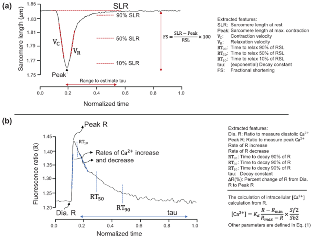
Machine learning model input features from (a) sarcomere length transient and (b) calcium transient. Additional features are the time to 10%, 50%, and 90% contraction of sarcomere as well as the time to 10%, 50%, and 90% to the peak value of R, not shown in the figure for brevity.

The ML input features calculated from sarcomere length curves are detailed in Fig. 1a and included initial and contracted sarcomere lengths (SL), contraction and relaxation velocities of SL, time for SL to decay by 10%, 50%, 90%, time for SL to peak by 10%, 50%, 90%, and fractional shortening. Fractional shortening is defined as the percentage of SL contraction from resting length to the peak contraction (Fig. 1a). The features of the calcium transient curve are shown in Fig. 1b and included systolic and diastolic [Ca²⁺], rate of [Ca²⁺] increase and decrease in the cell, time of [Ca²⁺] decay to 10%, 50%, and 90% of peak value, time of [Ca²⁺] to reach to 10%, 50%, and 90% to peak value, and percentage change of [Ca²⁺] from diastole to systole.

2.4. Classification models and evaluations metrics

The normal and impaired cells were classified using various ML classifiers, including (i) RF, (ii) SVM, (iii) KNN, (iv) DT, (v) LR, (vi) ADB, (vii) XGB, and (viii) MLP, and (ix) soft voting classifier. These classifiers were trained on data representing sarcomere length transient or calcium transient, with the aim of distinguishing between normal and impaired cells. The performance of each classifier was evaluated using the following measures: true positive (TP), representing actual and predicted true results; false positive (FP), representing actual true and predicted false results; false negative (FN), representing actual false and predicted true results; and true negative (TN), representing actual and predicted negative results. Subsequently, the following metric scores were developed using the TP, FP, FN, and TN measures:

1. The sensitivity metric was used to describe how often a classifier predicts correctly with correct data.

   $$Sensitivity=\text{TP}/(\text{TP}+\text{FN}).$$ (2)
2. The specificity metric was used to evaluate the model capability by estimating true negatives for each available category.

   $$Specificity=\text{TN}/(\text{TN}+\text{FP}).$$ (3)
3. The accuracy metric was used to describe the model performance by how correctly a classifier classifies samples from the total number of input samples.

   $$\mathit{\text{Accuracy}}=(\text{TP}+\text{TN})/\text{Total},\text{Total}=\text{TP}+\text{TN}+\text{FP}+\text{FN}.$$ (4)
4. The precision metric was used to describe the quality of the classifier to predict true positives among the total positive predictions.

   $$Precision=\text{TP}/(\text{TP}+\text{FP}).$$ (5)
5. The F1 score combines both sensitivity and precision and is considered to be the most comprehensive metric to describe a classifier.

   $$F1-score=\frac{2\times precision\times sensitivity}{precision+sensitivity}$$ (6)

6. Receiver operating characteristic (ROC) curves were plotted using sensitivity against 1- specificity and the area under the ROC curve (AUROC) score was used as an overall metric to evaluate each classifier’s ability in distinguishing positive and negative classes.

7. Confusion matrix summarized the number of true positives, false positives, true negatives, and false negatives in the form of a table.

   Details regarding the implementation of each ML classifier with its hyperparameters are defined in the following sections.

2.4.1. Random forest

Random forest (RF) is an ensemble ML method that constructs multiple decision trees, constituting a forest of trees, during the training stage. Each tree in the forest predicts a class label for every sample in the testing period. The predicted class labels from each tree are then combined using a majority voting technique to make the final decision for each test datum⁴¹. The class label that receives the most votes is considered the most suitable label for the test datum. This process is repeated for every datum in the collection. This approach increases the stability and accuracy of each tree and reduces variance by influencing the overfitting of the model. In order to optimize the performance of the RF classifier, several hyperparameters need to be tuned. Among these hyperparameters, n_estimators refers to the number of decision trees to be constructed in the RF model. The parameter min_samples_split specifies the minimum number of samples required to split an internal node in each decision tree. Similarly, the parameter min_samples_leaf specifies the minimum number of samples required to be present at a leaf node of each decision tree. Finally, the parameter max_depth refers to the maximum depth of each decision tree. In this work, we optimized the values of these hyperparameters within the range of 50-200, 2-5, 1–3, and 3-unlimited for n_estimators, min_samples_split, min_samples_leaf, and max_depth, respectively.

2.4.2. Support vector machine

The support vector machine (SVM) is a widely used machine learning model for classification problems in supervised learning. One of the key benefits of SVM is its capability to handle non-linear data and its reduced risk of overfitting⁴². To make predictions, the algorithm separates the data into two classes utilizing an optimal hyperplane chosen according to the maximum margin from the closest points. The algorithm finds two parallel hyperplanes that can separate the data and maximize their distance using a dual formulation with Lagrange’s multiplier. After training, the SVM classifier can be used to predict the class of new instances based on their position relative to the hyperplane. The SVM employed in this study utilized hyperparameters consisting of two regularization parameters denoted by C and $\gamma$, which respectively govern the level of regularization and the shape of the decision boundary, as well as the kernel type that is employed to transform the input data into a higher dimensional space. The values of these hyperparameters were chosen within the ranges of 100-1000 for C, 0.1-0.0001 for $\gamma$, and “rbf” or “sigmoid” for the kernel type.

2.4.3. K-nearest neighbors

The KNN algorithm is regarded as a simple method in ML in which a classification prediction is made by identifying the most similar samples within the training data⁴³. When a new test sample is presented to the classifier, the algorithm computes the distance between the new sample and all the training samples using a distance metric, such as Euclidean or Manhattan distance. The k number of neighbors is selected based on this distance and their class labels are used to predict the class label of the new sample. The effectiveness of this algorithm can be impacted by noisy or irrelevant features present in the data, as well as the choice of distance metric. The KNN algorithm is sensitive to the value of k, which is taken as a hyperparameter. An appropriate value for k can be estimated using $k=\sqrt{n}$ for a training set with a large number of samples⁴⁴; however, this choice is not considered to be an optimal value for a small data set. Here, we chose k (number of neighbors) and p (power parameter) within the range of 5 to 10 and 2 to 5 , respectively.

2.4.4. Decision tree

The DT algorithm is a well-known machine learning algorithm used for classification tasks. It employs a tree-like structure to classify data items based on their attributes⁴⁵. The tree typically comprises several levels of nodes, with the topmost node known as the parent or root node and the rest referred to as child nodes. The internal nodes in the tree represent the evaluation of features or input variables and consist of a minimum of one child node. The classification process branches to the appropriate child node based on the evaluation outcome, with this process continuing until a leaf (terminal node) is reached, which represents the final decision outcome⁴¹. To fine-tune the DT algorithm, we optimized hyperparameters including the criterion (either gini or entropy), max_depth (ranging from 1 to 5), and min_samples_leaf (ranging from 1 to 5).

2.4.5. Logistic regression

LR is a robust algorithm in supervised machine learning that extends the general regression modeling to predict the likelihood of a particular instance occurring⁴⁶. LR estimates the likelihood of a new observation belonging to a certain class, with its probability ranging from 0 to 1. In LR, observations with probabilities greater than 0.5 are classified as one class, while those with probabilities lower than 0.5 are classified as the other. If the categorical variable has more than two values, then logistic regression can be extended as multinomial logistic regression⁴⁷. To enhance the performance of the logistic regression (LR) classifier, we performed hyperparameter tuning by testing various combinations of penalty regularization (L1 and L2), a range of C regularization parameter values (0.1-10), and different optimization algorithms, such as liblinear and saga, used to minimize the cost function.

2.4.6. Adaptive Boosting

ADB is a widely-used algorithm in the boosting family of ensemble learning that generates a weak learner using the initial training data and adjusts the data distribution based on the previous weak learner’s performance for the next round of training⁴⁸. In the subsequent step, the samples with lower prediction accuracy receive more attention. These weak learners are combined into a strong learner with varying weights. The algorithm begins with an unweighted training sample and constructs a classifier, such as a classification tree, which produces class labels. If a training data point is classified incorrectly, the weight of that point is increased, or “boosted“. A second classifier is then constructed using the new, unequal weights, and this process is repeated. For hyperparameter tuning of AdaBoost, we explored the space of hyperparameters which included the choice of a base learner, the number of estimators varying within 50-1000, and the learning rate ranging from 0.1 to 1.

2.4.7. Extreme gradient boosting

The XGB model is based on a gradient-boosting decision tree (GBDT), which combines weak learning models to generate a collective strong model. The residual is used to improve the previous predictor by minimizing the loss function at each iteration of GBDT⁴⁹. The prediction is acquired by aggregating the output values of all the trees; nevertheless, overfitting may arise in trees and can be prevented by incorporating regularization penalties and manipulating the learning rate. The modification in the learning rate encompasses scaling down the weights of each tree by a small factor, which assists in regularizing the model and diminishing the effect of individual trees on the ultimate outcome. The performance of the XGBoost model was optimized by exploring the effects of various hyperparameters. Specifically, we varied the number of estimators (n_estimator) between 100 to 1000, the maximum depth of each tree (max_depth) between 3 to 10, and the learning rate between 0.01 to 1.

2.4.8. Multilayer perceptron

The MLP is a feedforward neural network that processes information in layers, with the input layer connected to the output layer via hidden layers. Each connection between neurons has a weight, and each layer of perceptrons has the same activation function, typically a sigmoid function for hidden layers. The output layer can have a sigmoid or linear function, depending on the application. During training, the MLP uses backpropagation that enables the MLP to adjust its weights by propagating errors from the output layer back to the input layer⁵⁰. The objective is to minimize the difference between the predicted and actual outputs. The performance of an MLP classifier depends on the training data, and training parameters such as learning rate, regularization parameters, activation function, and the number of hidden layers. In this work, the hyperparameters tuning of the MLP classifier involved varying the number of hidden layers from 1 to 3 with sizes ranging from 32 to 128, regularization parameter alpha from 0.0001 to 0.01, and using either a constant or adaptive learning rate with ReLU activation function.

2.4.9. Soft-voting classifier

We utilized a soft voting classifier to combine the individual classification models based on RF, LR, XGB, and MLP for sarcomere length transient, as well as RF, LR, KNN, and MLP for calcium transient features. These individual classifiers have demonstrated good performance in classification (AUC≥0.90) when trained individually. The soft voting classifier aggregates the predictions of these base classifiers by taking into account their respective probabilities. By combining the strengths of multiple classifiers, the voting-based classifier is expected to have better overall performance than any participant individual classifier. Additionally, the diversity of the individual classifiers could be beneficial for accurately predicting both positive and negative values, as some classifiers may perform well for normal cells and others may perform well for impaired cells.

2.5. ML training

To optimize the performance of ML classifiers, the grid search cross-validation method was employed. Initially, the complete dataset comprising normal and impaired cells was randomized, and the data was partitioned into ten sets of paired training and test data. Each training dataset was further partitioned such that 1/10 of the training data was reserved as a validation set for the purpose of tuning hyperparameters as shown in Fig. 2. Next, the hyperparameters of each model were tuned using a grid search over the hyperparameter space. The performance metrics, such as AUROC curve and F1-score, were used to evaluate the models on the validation set. The hyperparameters that yielded the highest AUROC score and F1-score on any validation set were selected for the final model training. Finally, the models were retrained using the chosen hyperparameters across all ten data partitions as depicted in Fig. 2, and the performance metrics were evaluated on the test data for each partition.

Fig. 2.

Machine learning classifier selection to classify normal and impaired cells.

2.6. Layer-wise relevance propagation

Layer-wise Relevance Propagation (LRP) is a promising analysis and interpretation method used to understand the contribution of individual features in a neural network-based model. LRP operates by backpropagating the prediction of the trained network and determining the relevance score of each input feature. More specifically, for a given network layer with neurons k and its preceding layer with neurons j, assuming we know the relevance score of k neurons as $R_k$, the relevance score of neurons j in the preceding layer can be calculated using the following equation:

$$R_j=\sum _k\frac{z_{jk}}{{\sum }_j{z}_{jk}}{R}_k$$ (7)

where $z_{jk}=a_j{w}_{jk}$ with $a_j$ representing the activation of neuron j and $w_{jk}$ representing the weights connecting neurons j and k. We chose LRP to evaluate the importance and relevance of each feature to classification following our pilot study indicating that MLP outperforms other individual classifiers on both sets of input features, namely sarcomere length transient and calcium transient. LRP was then applied to MLP to determine the relative contributions of input features toward the classification of impaired versus normal cells.

3. Results

3.1. Hyperparameter tuning analysis

The classifier models were trained using a grid search method to tune the hyperparameters, as explained in Section 2.5. Table 1 displays the tuned hyperparameters for all eight classifier models trained with sarcomere length and calcium transients and reveals that optimal hyperparameters for each model vary depending on the input features, and model performance may be highly sensitive to the choice of hyperparameters. For instance, the KNN model trained with sarcomere length transient performed best with k=5 and p=5, whereas the same model trained with calcium transient indicated k=9 and p=2 as optimal hyperparameters.

Table 1.

Best hyperparameters search using grid search cross-validation for random forest (RF), support vector machine (SVM), K-nearest neighbors (KNN), decision tree (DT), logistic regression (LR), adaptive boosting (ADB), extreme gradient boosting (XGB), and multilayer perceptron (MLP) trained for sarcomere length transient and calcium transient in classification problems.

ML classifiers	Hyperparameters		Sarcomere length transient	Calcium transient
RF	n_estimators		200	200
	min_samples_split		3	5
	min_samples_leaf		2	1
	max_depth		5	5
SVM	C:	Regularization	1000	100
	γ:	parameters	0.0001	0.01
		kernel	rbf	sigmoid
KNN	n_neighbors		5	9
	p		5	2
DT	criterion		gini	entropy
	max_depth		1	5
	min_samples_leaf		1	3
LR	C		5	3
	penalty		L1	L2
	solver		liblinear	liblinear
ADB	n_estimator		500	100
	learning_rate		1.0	0.1
XGB	n_estimator		100	100
	max_depth		7	5
	learning_rate		0.1	0.01
MLP	Number of hidden layers		1	1
	Size of hidden layers		256	256
	alpha		0.0001	0.0001
	learning_rate		constant	constant
	activation function		relu	relu

3.2. Performance evaluation of machine learning classifiers

The evaluation of the ML classifiers was conducted based on the analysis of the confusion matrices and ROC curves. Confusion matrices, depicting the number of correctly and incorrectly classified samples, were used to evaluate the performance of the classifiers. The ROC curve plots the true positive rate (sensitivity) against the false positive rate (1-specificity) at varying classification thresholds to assess the accuracy of the classifier predictions. Here, the results shown in Figures 3,6 and Table 2 relate to classifiers trained on sarcomere length transient. Results presented in Figures 4,7 and Table 3 relate to classifers trained on calcium transient. The F1-scores, sensitivity, specificity, precision, and accuracy were obtained from the confusion matrices of Figures 6 and 7 while the AUROC scores were obtained from Figures 3 and 4. These results are described in the following sections in detail. The comparison of the AUROC score and F1-score are displayed in Fig. 5a and b for both input features.

Fig. 3.

Receiver operating characteristics curves of eight individual classifiers as well as soft voting classifier consisting of random forest, logistic regression, extreme gradient boosting, and multilayer perceptron using sarcomere length transient as input features.

Fig. 6.

Confusion matrices of eight individual classifiers as well as soft voting classifier consisting of random forest, logistic regression, extreme gradient boosting, and multilayer perceptron using sarcomere length transient as input features.

Table 2.

Metric scores of eight individual classifiers as well as soft voting classifier consisting of random forest, logistic regression, extreme gradient boosting, and multilayer perceptron trained with sarcomere length transient features. The best-performing classifier is highlighted in red.

ML classifiers	Sensitivity	Specificity	Precision	Accuracy	F1-score
Random Forest	0.8679	0.8082	0.7667	0.8333	0.8142
Support vector machine	0.8824	0.80	0.75	0.8333	0.8108
K-nearest neighbors	0.8478	0.7375	0.65	0.7778	0.7358
Decision tree	0.8889	0.6869	0.5333	0.746	0.6667
Logistic regression	0.7966	0.806	0.7833	0.8016	0.7899
Adaptive boosting	0.7385	0.8033	0.80	0.7698	0.768
Extreme gradient boosting	0.8254	0.8730	0.8667	0.8492	0.8455
Multilayer perceptron	0.8644	0.8657	0.85	0.8651	0.8571
Soft voting	0.8909	0.8451	0.8167	0.8651	0.8522

Fig. 4.

Receiver operating characteristics curves of eight individual classifiers as well as soft voting classifier consisting of random forest, logistic regression, K-nearest neighbors, and multilayer perceptron using calcium transient as input features.

Fig. 7.

Confusion matrices of eight individual classifiers as well as soft voting classifier consisting of random forest, logistic regression, K-nearest neighbors, and multilayer perceptron using calcium transient as input features.

Table 3.

Metric scores of eight individual classifiers as well as soft voting classifier consisting of random forest, logistic regression, K-nearest neighbors, and multilayer perceptron trained with calcium transient features. The best-performing classifier is highlighted in red.

ML classifiers	Sensitivity	Specificity	Precision	Accuracy	F1-score
Random Forest	0.8519	0.8226	0.807	0.8362	0.8288
Support vector machine	0.8214	0.8167	0.807	0.819	0.8142
K-nearest neighbors	0.8182	0.8033	0.7895	0.8103	0.8036
Decision tree	0.7719	0.7797	0.7719	0.7759	0.7719
Logistic regression	0.8750	0.8667	0.8596	0.8707	0.8673
Adaptive boosting	0.7759	0.7931	0.7895	0.7845	0.7826
Extreme gradient boosting	0.7544	0.7627	0.7544	0.7586	0.7544
Multilayer perceptron	0.8596	0.8644	0.8596	0.8621	0.8596
Soft voting	0.8909	0.8689	0.8596	0.8793	0.8750

Fig. 5.

Comparison of AUROC and F1-scores for different classifiers trained with: (a) sarcomere length transient and (b) calcium transient. The best-performing classifiers are highlighted in red.

3.2.1. Assessment of sensitivity, specificity, accuracy, precision, and F1 score

To compare the trained classifiers, we performed calculations of various metrics, including sensitivity, specificity, precision, accuracy, and F1-score tabulated in Tables 2 and 3. These tables were obtained from Figures 6 and 7, which show confusion matrices for all classifiers trained using sarcomere length and calcium transient features, respectively. For classifiers trained on sarcomere length transient features (Table 2), the MLP classifier achieved the highest F1-score (0.8571) among individual classifiers. This score is indicative of a balance between the model’s sensitivity (0.8644), its ability to correctly identify normal cells, and its precision (0.85), which underscores the proportion of correctly identified normal cells out of all cases predicted as normal. These two measures collectively influence the F1-score, a harmonic mean of precision and sensitivity, which provides an overview of the model’s performance in terms of both false positives and false negatives. The MLP classifier’s specificity, an indication of its capacity to correctly identify impaired cases, was also notably high at 0.8657. This specificity, combined with the high sensitivity, resulted in an overall accuracy of 0.8651, demonstrating the model’s strong performance across both normal and impaired cases. When the soft voting classifier was trained on calcium transient features (Table 3), it achieved an F1-score of 0.8750, reflecting a similar balance between sensitivity (0.8909) and precision (0.8596). The model specificity of 0.8689 suggested a robust ability to correctly identify impaired cells, and the overall accuracy of 0.8793, suggested a strong performance across all classes.

3.2.2. Classifier performance based on AUROC scores

ROC curves were plotted for all classifiers trained using either sarcomere length transient or calcium transient features providing a comprehensive view of a classifier’s performance across varying decision thresholds, considering both sensitivity and specificity. The ROC curves with AUROC performance metric for the classifiers trained with sarcomere length or calcium transient features are illustrated in Figs. 3 and 4, respectively. The AUROC, a measure that considers the trade-off between sensitivity (ability to detect diseased cases) and specificity (ability to avoid falsely classifying healthy cases as diseased), was notably high for the soft voting classifier on both feature sets, indicating its excellent discriminative power across different decision thresholds. An AUROC score of 1.0 would indicate a perfect classifier, correctly distinguishing impaired and normal cases 100% of the time. Alternatively, an AUROC score of 0.5 indicates that the classifier has a 50% chance of misclassifying a given sample. When trained on sarcomere length transient features, the classifier achieved an AUROC score of 0.94. Similarly, while using calcium transient features, the classifier exhibited an AUROC score of 0.95. These high scores signify the classifier’s strong ability to differentiate between impaired and normal cases, irrespective of the decision threshold. Therefore, the soft voting classifier demonstrated excellent classification capability. It exhibited a high likelihood of correctly ranking a randomly selected impaired case higher than a randomly selected normal case.

3.3. Relevance scores of sarcomere length and calcium transients

The relevance scores obtained from LRP suggest that certain features have a higher relevance score than others, indicating their larger contribution towards the overall classification performance. Specifically, we found that time to 50% contraction of the sarcomere, the maximum contracted sarcomere length and time to 90% relaxation of the sarcomere showed the highest relevance scores, while time to 10% contraction of the sarcomere and relaxation time constant had the lowest relevance scores (Fig. 8a). For calcium transient data, time to 50% decay of R, rate of R decrease, and diastolic ratio exhibited the highest relevance score, while relaxation time constant tau and time to decay 90% of R had the lowest relevance score (Fig. 8b). The relevance scores for the normal cell samples did not significantly differ from the relevance scores obtained for the impaired cell samples. For brevity, they are not included here.

Fig. 8.

Relevance scores obtained from layer-wise relevance propagation of: (a) sarcomere length transient and (b) calcium transient. All features are defined in Fig. 1. Here V: velocity, SL: sarcomere length.

4. Discussion

4.1. Effect of input features on cell classification

In this study, we aimed to make use of ML algorithms to classify normal and impaired cardiomyocytes from sarcomere length transient data or calcium transient data. Our results demonstrated that the performance of each classifier can vary significantly depending on the input features used for training. For instance, the DT classifier indicated an AUROC of 0.66 when trained with sarcomere length transient features, while the same classifier trained with calcium transient features showed an AUROC of 0.82. In contrast, the high-performing soft voting classifier showed a similarly high AUROC when trained with either sarcomere length transient or calcium transient features. Overall, both sets of input features were able to provide a clear distinction between normal and impaired cells, with all AUROC values above 0.8, except for DT trained with sarcomere length transient. Our observations highlight the need for further exploration with regard to distinct datasets, and possible combinations of datasets, that could be used to improve the accuracy of such ML classification models. While classification models, such as the one presented here, hold the promise to enrich the metrics available to identify cells with impaired relaxation in an ex-vivo, controlled setting, exploration of the cellular metrics most pertinent to cell classification in vivo remains to be explored.

4.2. Performance comparison of different classifiers

The findings of this study demonstrate the importance of selecting appropriate classifiers for specific datasets based on the analysis of performance metrics reported in Fig. 5 and Tables 2–3.

Among the individual classifiers, MLP was found to be an excellent algorithm for the cell classification problem presented in this work. MLP showed the highest F1-score, accuracy, and AUROC scores out of all individual classifiers when using either sarcomere length transient or calcium transient features as input. MLP performance was followed closely by RF, LR, and XGB models trained with sarcomere length transient. Considering models trained on calcium transient features, RF, KNN, and LR classifiers approached the performance of MLP. In contrast, DT showed the lowest performance when considering all classifiers trained on either sarcomere length transient or calcium transient features, suggesting that DT is not an optimal choice for classifying normal and impaired cells with the present features.

The combination of four individual classifiers using soft voting outperformed the individual classifiers for sarcomere length transient as well as calcium transient features. The high performance of the MLP classifier was not compromised when combined with RF, LR, and XGB classifiers for sarcomere length transient or with RF, LR, and KNN classifiers for calcium transient features in the soft voting classifier. The soft voting classifier consistently outperformed the individual classifiers, regardless of the type of input features used.

Overall, our results indicate that the selection of an appropriate classifier for a specific dataset is crucial for achieving high classification accuracy.

4.3. Comparison with previous studies

Previous studies have utilized in-vitro cultured cells and calcium transient data to train ML classifiers for the classification of normal and diseased cells. Hwang et al. employed a SVM classifier and achieved an accuracy of 87%³³. Juhola et al. utilized a RF classifier to classify different diseases, including long QT syndrome and hypertrophic cardiomyopathy, based on abnormal calcium transients, achieving a maximum accuracy of 87.6%. In multi-classification scenarios, the RF classifier attained the highest accuracy of 78.6%, followed by SVM and KNN at 75.3% and 75.1%, respectively³⁴. In another study, Juhola et al. achieved an average accuracy of 80% by classifying calcium peaks into normal or abnormal categories³⁵. Despite the differences in methodology and data, our models, when viewed in light of these studies, show compelling performance. Our machine learning models, trained with sarcomere length transient and calcium transient data, yielded accuracy scores of 0.8651 and 0.8793, as well as an AUROC score of 0.94 and 0.95, respectively. Despite the different approaches and datasets, our results demonstrate comparable performance to those available in the literature.

4.4. Contribution of input features

The relevance scores obtained from LRP analysis for calcium transient features indicated high scores for all input features related to the relaxation of the sarcomere, suggesting a strong correlation between relaxation features of calcium transient. This finding was consistent with the comparatively high AUC values obtained for all classifiers trained with calcium transient, as compared to those trained with sarcomere length transient, shown in Figs. 3 and 4. However, none of the features provided an extremely low relevance score that would warrant their exclusion, and as a result, classification was not performed using a reduced set of input features. LRP was used to obtain relevance scores for all the input features in the sarcomere length transient and calcium transient datasets, revealing their contributions towards accurately classifying normal and impaired cardiomyocytes. We found that time to 50% contraction of the sarcomere showed the highest relevance scores for sarcomere length transient data, and, interestingly, time to 50% decay of [Ca²⁺] exhibited the highest relevance score for calcium transient data. Although some features had lower relevance scores, none were deemed insignificant enough to be discarded for classification purposes.

4.5. Implications and future directions

4.5.1. Identification of cardiomyocytes with impaired relaxation ex vivo and in vivo

Contraction-relaxation behavior of the sarcomere and intracellular Ca²⁺ transient are typically assessed ex vivo using contractility tests on isolated cardiomyocytes³⁹. These tests generate time-evolving data on intracellular [Ca²⁺] and sarcomere length, which can be used to identify and characterize contractility and relaxation impairments. However, the in-vivo measurement of Ca²⁺ and sarcomere dynamics remains challenging, despite the significant advances in imaging techniques. While multiphoton microscopy and genetically encoded calcium indicators were recently combined to record neuronal Ca²⁺ activity, such techniques are difficult to apply to a beating heart in the closed chest^51–53. Additionally, current cardiac imaging modalities and associated post-processing require further improvements to increase the fidelity of measuring myofiber length transient in vivo. Given these challenges, our presented approaches are limited to ex-vivo features, although they can be extended to in-vivo assessment once either the sarcomere length transient or Ca²⁺ transient cycle can be obtained in vivo. Additional considerations for the extension of our approach to in-vivo identification of cardiomyocytes with impaired relaxation are discussed in Limitations.

4.5.2. Predicting calcium transient from fiber kinematics

Quantification of the relaxation velocity of the sarcomere can be obtained from the sarcomere length transient data, which is calculated as the time for length to reduce by 50% from the peak value $(R{T}_{50}$: the relaxation half-time)⁵⁴. Relaxation velocity and other kinematics parameters (such as fractional shortening) are heavily influenced by Ca²⁺ transient^55,56. Given the strong calcium transient and sarcomere length transient relationship enabling the classification of cell status, a machine learning regression model^57,58 is expected to be able to predict calcium features (such as [Ca²⁺]) from sarcomere length data and relaxation velocity. To the best of our knowledge, the ability to predict Ca²⁺ transient from fiber kinematics data, using machine learning, remains unexplored while offering significant translational potential. The present study serves as a promising first step corroborating the possibility of using sarcomere length transient data to predict calcium kinetics which remains challenging to measure in vivo.

4.6. Limitations

Ex-vivo studies provide valuable insights into the classification of normal and impaired cardiomyocytes using sarcomere length transient and calcium transient. However, several limitations exist regarding their application to in-vivo settings. Primarily, the in-vivo condition involves intraventricular pressure load as well as electrophysiological activities that collectively drive and regulate cardiac motion. Therefore, these additional features need to be added to myofilament kinematics input estimated from medical imaging to enable ML classifiers to identify regions in the myocardium expressing impaired relaxation. Therefore, while the presented ML classification using ex-vivo data demonstrated the conceptual capability to identify the status of the cells based on their sarcomere length transient or calcium transient, additional considerations are needed to upgrade these classifiers for the in-vivo classification of cardiomyocytes using cardiac imaging inputs.

5. Conclusion

In this study, we aimed to demonstrate the ability of various ML models to classify cells with normal and impaired relaxation using sarcomere length transient or intracellular calcium transient data.

For this proof-of-concept study, we employed nine ML models, including RF, SVM, KNN, DT, LR, AdaBoost, XGBoost, MLP, and soft voting classifier to classify normal and impaired cells from sarcomere length and calcium transient features. Furthermore, each classifier was trained separately on sarcomere length transient or calcium transient features. Our findings suggest that the choice of input features and classifier are crucial for achieving high performance. We found that soft voting classifier and MLP consistently outperformed all other classifiers, regardless of the dataset used for training. Notably, the limited dataset used in this study still yielded reasonable accuracy, suggesting the potential for even higher accuracy with the inclusion of a greater number of samples in the training set. LRP analysis showed that relevance score for time to 50% contraction of the sarcomere was the highest for sarcomere length transient, while the highest relevance score for calcium transient input features was observed for time to 50% decay of R. Overall, our findings underscore the possibility of using ML classifiers to identify cardiomyocytes with impaired diastolic and systolic behaviors using common passive and contractile features obtained from the cells. Additionally, this work serves as an initial step towards the goal of integrating ML technology with physiological measurements and advanced cardiac strain imaging to enable the classification of cells directly from the in vivo data currently obtained from the beating heart in mice and humans.

Data availability

The data that support the findings of this study are available from the corresponding author, R.A., upon request.

References

- 1.Goldsborough E, Osuji N & Blaha MJ Assessment of cardiovascular disease risk: A 2022 update. Endocrinol. Metab. Clin 51, 483–509 (2022). [DOI] [PubMed] [Google Scholar]
- 2.Lopez AD, Mathers CD, Ezzati M, Jamison DT & Murray CJ Global and regional burden of disease and risk factors, 2001: systematic analysis of population health data. The lancet 367, 1747–1757 (2006). [DOI] [PubMed] [Google Scholar]
- 3.Del Buono MG, Buckley L & Abbate A Primary and secondary diastolic dysfunction in heart failure with preserved ejection fraction. The Am. journal cardiology 122, 1578–1587 (2018). [DOI] [PMC free article] [PubMed] [Google Scholar]
- 4.LeWinter MM & Meyer M Mechanisms of diastolic dysfunction in heart failure with a preserved ejection fraction: if it’s not one thing it’s another (2013). [DOI] [PMC free article] [PubMed]
- 5.Owan TE et al. Trends in prevalence and outcome of heart failure with preserved ejection fraction. New Engl. J. Medicine 355, 251–259 (2006). [DOI] [PubMed] [Google Scholar]
- 6.Tribouilloy C. et al. Prognosis of heart failure with preserved ejection fraction: a 5 year prospective population-based study. Eur. heart journal 29, 339–347 (2008). [DOI] [PubMed] [Google Scholar]
- 7.Zile MR & Brutsaert DL New concepts in diastolic dysfunction and diastolic heart failure: Part i: diagnosis, prognosis, and measurements of diastolic function. Circulation 105, 1387–1393 (2002). [DOI] [PubMed] [Google Scholar]
- 8.Aurigemma GP & Gaasch WH Diastolic heart failure. New Engl. J. Medicine 351, 1097–1105 (2004). [DOI] [PubMed] [Google Scholar]
- 9.Gaasch WH & Zile MR Left ventricular diastolic dysfunction and diastolic heart failure. Annu. Rev. Med 55, 373–394 (2004). [DOI] [PubMed] [Google Scholar]
- 10.Zile MR, Baicu CF & Gaasch WH Diastolic heart failure—abnormalities in active relaxation and passive stiffness of the left ventricle. New Engl. J. Medicine 350, 1953–1959 (2004). [DOI] [PubMed] [Google Scholar]
- 11.Katz AM & Lorell BH Regulation of cardiac contraction and relaxation. Circulation 102, Iv–69 (2000). [DOI] [PubMed] [Google Scholar]
- 12.Calaghan S & White E The role of calcium in the response of cardiac muscle to stretch. Prog. biophysics molecular biology 71, 59–90 (1999). [DOI] [PubMed] [Google Scholar]
- 13.Asp ML, Martindale JJ, Heinis FI, Wang W & Metzger JM Calcium mishandling in diastolic dysfunction: mechanisms and potential therapies. Biochimica et Biophys. Acta (BBA)-Molecular Cell Res. 1833, 895–900 (2013). [DOI] [PMC free article] [PubMed] [Google Scholar]
- 14.Bers D. Excitation-contraction coupling and cardiac contractile force, vol. 237 (Springer Science & Business Media, 2001). [Google Scholar]
- 15.Niederer S, Hunter P & Smith N A quantitative analysis of cardiac myocyte relaxation: a simulation study. Biophys. journal 90, 1697–1722 (2006). [DOI] [PMC free article] [PubMed] [Google Scholar]
- 16.Bers DM Cardiac excitation–contraction coupling. Nature 415, 198–205 (2002). [DOI] [PubMed] [Google Scholar]
- 17.Stern MD Theory of excitation-contraction coupling in cardiac muscle. Biophys. journal 63, 497–517 (1992). [DOI] [PMC free article] [PubMed] [Google Scholar]
- 18.Kumar M, Haghighi K, Kranias EG & Sadayappan S Phosphorylation of cardiac myosin–binding protein-c contributes to calcium homeostasis. J. Biol. Chem 295, 11275–11291 (2020). [DOI] [PMC free article] [PubMed] [Google Scholar]
- 19.Keshavarzian M. et al. Left ventricular free wall adaptations in heart failure with preserved ejection fraction: Insights from a murine model. Circulation 144, A14317–A14317 (2021). [Google Scholar]
- 20.Neelakantan S. et al. Abstract p3022: Multiscale characterization of left ventricular diastolic dysfunction in diabetic and cardiac myosin binding protein-c phospho-ablated murine models. Circ. Res 131, AP3022–AP3022 (2022). [Google Scholar]
- 21.Neelakantan S. et al. Multiscale characterization of left ventricle active behavior in the mouse. Acta Biomater. (2023). [DOI] [PMC free article] [PubMed] [Google Scholar]
- 22.Mandinov L, Eberli FR, Seiler C & Hess OM Diastolic heart failure. Cardiovasc. research 45, 813–825 (2000). [DOI] [PubMed] [Google Scholar]
- 23.Silbiger JJ Pathophysiology and echocardiographic diagnosis of left ventricular diastolic dysfunction. J. Am. Soc. Echocardiogr 32, 216–232 (2019). [DOI] [PubMed] [Google Scholar]
- 24.Fernandez-Perez G, Duarte R, De la Calle MC, Calatayud J & González JS Analysis of left ventricular diastolic function using magnetic resonance imaging. ιa(English Ed. 54, 295–305 (2012). [DOI] [PubMed] [Google Scholar]
- 25.Avazmohammadi R. et al. A contemporary look at biomechanical models of myocardium. Annu. review biomedical engineering 21, 417–442 (2019). [DOI] [PMC free article] [PubMed] [Google Scholar]
- 26.Hamdani N. et al. Sarcomeric dysfunction in heart failure. Cardiovasc. research 77, 649–658 (2008). [DOI] [PubMed] [Google Scholar]
- 27.Davies C. et al. Reduced contraction and altered frequency response of isolated ventricular myocytes from patients with heart failure. Circulation 92, 2540–2549 (1995). [DOI] [PubMed] [Google Scholar]
- 28.Williams B. et al. Prediction of human induced pluripotent stem cell cardiac differentiation outcome by multifactorial process modeling. Front. bioengineering biotechnology 8, 851 (2020). [DOI] [PMC free article] [PubMed] [Google Scholar]
- 29.Orita K, Sawada K, Koyama R & Ikegaya Y Deep learning-based quality control of cultured human-induced pluripotent stem cell-derived cardiomyocytes. J. pharmacological sciences 140, 313–316 (2019). [DOI] [PubMed] [Google Scholar]
- 30.Orita K, Sawada K, Matsumoto N & Ikegaya Y Machine-learning-based quality control of contractility of cultured human-induced pluripotent stem-cell-derived cardiomyocytes. Biochem. biophysical research communications 526, 751–755 (2020). [DOI] [PubMed] [Google Scholar]
- 31.Lee EK et al. Machine learning of human pluripotent stem cell-derived engineered cardiac tissue contractility for automated drug classification. Stem Cell Reports 9, 1560–1572 (2017). [DOI] [PMC free article] [PubMed] [Google Scholar]
- 32.Zhu R, Millrod MA, Zambidis ET & Tung L Variability of action potentials within and among cardiac cell clusters derived from human embryonic stem cells. Sci. reports 6, 1–12 (2016). [DOI] [PMC free article] [PubMed] [Google Scholar]
- 33.Hwang H, Liu R, Maxwell JT, Yang J & Xu C Machine learning identifies abnormal ca 2+ transients in human induced pluripotent stem cell-derived cardiomyocytes. Sci. reports 10, 16977 (2020). [DOI] [PMC free article] [PubMed] [Google Scholar]
- 34.Juhola M, Joutsijoki H, Penttinen K & Aalto-Setälä K Detection of genetic cardiac diseases by ca2+ transient profiles using machine learning methods. Sci. reports 8, 9355 (2018). [DOI] [PMC free article] [PubMed] [Google Scholar]
- 35.Juhola M. et al. Signal analysis and classification methods for the calcium transient data of stem cell-derived cardiomyocytes. Comput. Biol. Medicine 61, 1–7 (2015). [DOI] [PubMed] [Google Scholar]
- 36.Peters MF, Lamore SD, Guo L, Scott CW & Kolaja KL Human stem cell-derived cardiomyocytes in cellular impedance assays: bringing cardiotoxicity screening to the front line. Cardiovasc. Toxicol 15, 127–139 (2015). [DOI] [PubMed] [Google Scholar]
- 37.Cheng Y. et al. Impaired contractile function due to decreased cardiac myosin binding protein c content in the sarcomere. Am. J. Physiol. Circ. Physiol 305, H52–H65 (2013). [DOI] [PMC free article] [PubMed] [Google Scholar]
- 38.Haghighi K. et al. Human g109e-inhibitor-1 impairs cardiac function and promotes arrhythmias. J. molecular cellular cardiology 89, 349–359 (2015). [DOI] [PMC free article] [PubMed] [Google Scholar]
- 39.Bidwell PA, Haghighi K & Kranias EG The antiapoptotic protein hax-1 mediates half of phospholamban’s inhibitory activity on calcium cycling and contractility in the heart. J. Biol. Chem 293, 359–367 (2018). [DOI] [PMC free article] [PubMed] [Google Scholar]
- 40.Grynkiewicz G, Poenie M & Tsien RY A new generation of ca2+ indicators with greatly improved fluorescence properties. J. biological chemistry 260, 3440–3450 (1985). [PubMed] [Google Scholar]
- 41.Quinlan JR Induction of decision trees. Mach. learning 1, 81–106 (1986). [Google Scholar]
- 42.Hua J, Xiong Z, Lowey J, Suh E & Dougherty ER Optimal number of features as a function of sample size for various classification rules. Bioinformatics 21, 1509–1515 (2005). [DOI] [PubMed] [Google Scholar]
- 43.Zhang S, Cheng D, Deng Z, Zong M & Deng X A novel knn algorithm with data-driven k parameter computation. Pattern Recognit. Lett 109, 44–54 (2018). [Google Scholar]
- 44.Hassanat AB, Abbadi MA, Altarawneh GA & Alhasanat AA Solving the problem of the k parameter in the knn classifier using an ensemble learning approach. arXiv preprint arXiv:1409.0919 (2014). [Google Scholar]
- 45.Uddin S. Factors related the job satisfaction among migrant nurses in qatar. South East Asia Nurs. Res 1, 1 (2019). [Google Scholar]
- 46.Hosmer DW Jr, Lemeshow S & Sturdivant RX Applied logistic regression, vol. 398 (John Wiley & Sons, 2013). [Google Scholar]
- 47.Dreiseitl S & Ohno-Machado L Logistic regression and artificial neural network classification models: a methodology review. J. biomedical informatics 35, 352–359 (2002). [DOI] [PubMed] [Google Scholar]
- 48.Hastie T, Rosset S, Zhu J & Zou H Multi-class adaboost. Stat. its Interface 2, 349–360 (2009). [Google Scholar]
- 49.Dong W, Huang Y, Lehane B & Ma G Xgboost algorithm-based prediction of concrete electrical resistivity for structural health monitoring. Autom. Constr 114, 103155 (2020). [Google Scholar]
- 50.Du K-L, Swamy M, Du K-L & Swamy M Fundamentals of machine learning. Neural Networks Stat. Learn 15–65 (2014). [Google Scholar]
- 51.Pologruto TA, Yasuda R & Svoboda K Monitoring neural activity and [ca2+] with genetically encoded ca2+ indicators. J. Neurosci 24, 9572–9579 (2004). [DOI] [PMC free article] [PubMed] [Google Scholar]
- 52.Chen T-W et al. Ultrasensitive fluorescent proteins for imaging neuronal activity. Nature 499, 295–300 (2013). [DOI] [PMC free article] [PubMed] [Google Scholar]
- 53.Prevedel R. et al. Fast volumetric calcium imaging across multiple cortical layers using sculpted light. Nat. methods 13, 1021–1028 (2016). [DOI] [PMC free article] [PubMed] [Google Scholar]
- 54.Janssen PM, Stull LB & Marbán E Myofilament properties comprise the rate-limiting step for cardiac relaxation at body temperature in the rat. Am. J. Physiol. Circ. Physiol 282, H499–H507 (2002). [DOI] [PubMed] [Google Scholar]
- 55.McIvoR ME, Orchard CH & Lakatta E Dissociation of changes in apparent myofibrillar ca2+ sensitivity and twitch relaxation induced by adrenergic and cholinergic stimulation in isolated ferret cardiac muscle. The J. general physiology 92, 509–529 (1988). [DOI] [PMC free article] [PubMed] [Google Scholar]
- 56.Backx PH, Gao W-D, Azan-Backx MD & Marban E The relationship between contractile force and intracellular [ca2+] in intact rat cardiac trabeculae. The J. general physiology 105, 1–19 (1995). [DOI] [PMC free article] [PubMed] [Google Scholar]
- 57.Babaei H. et al. A machine learning model to estimate myocardial stiffness from edpvr. Sci. Reports 12, 5433 (2022). [DOI] [PMC free article] [PubMed] [Google Scholar]
- 58.Mehdi RR et al. Comparison of three machine learning methods to estimate myocardial stiffness. .
Associated Data
This section collects any data citations, data availability statements, or supplementary materials included in this article.
Data Availability Statement