Normalization strategies for cDNA microarrays

Abstract

Multiple Arabidopsis thaliana clones from an experimental series of cDNA microarrays are evaluated in order to identify essential sources of noise in the spotting and hybridization process. Theoretical and experimental strategies for an improved quantitative evaluation of cDNA microarrays are proposed and tested on a series of differently diluted control clones. Several sources of noise are identified from the data. Systematic and stochastic fluctuations in the spotting process are reduced by control spots and statistical techniques. The reliability of slide to slide comparison is critically assessed within the statistical framework of pattern matching and classification.

INTRODUCTION

Large areas of medical research and biotechnological development will be transformed by the evolution of high throughput techniques (1–3). Miniaturization and automatization enables the concurrent performance of many thousands or even millions of small-scale experiments on oligonucleotide chips (4,5) or spotted microarrays (6–8). Manufacturing processes and labeling techniques will lead to different performances (9,10) and detection ranges (11), but questions of statistical significance (12,13) and quality control (T.Beissbarth, K.Fellenberg, B.Brors, A.Arribas-Prat, M.J.Boer, V.N.Hauser, M.Scheideler, D.J.Hoheisel, G.Schuetz, A.Poustka and M.Vingron, submitted for publication; 14) are quite similar for the different technologies.

Down-scaling of an experiment makes it generally sensitive to external and internal fluctuations (7). Since reliability of interaction patterns extracted from array data is essential for their interpretation (15,16), a reduction in these fluctuations by proper averaging and normalization procedures is of great practical interest (17). We will address this issue in the context of cDNA microarrays, spotted on glass slides and hybridized with a radioactively labeled probe.

According to the experimental steps listed in Materials and Methods we will now give a list of the major sources of fluctuations to be expected in this type of microarray experiment. The list addresses fluctuations in probe, target and array preparation, in the hybridization process, background and overshining effects and effects resulting from image processing.

• mRNA preparation: depending on tissue and sensitivity to RNA degradation probes may look very different from sample to sample.

• Transcription: reverse transcription to cDNA will result in DNA species of varying lengths.

• Labeling: radioactive labeling may fluctuate randomly and systematically depending on nucleotide composition.

• Amplification: clones are subject to PCR amplification, which is difficult to quantify and may fail completely.

• Systematic variations in pin geometry: pins have different characteristics and surface properties and therefore transport different amounts of target cDNA.

• Random fluctuations in target volume: the amount of transported target fluctuates stochastically even for the same pin.

• Target fixation: the fraction of target cDNA that is chemically linked to the slide surface from the droplet is unknown.

• Hybridization parameters: efficiency of the hybridization reaction is influenced by a number of experimental parameters, notably temperature, time, buffering conditions and the overall amount of probe molecules used for hybridization.

• Slide inhomogeneities: for different reasons the probe may be distributed unequally over the slide or the hybridization reaction may perform differently in different parts of the slide.

• Non-specific hybridization: a typical source of error that cannot be completely excluded.

• Non-specific background and overshining: non-specific radiation and signals from neighboring spots.

• Image analysis: non-linear transmission characteristics and saturation effects and variations in spot shape.

Different types of experiments are required for assessing different types of fluctuations. If possible, sources of noise should be selectively excluded allowing for a precise estimation of their influence. In this work we exclude variations in probe preparation by focusing on the normalization and classification of Arabidopsis control clones. Even within this simplified setting analysis remains complex: the signal collected from several different pins will include superimposed fluctuations, e.g. from random fluctuations in target volume, slide inhomogeneities and overshining effects. In the following, systematic and random fluctuations inherent to spotting and hybridization are estimated directly from the data; a substantial part of the systematic error can be removed by a refined normalization procedure.

MATERIALS AND METHODS

Array preparation

A complex probe from several mouse tissues was purified and reverse transcribed with radioactively labeled cDNA. Arabidopsis thaliana cDNA (GenBank accession nos AF104328 and U29785) was spiked in a fixed amount for normalization purposes (18). Clones were amplified by PCR reaction, 5′-amino-modified for attachment to glass slides, and purified (19). Prior to spotting, glass slides were cleaned and derivatized for covalent attachment of cDNA. A 384 pin gridding head (X5251; Genetix, Christchurch, UK) was used for spotting a grid of 384 blocks, each containing 36 spots. All clones were spotted twice within a block (double spotting).

Details of the spotting pattern of library and control clones are explained in Figure 1. Altogether nine slides with an identical spotting pattern were produced.

Figure 1.

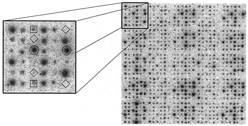
Segment from a 96 × 144 spot image of a cDNA microarray. The enlarged area (left) shows the spotting pattern (6 × 6 spots) produced by a single pin. Besides the different mouse clones (two spots each) the pattern contains four empty or background spots (diamonds), two spots from the constant Arabidopsis control (circles) and two spots belonging to the Arabidopsis dilution control series (squares). The dilution series consists of six steps, each corresponding to a 2-fold dilution. The gray levels in both graphics are presented on a logarithmic scale in order to give a better impression of the fuzzy boundaries of individual spots.

The radioactively labeled probe was hybridized on the cDNA array for 10 h at 42°C. For details on spotting technique and hybridization procedures see Eickhoff et al. (20).

Scanning and image processing

Arrays were exposed for 16 h to a Fuji BAS-SR 2025 intensifying screen (Raytest, Germany) and scanned at 25 µm resolution with a Fuji BAS 5000 phosphorimager (Raytest). The image was converted into a table of signal intensities using proprietary software.

Data processing

Intensity data were ordered in a table, each column corresponding to a slide and each row to a spot on the slide. The following normalization procedures were tested for their efficiency:

• no normalization, averaging over k slides;

• normalization by average intensity of control spots (slide-wise normalization) and averaging over k slides;

• division by the intensity of the two constant spots and averaging over k slides (pin-wise normalization);

• slide-wise normalization of the diluted and constant signals, averaging of the dilution and control signals over several slides, then quotient formation (average pin-wise normalization).

RESULTS

Non-specific background and overshining

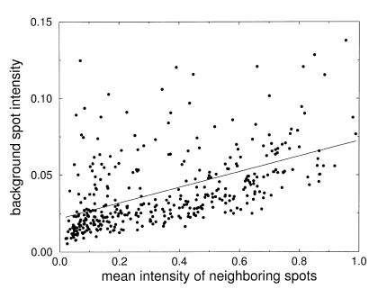
The level of background noise and the influence of neighboring signal intensities is illustrated in Figure 2. The intensity of background spots is plotted versus the average signal intensity of the four next neighbor spots.

Figure 2.

Intensity measured on background spots versus the mean intensity of the four neighboring spots. The slope of the linear interpolation is 0.051 with an axis intercept at 0.021. The corresponding correlation coefficient is C = 0.48.

The y-axis intercept of the linear regression gives an estimation of the non-specific background. The small background intensity indicates that there are only weak overshining effects for the 6 × 6 spotting pattern. The regression can be used for correction of the systematic part of these errors. The radius used to quantify spots was varied systematically: for the given spotting density only weak changes are observed if the scanning radius is kept in a reasonable range of about half the spotting distance (data not shown). The magnitude of the background and overshining effects is substantially smaller than fluctuations induced by spotting variabilities quantified below.

Assessment of spotting variabilities

In order to facilitate interpretation of the experimental data we neglect all non-linearities from image processing and assume that hybridization reactions reach mass action equilibrium. Due to the fact that different spots of a dilution series compete for the same probe the amount of probe bound in each spot is proportional to the amount of target cDNA present in the spot. The observed signal intensity then reflects the amount of spotted cDNA. Fluctuations in spot size and in the hybridization process can now be inferred from fluctuations in the signal gained from control spots. Scatter plots for typical experiments are presented in Figure 3 and give insight into the magnitude of fluctuations and correlations between double spotted signals.

Figure 3.

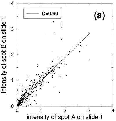
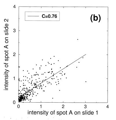
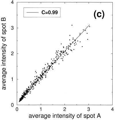
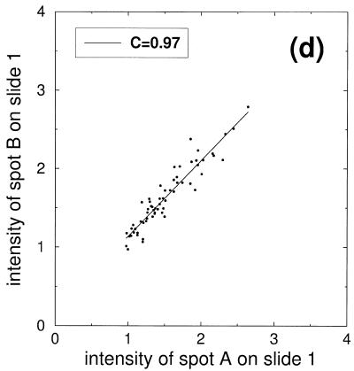
Scatter plots of the signal intensities obtained from a six step dilution series. (a) Points represent double spotted pairs from the same block of one slide. (b) Comparison of signal intensities from two different slides. (c) Comparison of signal intensities from nine slides after slide-wise normalization and averaging over the nine slides. (d) Subset of signal intensities from (c) corresponding to the second dilution level.

In Figure 3a signal intensities of the dilution series are shown. The 384 points represent double spotted pairs from the same block of one slide. Ideally the spots would form a straight line along the diagonal. Deviations from this ideal behavior essentially reflect random fluctuations in target volume (item 6 listed in the Introduction). Points are increasingly dense close to the origin owing to the construction of the dilution series: dilution is stepwise increased by a factor of two, resulting in an exponentially growing number of points in the region of low signal intensities. The correlation value of C = 0.90 gives an impression of the signal reproducibility within one block.

In Figure 3b intensity values of two slides are compared. The correlation is substantially smaller (C = 0.76) and the slope of 0.6 is significantly different from 1. The smaller correlation value indicates that additional sources of noise complicate the comparison of different slides. According to our reasoning above, the main sources of additional noise will be inhomogeneities in hybridization (items 8 and 9) as well as non-linear transmission and saturation effects in scanning and image processing (item 12). The fact that the cumulative intensity of all spots of the dilution series should be the same in all nine slides implies a simple normalization procedure: divide the signal intensity of each spot by the average intensity of all control spots on the slide. This intuitive normalization procedure will be referred to as ‘slide-wise normalization’. Applying slide-wise normalization to the example given in Figure 3b would result in a corrected slope close to 1. The values from different slides are now directly comparable, which is an obvious advantage of this normalization procedure.

Due to the stochastic character of the above-mentioned fluctuations, averaging is a sensible method to reduce the noise level. We demonstrate this by normalizing nine slides as described above and plotting the averaged normalized intensities (Fig. 3c). Scattering of the signal is considerably reduced, as reflected in the substantially higher correlation coefficient of C = 0.99. Despite the small deviations of the averaged signal from the diagonal, the six classes of the dilution series cannot be distinguished in the scatter plot in Figure 3c. This hints at the presence of another source of noise not reduced by this averaging procedure.

This variability stems from systematic variations in pin geometry, as clearly shown in Figure 3d. Here, only the points belonging to the second dilution level are plotted. If only stochastic sources of noise were present in the signal, a narrow circular distribution would be expected. In contrast, a correlation coefficient of C = 0.97 and a wide signal distribution indicate correlated variations in the signal that are present despite averaging over different slides. On the other hand, the strong correlations can be exploited for correction of the systematic deviations induced by different pin characteristics.

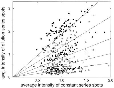
Figure 4 illustrates how the presence of a constant control signal can help to distinguish the different classes of the dilution series. The intensity of the averaged diluted control signal is plotted versus the intensity of the averaged constant control signal. Each dilution level is represented by 64 spots corresponding to 64 different pins (see Materials and Methods). If only the dilution signal is known the different classes will strongly overlap, as seen from projecting the points to the y-axis. In two dimensions, however, the six classes are reasonably well separated. Basically this is due to the fact that the reference signal helps to decide whether an observed strong signal intensity is due to high concentration in the target clone or rather a consequence of systematically excessive volume spotted by the corresponding pin. The most direct way to achieve normalization by the constant control signal is by calculating the ratio of the dilution signal and the constant control signal. In geometrical terms this corresponds to a projection of the data point along a ray from the origin onto the vertical axis. In the next section we investigate how suitable ways of averaging and normalization improve the separability of the dilution classes.

Figure 4.

Intensity of diluted control signal versus intensity of the constant control signal. Values are obtained by averaging over eight slides after normalization by slide average. The six different dilution classes are marked by six different symbols. Classes are separable to a fair degree in two dimensions, owing to correlations between the constant and diluted signals. Class boundaries as defined by the nearest mean classifier are indicated by lines

Classification of the dilution levels

Separation of the dilution levels based on signal strengths can be regarded as a classification task: given a randomly chosen position on the slide, infer the correct dilution class from the signal intensity observed at that point. Classification is perfect when all spots are assigned to the correct class. Of more practical importance than reassignment is prediction of signal intensity patterns of unknown class. This problem is comparable to the task of inferring an mRNA level from the signal intensity observed in a spot, where the probe rather than the target dilution is of interest. Classification and prediction are done with a nearest mean classifier (21). This classifier is represented by a number of center vectors, each vector defined as the center of one class. Any pattern classified by this method is associated with the class defined by the closest center. Two issues will be investigated:

• improvement of classification and prediction performance by averaging multiple experiments;

• improvement of classification and prediction performance by suitable normalization.

Improvement by averaging is assessed by dividing a set of eight slides into training and test sets of varying size. In four steps an increasing number of slides (k = 1, 2, 4 or 8) is used to infer the dilution class in a given position of the slide. For k = 1 the classification task is to recover the correct dilution class of a given spot using the nearest mean classifier trained on the same slide. The prediction task is to predict the correct dilution class of a given spot using the nearest mean classifier trained on a different slide. The quality of classification is measured by the percentage of correct assignments. For k = 2 or 4 (averaging over two or four slides) the whole procedure remains the same with the only difference that the classifier is now constructed by averaging signals from two or four slides and the prediction is done for two or four other slides. For eight slides only the classification task can be performed. The results for the four normalization procedures described in Materials and Methods are presented in Table 1. As seen from the first two rows, classification is little improved by slide-wise normalization. However, prediction of the test set is considerably better for the normalized data. The reason for this lies in the reduced signal variability in the normalized data. Averaging reduces random fluctuations and makes both the task of classification and that of prediction easier. Substantial improvement is possible by including the constant control spots in the normalization and thereby applying systematic corrections to variations in pin geometry.

Table 1. Percentage of correct classification and prediction for the nearest mean classifier using different normalization strategies.

Normalization	Average of
	One slide		Two slides		Four slides		Eight slides
	Training	Test	Training	Test	Training	Test	Training
(A) None	50	32	53	30	60	57	62
(B) Slide-wise	50	49	54	52	61	60	63
(C) Pin-wise	62	55	64	59	68	65	71
(D) Average pin-wise	63	58	70	69	75	74	78

The classifier is constructed by calculating centers of six classes from a set of training data. Then it is applied to reclassification of the same data (training) and to prediction of classes for data not in the training set (test). Increasingly large sets of data are averaged from the left column to the right column. Different normalization procedures explained in the text are applied in each line.

DISCUSSION

The evaluation performed for multi-spotted A.thaliana control clones allowed the identification of essential sources of noise resulting from the spotting and hybridization processes. Systematic signal fluctuations in target transmission during the spotting process can be reduced by monitoring control spots. Stochastic fluctuations can be reduced by averaging intensity values for the same target clone over multiple slides after suitable normalization.

More generally, normalization enables the combination of multiple measurements performed on different slides to an intensity vector. Any type of classification tool, like refined statistical indicators or neural networks, can be used to classify these vectors. A direct application of this strategy is demonstrated by the reduction in stochastic signal fluctuations in diluted control clones, leading to improved reclassifaction of the dilution classes. Since the correct classification is known in advance, an assessment of performance is possible (see Table 1). This allows judgement of the number of slides necessary for a desired signal resolution.

Comparing the four normalization schemes proposed, for our experiment the average pin-wise strategy (D) seems most appropriate. Training and test performance are persistently higher than in all other procedures. An explanation for this fact is given by the following consideration. By first calculating an average over several slides and then calculating the ratio of the averaged quantities, this strategy tends to avoid a strongly fluctuating denominator. This makes strategy (D) superior to strategy (C), where first the ratio of individual quantities is calculated and than an average is taken. Of course, the optimal strategy will depend on the relative amount of noise contributed by different sources and will very much depend on the array and labeling technique employed.

We envisage that the inclusion of control clones in every spotted array and spiking of these clones into the hybridization solution could be the initial step towards an enhanced comparability of microarray data, irrespective of where the array is produced. Normalization may be less important for the two-color labeling strategy, since ratios should be independent of the actual spot size. Generally, the comparison of different experiments (slides) will require some kind of normalization: either explicit by a defined set of normalization clones or implicit by a reference probe. The unavoidable use of a reference probe in the two-color labeling strategy may be a disadvantage if results from different laboratories are to be compared.

Although our considerations have concentrated on cDNA arrays using glass slides and radioactively marked probes, the principal sources of systematic and stochastic signal variability are expected to be similar in other microarray technologies involving spotting techniques. A proper normalization of array data will be a prerequisite to successfully meet future challenges like identification of SNPs, identification of expression profiles and reverse engineering of regulatory genetic networks.

REFERENCES

- 1.Gerhold D., Rushmore,T. and Caskey,C.T. (1999) Trends Biochem. Sci., 24, 168–173. [DOI] [PubMed] [Google Scholar]
- 2.Editorial (1999) Nature Genet., 21 (suppl.), 1. [Google Scholar]
- 3.Wen X., Fuhrmann,S., Michaelis,S.G., Carr,B.D., Smith,S., Barker,L.J. and Somogyi,R. (1998) Proc. Natl Acad. Sci. USA, 95, 334–339. [DOI] [PMC free article] [PubMed] [Google Scholar]
- 4.Lockhardt D.J., Dong,H., Byrne,M.C., Follettie,M.T., Gallo,M.V., Chee,M.S., Mittmann,M., Wang,C., Kobayashi,M., Horton,H. and Brown,E.L. (1996) Nature Biotechnol., 14, 1675–1689. [DOI] [PubMed] [Google Scholar]
- 5.Zhu H., Cong,J.-P., Mamtora,G., Gingeras,T. and Shenk,T. (1998) Proc. Natl Acad. Sci. USA, 95, 14470–14475. [DOI] [PMC free article] [PubMed] [Google Scholar]
- 6.Lennon G.C. and Lehrach,H. (1991) Trends Genet., 7, 314–317. [DOI] [PubMed] [Google Scholar]
- 7.Pietu G., Alibert,O., Guichard,V., Lamy,B., Bois,F., Leroy,E., Mariage-Samson,R., Houlgatte,R., Soularue,P. and Auffray,C. (1996) Genome Res., 6, 492–503. [DOI] [PubMed] [Google Scholar]
- 8.DeRisi J.L., Iyer,V.R. and Brown,P.O. (1997) Science, 278, 680–686. [DOI] [PubMed] [Google Scholar]
- 9.Granjeaud S., Bertucci,F. and Jordan,B.R. (1999) Bioessays, 21, 781–790. [DOI] [PubMed] [Google Scholar]
- 10.Richmond C.S., Glasner,J.D., Mau,R., Jin,H. and Blattner,F.R. (1999) Nucleic Acids Res., 27, 3821–3835. [DOI] [PMC free article] [PubMed] [Google Scholar]
- 11.Duggan D.J., Bittner,M., Chen,Y., Metzner,P. and Trent,J.M. (1999) Nature Genet., 21 (suppl.), 10–14. [DOI] [PubMed] [Google Scholar]
- 12.Audic A. and Claverie,J.-M. (1997) Genome Res., 7, 986–995. [DOI] [PubMed] [Google Scholar]
- 13.Claverie J.-M. (1999) Hum. Mol. Genet., 10, 1821–1832. [DOI] [PubMed] [Google Scholar]
- 14.Vingron M. and Hoheisel,J. (1999) J. Mol. Med., 77, 3–7. [DOI] [PubMed] [Google Scholar]
- 15.Brazma A., Jonassen,I., Vilo,J. and Ukkonen,E. (1998) Genome Res., 8, 1202–1215. [DOI] [PMC free article] [PubMed] [Google Scholar]
- 16.Somogyi R. and Sniegosky,C.A. (1996) Complexity., 1, 45–63. [Google Scholar]
- 17.Loftus K.S., Chen,Y., Gooden,G., Ryan,J.F., Birznieks,G., Hillard,M., Baxevanis,D.A., Bittner,M., Meltzer,P., Trent,J. and Pavan,W. (1999) Proc. Natl Acad. Sci. USA, 96, 9277–9280. [DOI] [PMC free article] [PubMed] [Google Scholar]
- 18.Eickhoff B., Korn,B., Schick,M., Prouska,A. and van der Bosch,J. (1999) Nucleic Acids Res., 27, e3.10325436 [Google Scholar]
- 19.Eickhoff H., Niedfeld,W., Wolski,E., Tandon,N. and Lehrach,H. (1999) Med. Genet., 1, 22–34. [Google Scholar]
- 20.Eickhoff H., Ivanov,I., and Lehrach,H. (1998) In Saluz,P.H. (ed.), Technical System Management in Microsystem Technology: A Powerful Tool for Biomolecular Studies. Birkhäuser, Basel, Switzerland.
- 21.Duda O.R. and Hart,E.P. (1973) Pattern Classification and Scene Analysis. John Wiley & Sons, New York, NY.