Phenotype Control techniques for Boolean gene regulatory networks

Abstract

Modeling cell signal transduction pathways via Boolean networks (BNs) has become an established method for analyzing intracellular communications over the last few decades. What’s more, BNs provide a course-grained approach, not only to understanding molecular communications, but also for targeting pathway components that alter the long-term outcomes of the system. This has come to be known as phenotype control theory. In this review we study the interplay of various approaches for controlling gene regulatory networks such as: algebraic methods, control kernel, feedback vertex set, and stable motifs. The study will also include comparative discussion between the methods, using an established cancer model of T-Cell Large Granular Lymphocyte Leukemia. Further, we explore possible options for making the control search more efficient using reduction and modularity. Finally, we will include challenges presented such as the complexity and the availability of software for implementing each of these control techniques.

1. Introduction and Motivation

In biology, phenotypes represent observable features such as apoptosis, proliferation, senescence, autophagy, and more. Mathematically, a phenotype is associated with a group of attractors where a subset of the system’s variables have a shared state. We define an attractor as a set of states from which there is no escape as the system evolves, and an attractor with a singleton state is called a fixed point. These shared states are then used as biomarkers that indicate diverse hallmarks of the system that one might view as rolling a ball down Waddington’s epigenetic landscape (Waddington 1957). Thus, phenotype control is the ability to drive the system to a predetermined phenotype from any initial state by inducing the appropriate gene knockouts or knock-ins (Plaugher 2022).

One way mathematicians are able to assist biological researchers is through modeling cell signal transduction pathways. However, these pathways can be highly complex due to signaling motifs like feedback loops, crosstalk, and high-dimensional nonlinearity (Rozum and Albert 2022). To address these complexities, mathematical modelers have developed many strategies for creating and analyzing networks, traditionally classified based on the time and population of gene products. For instance, there are techniques for continuous population with continuous time such as ordinary differential equations (ODE) (Rozum and Albert 2022; Motter 2015), discrete population with continuous time such as the Gillespie formulation (Arkin et al. 1998; Taylor et al. 2016), and discrete population with discrete time such as BNs, logical models, and also their related stochastic counterparts (Shmulevich et al. 2002; Shmulevich and Dougherty 2010; Saadatpour et al. 2010; Murrugarra et al. 2012; Murrugarra and Aguilar 2018). There are also numerous well developed statistical, agent based (ABM), and partial differential equations (PDE) models which are outside the scope of this review (Plaugher 2022). For this review, the framework of choice utilizes Boolean networks.

For models of diseases such as cancer, increasingly extensive effort is dedicated to understanding more than just the cancer cells themselves. Modelers have developed multicellular models including cancer, stromal, immune, and other cells to study the interplay between cancer cells and their surrounding tumor microenvironment (Aguilar et al. 2020; Baker et al. 2018; Gong et al. 2017; Macklin 2019). Models that integrate interaction at differing size and time scales are referred to as multiscale. In such models, it is possible to simulate clinically relevant spatio-temporal scales, and at the same time simulate the effect of molecular drugs on tumor progression (Erkan et al. 2010; Farrow et al. 2008; Feig et al. 2012; Gore and Korc 2014; Kleeff et al. 2007; Padoan et al. 2019). The high complexity of these models generates challenges for model validation such as the need to estimate too many model parameters and controlling variables at differing scales (Aguilar et al. 2020; Plaugher et al. 2022).

Obtaining a mechanistic understanding of gene signaling cascades can be quite convoluted and is not presently well-established. Even though multiscale or hybrid models would likely provide more realistic simulations, there are currently no control methods that apply directly to such models (Aguilar et al. 2020; Plaugher et al. 2022; Plaugher 2022). For this reason, we elect to utilize Boolean networks because they provide a course-grained description of gene regulatory networks without the need for tedious parameter discovery (Kauffman 1969). This framework would also allow for approximating multistate, multiscale, or even continuous systems by projecting into a Boolean setting for analysis (Didier et al. 2011; Veliz-Cuba et al. 2022; Aguilar et al. 2020). While there are many techniques available for controlling Boolean networks, we will highlight methods that provide overarching theory, as well as some emerging techniques. These methods include computational algebra (Murrugarra et al. Sep 2016; Vieira et al. 2020), control kernel (Choo et al. 2018; Borriello and Daniels 2021), feedback vertex set (Mochizuki et al. 2013; Zañudo et al. 2017), and stable motifs (Zañudo and Albert 2015), where each tactic provides a complimentary approach depending on the information available (Plaugher et al. 2022; Plaugher and Murrugarra 2021). We will also include techniques to address efficiency with network modularity (Kadelka et al. 2022) and reduction (Veliz-Cuba 2011; Saadatpour et al. 2013; Veliz-Cuba et al. 2014; Plaugher and Murrugarra 2021).

A major area of study we should briefly recognize is optimal control, which aims to find the best overall policy according to a given cost function. ODEs and PDEs provide an avenue for optimal control in the continuous setting, approaching problems such as variations of initial conditions, imposing bounds on the control, multiple states and controls, linear dependence on the control, free terminal time (Lenhart and Workman 2007), geometric analysis (Heinz and Urszula 2016), or even drug regimen optimization (Moore 2018). On the other hand, an optimal control policy for a Markov decision process (discrete) provides an action for each state of the system such that certain optimality criterion is achieved. For example, one could implement the infinite-horizon method with a discount factor (Murrugarra and Aguilar 2018; Yousefi et al. 2012; Aguilar et al. 2020). In the discrete setting, policies are typically obtained through the value iteration algorithm for approximating the solution of Bellman’s equation (Bertsekas 2019; Sutton and Barto 2018). The iterative nature of most optimal control problems often requires models to be small, whereas open-loop control permits larger networks.

Phenotype control has two main distinguishing features. Its objectives are related to dynamical attractors of highly nonlinear systems, and it focuses on open-loop interventions. These types of interventions are instances where the protocol is not adjusted based on the state of the system, inducing the control only at the front end. This is contrasted with optimal control, where the goal is to find a control policy that specifies the ideal control action for each state (Aguilar et al. 2020; Bertsekas 2019; Sutton and Barto 2018; Yousefi et al. 2012; Johnson et al. 2023). Thus, phenotype control theory is primarily concerned with identifying key markers of the system that aid in understanding the various functions of cells and their molecular mechanisms.

The format of this review will be as follows: Sect. 2 will provide an initial overview of the methods with discussion of overlapping features and application to a known cancer model (Sect.2.1), Sect. 3 will lay out the different techniques used to find target controls, Sect. 4 will discuss methods to make the target discovery problem more efficient, Sect. 5 will address limitations and open problems, Sect. 6 will have some concluding thoughts and discussion.

Finally, readers can find additional supportive information in the “Appendix” including: foundational principles for finite dynamical systems (“Appendix 7.1”), toy models as basic examples of each method (“Appendix 7.2”), simulation techniques of suggested targets (“Appendix 7.3”), software with tutorials and how-to documentation (“Appendix 7.4”), and lastly “Appendix 7.5” has tables.

2. Overview of Control Methods

Depending on the specific aims and information available, Table 1 provides a set of complementary approaches for phenotype control and their key features. For instance, if you only have access to the wiring diagram, then feedback vertex set (FVS) is an option for global stabilization. If you have the Boolean rules, and if the objective is to drive the system into one of the existing attractors, then stable motifs (SM) and control kernel (CK) are options. If you have the Boolean rules, and if the objective is to create a new attractor or to block existing attractors, then computational algebra (CA) is an option.

Table 1.

Phenotype methods and their features

Method	Control objective(s)	Control action(s)	Requirements	References
Algebraic methods	Transform transient state into a steady state; Transform steady state into a transient state; Eliminate transition between two states	Assign node to specified value; Activate or inhibit specific edge	Regulatory network structure; Boolean functions written as polynomials	Murrugarra et al. (Sep 2016); Vieira et al. (2020)
Control Kernel	Force the system to have one stable attractor	Assign node to specified value	Boolean functions written as polynomials	Choo et al. (2018); Borriello and Daniels (2021)
Feedback Vertex Set	Force the system to have one stable attractor	Assign node to its value in the target attractor	Regulatory network structure; Node activities in target attractor	Mochizuki et al. (2013); Zañudo et al. (2017)
Stable Motifs	Force any initial state toward a pre-existing attractor; Transform a steady-state into a transient state	Assign node to its stable motif value; Inhibit interaction to disrupt stable motif of a steady-state	Regulatory network structure; Boolean rules written in DNF	Zañudo and Albert (2015)

This table contains a summary of the target identification techniques discussed, as well as their key features. Namely, we summarize their objectives, induced control actions, and the necessary components to use each method. Software for these methods can be found in the “Appendix”

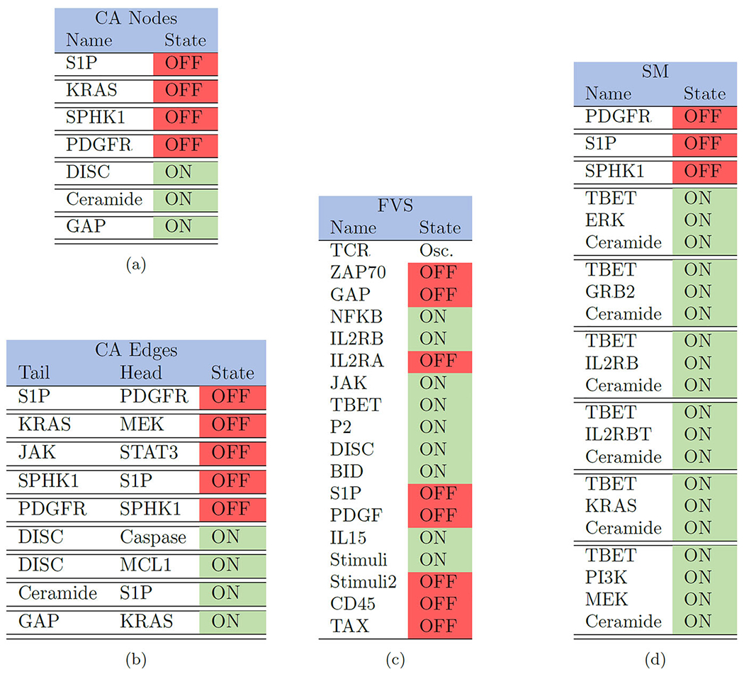
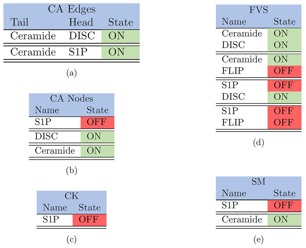
Despite the shared goals of these methods, each seeks distinct control objectives. They are each based on specific mathematical structures and lack a common theoretical framework that allows their complementary and synergistic application. Yet, we clearly see overlapping outcomes between methods. For example, it has been shown that the FVS establishes the upperbound for the magnitude of targets required to control the system (Borriello and Daniels 2021). Indeed, we observe that, among methods using pre-existing attractors, the control sets for CA and SM are subsets of the larger FVS results. On the other hand, CA and CK appear to produce minimal sets. Further, the CA and SM methods can produce the same results, or CA can be a subset of SM. See Tables 2 and 3.

Table 2.

Large T-LGL target tables

Here we list the control targets for the larger T-LGL model, where control sets are separated by double horizontal bars such that (a) (CA Nodes) contains seven singleton controls, (b) (CA Edges) contains nine singleton controls, (c) (FVS) contains one set of 18 controls, and (d) (SM) contains three singleton controls, five triple control sets, and one quadruple control set (Plaugher 2022). Note that some of the larger sets contain elements which are unnecessary due to known singleton controls being a subset of the larger collection. For example, S1P and Ceramide work independently but are also included in larger sets. Further, the CK method did not produce exact results for the large model because of its size (Fig. 2).

Table 3.

Reduced T-LGL target tables

As before, we list the control targets for the small T-LGL model, where control sets are separated by double horizontal bars such that (a) contains two singleton controls, (b) contains three singleton controls, (c) contains one singleton, (d) contains four sets of dual controls, and (e) contains two singleton controls (Plaugher 2022)

However, a key unique feature of CA is the creation of new attractors, while other methods discussed rely on pre-existing attractors. This then leads to the potential for new target discovery as the long-term objectives change. Further, CA sets out to solve a system of polynomial equations, whereas FVS and SM rely on strongly connected components to find their targets. To explicitly see these connections, consider the following example.

2.1. Case Study: T-Cell Large Granular Lymphocyte (T-LGL) Leukemia

T-cell large granular lymphocyte (T-LGL) leukemia is a blood cancer in which there is an anomalous surge in white blood cells, called T-cells. Cytotoxic T-cells are part of the immune system that fight against antigens, even by killing cancer cells. These T-cells release specific cytokines that alter how the immune system responds to external agents by way of recruiting particular immune cells to fight infection, promoting antibody production, or inhibiting the activation and proliferation of other cells (Zañudo and Albert 2015). Once their job is complete they undergo controlled cell-death, however, T-LGL leukemia occurs when these T-cells evade apoptosis and maintain proliferation (Plaugher 2022). There are currently no standards of treatment established, however options include immunosuppressive therapy (such as methotrexate), oral cyclophosphamide (an alkylating agent), or cyclosporine (an immunomodulatory drug) (Loughran 2006). Since there continues to be a search for standard therapies for this disease, the identification of potential therapeutic targets is essential.

In (Saadatpour et al. 2011), a Boolean dynamic model was constructed consisting of a network of sixty nodes indicating the cellular location, molecular components, and conceptual nodes. For the sake of our analysis, we use the Boolean rules in Table 8 (see “Appendix”). The main inputs to the network are “Stimuli”, which represent virus or antigen stimulation, and the main output node is “Apoptosis”. Model analysis revealed that the system contains three attractors, of which two are diseased and the other is healthy (determined by apoptosis activation). Table 2 lists the control targets discovered by each of the respective methods for the large T-LGL model, with the objective of activating apoptosis. Individual control methods are found in Table 2a–d, and control sets are separated by double horizontal bars. Note that the CK method did not produce results for the large model because of its size (Plaugher 2022).

Likewise, an analysis of a smaller (reduced) model of T-LGL can also be useful (Saadatpour et al. 2011; Murrugarra and Aguilar 2018). Model analysis indicated that the reduced model in Fig. 1 contains two fixed points, one healthy and one diseased. Regulatory functions for the small T-LGL model can be found in Appendix Table 7. Table 3a–e list the control targets discovered by each of the respective methods for the small T-LGL model, with the objective of activating apoptosis. The control sets are separated by double horizontal bars as before (Plaugher 2022).

Fig. 1.

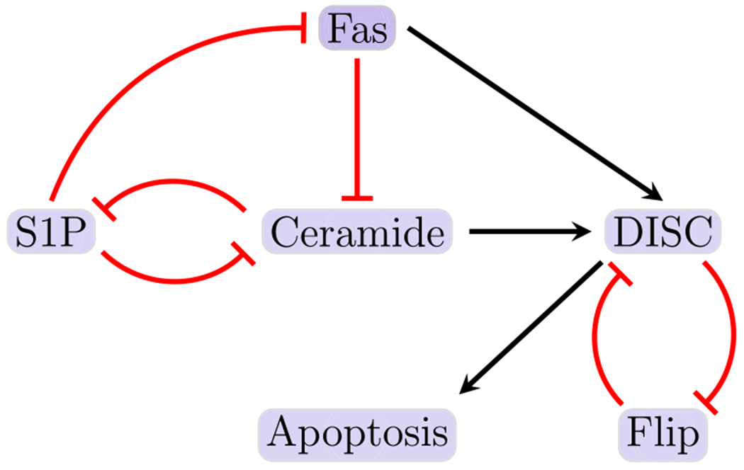
Reduced T-LGL network. The figure shown here indicates the smaller (reduced) T-LGL model, where black barbed arrows indicate signal expression and while red bar arrows indicate suppression (Plaugher 2022) (Color figure online)

For both large and reduced models, we see that FVS provides an upper bound for the amount of targets needed to achieve network control, whereas CA and CK can provide minimal sets.

3. Description of Control Methods

3.1. Computational Algebra (CA)

The method based on computational algebra described in Murrugarra et al. (Sep 2016),Vieira et al. (2020) seeks two types of controls: nodes and edges. These can be achieved biologically by blocking effects of the products of genes associated with nodes, or by targeting specific gene communications (see Fig. 3). The identification of control targets is achieved by encoding the nodes (or edges) of interest as control variables within the functions. Then, the control objective is expressed as a system of polynomial equations that is solved by computational algebra techniques. Though node and edge control are similar, they provide a range of biological options. One reason is that node control requires an entire node to be knocked out (or knocked-in), thereby removing all associated edges (see Fig. 3b). However, edge control simply requires an edge communication to be blocked (or continually expressed) (Plaugher 2022).

Fig. 3.

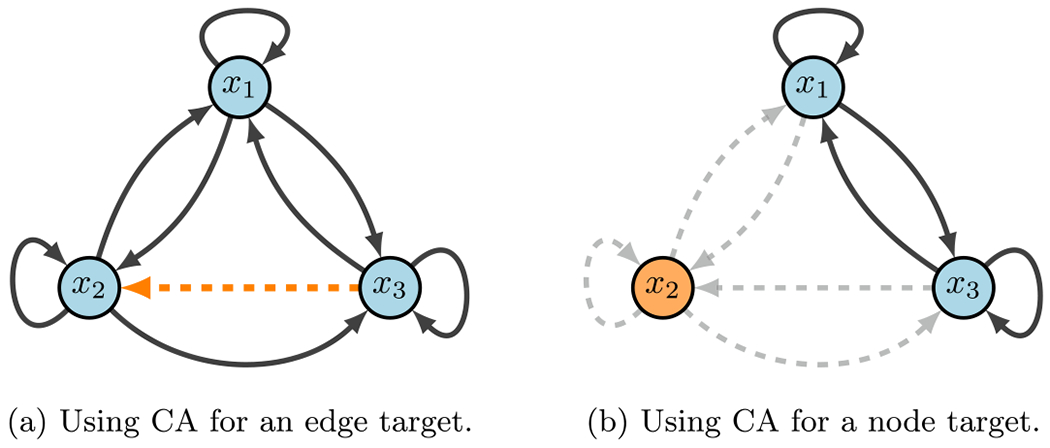
CA diagram. Here, we show a toy model that emphasizes the difference between node and edge control. The key difference with edge control (b), is that all other communications are maintained. Whereas, node control removes every signal associated with the given target

Let the function $ℱ:{\mathbb{F}}_2^n\times U\to {\mathbb{F}}_2^n$ denote a Boolean network with control, where $U$ is a set of all possible controls. Then, for $u\in U$, the new system dynamics are given by $x(t+1)=ℱ(x(t),u)$. That is, each coordinate $u_{i,j}\in u$ encodes the control of edges as follows: consider the edge $x_i\to x_j$ in a given wiring diagram. Then, we can encode this edge as a control edge by the following function:

$${ℱ}_j\left(x,u_{i,j}\right)≔f_j\left(x_1,\dots ,\left(u_{i,j}+1\right)x_i,\dots ,x_n\right)$$

which gives

• Inactive control:

  $$u_{i,j}=0,{ℱ}_j(x,0)=f_j\left(x_1,\dots ,x_i,\dots ,x_n\right)$$
• Active control (edge deletion):

  $$u_{i,j}=1,{ℱ}_j(x,1)=f_j\left(x_1,\dots ,x_i=0,\dots ,x_n\right).$$
  The definition of edge control can therefore be applied to many edges, obtaining $ℱ:{\mathbb{F}}_2^n\times {\mathbb{F}}_2^e\to {\mathbb{F}}_2^n$ where $e$ is the number of edges in the diagram. Next, we consider control of node $x_i$ from a given diagram. We can encode the control of node $x_i$ by the following function:

  $${ℱ}_j\left(x,u_i^{-},u_i^{+}\right)≔\left(u_i^{-}+u_i^{+}+1\right)f_j(x)+u_i^{+}$$

  which yields
• Inactive control:

  $$u_i^{-}=0,u_i^{+}=0,{ℱ}_j(x,0,0)=f_j(x)$$
• Node $x_i$ deletion:

  $$u_i^{-}=1,u_i^{+}=0,{ℱ}_j(x,1,0)=0$$
• Node $x_i$ expression:

  $$u_i^{-}=0,u_i^{+}=1,{ℱ}_j(x,0,1)=1$$
• Negated function value (irrelevant for control):

  $$u_i^{-}=1,u_i^{+}=1,{ℱ}_j(x,1,1)=f_j\left(x_{t_1},\dots ,x_{t_n}\right)+1.$$

  Using these definitions, we can achieve three types of objectives. Let $F=(f_1{}_{,}\dots ,f_n):{\mathbb{F}}_2^n\to {\mathbb{F}}_2^n$ with $\mu =\left\{{\mu }_1,\dots ,{\mu }_n\right\}$ as a set of controls. Then we may:

• Generate new attractors. If $y$ is a desirable state (i.e. apoptosis), but it is not currently an attractor, we find a set $\mu$ that solves

  $${ℱ}_j(y,\mu )-y_j=0,j=1,\dots n$$ (1)
• Block transitions or remove attractors. If $y$ is an undesirable attractor (i.e. proliferation), we want to find a set $\mu$ so that $ℱ(y,\mu )\ne y$. In general, we can use this framework to avoid transitions between states (say $y\to z$) so that $ℱ(y,\mu )\ne z$. We then solve

  $${ℱ}_j(y,\mu )-z_j+1=0,j=1,\dots n$$ (2)
• Block regions. If a particular value of a variable, say $x_k=a$, triggers an undesirable pathway, then we need all attractors to satisfy $x_k\ne a$. A subtle change in notation requires attention, because we have now used $x$ to indicate variables (nodes) rather than specific values (states). We then find a set $\mu$ so that the following system has no solution

  $$\begin{gathered} {ℱ}_j(x,\mu )-x_j=0j=1,\dots n \\ {x}_k-a=0. \end{gathered}$$ (3)

Notably, the Boolean functions $F$ must be written as polynomials (Murrugarra et al. Sep 2016; Vieira et al. 2020). To complete the control search we then compute the Gröbner basis of the ideal associated with the given objective. For example, if we generate new attractors, we find the Gröbner basis for the ideal

$$I=\langle {ℱ}_1(y,\mu )-y_1,\dots ,{ℱ}_n(y,\mu )-y_n\rangle .$$ (4)

Therefore, we can determine all controls that solve the system of equations and detect combinatorial actions for the given model (Plaugher 2022). See “Appendix 7.2.1” for a detailed toy example of the CA method.

3.2. Control Kernel (CK)

A control kernel (CK) is defined as a minimal set of genes (nodes) such that external control of their expression is sufficient to steer the network dynamics toward a desired steady gene activation pattern (attractor) (Borriello and Daniels 2021). In other words, a CK is the set of nodes of minimal magnitude whose pinning reshapes the dynamics such that the basin of attraction of attractor A becomes the entire configuration space. There are three main contributors to the CK: input nodes (nodes with identity function as the updating rule), distinguishing nodes (subset of nodes where a pinning exists that is both compatible with attractor A and incompatible with the other initial attractors of the network), and additional nodes (minimal distinguishing node sets that are needed to remove additional attractors) (Borriello and Daniels 2021; Plaugher 2022).

To compute CKs, first start with pinning input nodes. Then a brute-force method is used to loop over sets of distinguishing nodes of increasing size for each attractor. A CK has been found when no other attractors exist after pinning. Uncontrollable complex attractors are identified by pinning all constant nodes. Note that input and distinguishing nodes provide only a lower bound to CK size because the pinning procedure can create new attractors. If more than one attractor remains, then the cycle does not have a CK (Borriello and Daniels 2021). CK discovery works well for small networks, however, larger networks prove more difficult due to the brute-force nature of the algorithm. In fact, the scaling of the set cardinality is logarithmic based on the number of attractors in the network (Borriello and Daniels 2021; Plaugher 2022). See “Appendix 7.2.2” for a detailed toy example of the CK method.

3.3. Feedback Vertex Set (FVS)

FVS control uses only the topological structure of a network and knowledge of target phenotype biomarkers to induce a phenotype change (Mochizuki et al. 2013; Zañudo et al. 2017). In FVS control, by manipulating the internal state of the feedback vertex set (i.e. a subset of nodes that together intersect every cycle in the network), we disrupt all feedbacks, making the resulting network admit a single steady state, which can be aligned with one of the original system’s dynamic attractors. Thus, a FVS of a graph is a minimal set of nodes whose removal leaves the graph without cycles. FVS control has been successfully applied to a variety of networks and has been shown to provide an upper bound on the cardinality of the single set of control nodes needed to reach all attractors (Borriello and Daniels 2021; Zañudo et al. 2017). The FVS method’s advantages include: (i) control simply requires fixing the internal state of the FVS to match that of the desired attractor, and (ii) making robust predictions that depend only on the network structure and not on dynamical details. For a transcription factor network underlying a phenotypic switch, the FVS is a set of transcription factors that, when controlled to match the expression of a desired phenotype, will shift the cell towards that phenotype (Plaugher 2022).

We formally define a feedback vertex set of a directed graph $W$ as a possibly empty subset $I$ of vertices such that the di-graph $W\setminus I$ is acyclic, where $W\setminus I$ denotes the resulting di-graph when all vertices of $I$ are removed from $W$, along with all edges from or towards those vertices. An alternative way to view FVS is as trees and forests. Recall that a tree is an undirected graph in which any two vertices are connected by exactly one path, that is, a connected acyclic undirected graph. A forest is defined as an undirected graph in which any two vertices are connected by at most one path, that is, an acyclic undirected graph, or a disjoint union of trees (Williamson 2010). Define a graph $G=(V,E)$ that consists of a finite set of vertices $V(G)$ and a set of edges $E(G)$. Then a FVS of $G$ is a subset of vertices $V^{\prime }\subseteq V(G)$ such that the removal of $V^{\prime }$ from $G$, along with all edges incident to $V^{\prime }$, results in a forest (Festa et al. 1999). As such, a FVS must contain all source nodes and a node in every cycle. In other words, a FVS is a set of “determining nodes” such that if the dynamics of the determining nodes are given for large times, then the dynamics of the whole system are determined uniquely for large times (Mochizuki et al. 2013; Fiedler et al. 2013; Plaugher 2022). See “Appendix 7.2.3” for a detailed toy example of the FVS method.

3.4. Stable Motifs (SM)

Stable motif (SM) control is based on the identification of self-sustaining generalized positive feedback loops in the dynamic model. Each of these stable motifs determines a region of the state space from which dynamical trajectories cannot escape, called a trap space. Further, a stable motif (or a succession of multiple stable motifs) determines a dynamical attractor (i.e. phenotype). There is a SM control set associated with each attractor of the system, and the impact of numerous regulators on a single node can be addressed and analyzed with the method (Zañudo and Albert 2015).

By definition, a stable motif is a strongly connected subgraph of the expanded graph (defined subsequently) that (Plaugher 2022):

1. contains either a node or its complement but not both

2. contains all inputs of its composite nodes (if any exist)

First, implement the expanded network that is used to add information about the combinatorial interaction and signs of nodes. Composite nodes represent the AND interaction and complementary nodes represent the NOT interaction. Each original node $i$ is denoted by $x_i$ in the expanded graph, and a complementary node $\left(\sim x_i\right)$ is added if the original node represented suppression. Then, each NOT function is replaced by its appropriate complementary node in the function. Next, edges are included where each edge is a positive regulation, contrary to the original wiring diagram (Yang et al. 2018; Plaugher 2022).

The second step is to make distinctions between OR rules and AND rules by using composite nodes for functions ivolving ANDs. To do this, the functions must be in disjunctive normal form in order to uniquely determine edges. A special node is included for AND rules, and edges are drawn from the non-composite nodes of the network that form the actual composite rule. It is noted that the benefit of such an action is that the reader is able to see all regulatory functions simply from the topology of the expanded network. Now that the expanded graph is complete, using the definition above we can search for SMs within the network. The group of nodes included in the SM represent partial fixed points, from which the remaining nodes can be calculated using the original Boolean functions (Yang et al. 2018; Plaugher 2022). See “Appendix 7.2.4” for a detailed toy example of the SM method.

4. Efficiency Management

In the age of “Big Data”, models are increasingly large and ever more complex. Currently the human genome is estimated to have approximately 25,000 genes, and single genes can encode multiple proteins. What’s more, post-translational modifications add even more complexity to the proteome, with an estimated list of greater than one million proteins (Creative Proteomics 2018). Even networks of merely 100 nodes present a state space of magnitude $2^{100}$, which is much larger than the total estimated cells in the human body (Plaugher 2022). Therefore, the question of control efficiency is an open problem to address. Below, we present possible options for addressing network sizes that are too large for target discovery to be performed in a timely fashion.

4.1. Reduction Techniques

The magnitude of the BN state space for $n$ genes is $2^n$. Thus, an increase of GRN size will exponentially increase the computational burden for its analysis, which means brute-force methods for small systems are not sufficient. A synonymous issue even arises for continuous GRNs. Many reduction techniques allow for the reduction of network size while preserving dynamical features (e.g., fixed points and periodic attractors), see (Veliz-Cuba et al. 2014; Saadatpour et al. 2013). Reduction techniques were implemented in a pancreatic cancer model that effectively decreased the total network size from sixty-nine nodes to twenty-two nodes, a 68% reduction (Plaugher and Murrugarra 2021). Critically, when a node was deleted, its function values were substituted directly into its downstream signal recipient(s) to maintain key network communications. Further, nodes containing self-loops cannot be removed, this includes input (source) nodes and self-modulating nodes.

First, remove nodes with one input and one output, but maintain nodes with self-loops and phenotypes as biomarkers (see Fig.4) (Veliz-Cuba 2011). Next, remove nodes with either one input and multiple outputs, or vice versa (see Fig. 5). Lastly, remove nodes with low connectivity relative to the remaining nodes (see Fig. 6). These techniques have been shown to preserve fixed points but not complex attractors. Yet, there are results indicating a conservation of attractors (Veliz-Cuba et al. 2014; Saadatpour et al. 2013), seen in the preservation of all attractors from the reduced pancreatic cancer model discussed above (Plaugher and Murrugarra 2021). As such, this phenomena remains to be explored.

Fig. 4.

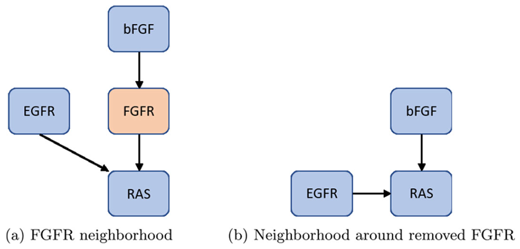
Single-in-single-out removal. Here, we show how to remove FGFR from the network shown in (a) and still maintain downstream signaling shown in (b). See Eqs. (5)–(8) for functional maintenance

Fig. 5.

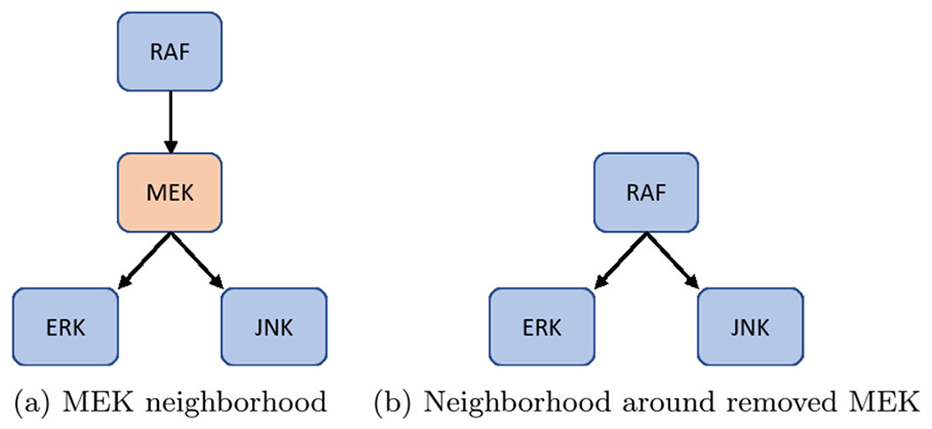
Single-in-multi-out removal. Here, we show how to remove MEK from the network shown in (a) and still maintain downstream signaling shown in (b). See Eqs. (9)–(14) for functional maintenance

Fig. 6.

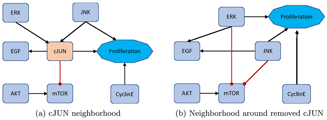
Low connectivity removal. Here, we show how to remove cJUN from the network shown in (a) and still maintain downstream signaling shown in (b). See Eqs. (15)–(22) for functional maintenance

For an example of one input and one output, consider FGFR from the pancreatic cancer model (Plaugher and Murrugarra 2021). The original model’s neighborhood about FGFR is shown in Fig. 4a with Eqs. (5)–(6).

$$\text{FGFR}=\text{bFGF}$$ (5)

$$\text{RAS}=(\mathrm{EGFR})|(\text{FGFR})$$ (6)

After reduction, we obtain the neighborhood seen in Fig. 4b with Eqs. (7)–(8).

$$\sout{\text{FGFR}}=\sout{\text{bFGF}}$$ (7)

$$\text{RAS}=(\mathrm{EGFR})|(\text{bFGF})$$ (8)

For an example of either one input and multiple outputs, or vice versa, consider MEK from (Plaugher and Murrugarra 2021). The original model’s neighborhood about MEK is shown in Fig. 5a with Eqs. (9)–(11).

$$\text{MEK}=\text{RAF}$$ (9)

$$\text{ERK}=\text{MEK}$$ (10)

$$\text{JNK}=\text{MEK}$$ (11)

After reduction, we obtain the neighborhood seen in Fig. 5b with Eqs. (12)–(14).

$$\sout{\text{MEK}}=\sout{\text{RAF}}$$ (12)

$$\text{ERK}=\text{RAF}$$ (13)

$$\text{JNK}=\text{RAF}$$ (14)

Lastly, for an example of multi-connectivity removal, consider cJUN (Plaugher and Murrugarra 2021). The original model’s neighborhood about cJUN is shown in Fig. 6a with Eqs. (15)–(18).

$$\text{cJUN}=(\text{ERK})\mid (\text{JNK})$$ (15)

$$\text{EGF}=\text{cJUN}$$ (16)

$$\text{mTOR}=(\sim \text{cJUN})\&(\text{AKT})$$ (17)

$$\text{Pro}=(\text{CyclinE})\&((\text{JNK})\mid (\text{cJUN}))$$ (18)

After reduction, we obtain the neighborhood seen in Fig. 6b with Eqs. (19)–(22).

$$\sout{\text{cJUN}}=\left(\sout{\text{ERK}}\right)|\left(\sout{\text{JNK}}\right)$$ (19)

$$\text{EGF}=(\text{ERK})\mid (\text{JNK})$$ (20)

$$\text{mTOR}=(\sim [(\text{ERK})\mid (\text{JNK})])\&(\text{AKT})$$ (21)

$$\text{Pro}=(\text{CyclinE})\&((\text{JNK})|(\text{ERK})|(\text{JNK}))$$ (22)

4.2. Modularity Techniques

Systems biology is capable of building complicated structures from simpler building blocks, even though these simple blocks (i.e. modules) traditionally are not clearly defined. The concept of modularity detailed in Kadelka et al. (2022) is structural by nature, in that, a module of a BN is a subnetwork in which the restriction of the network to the variables of a subgraph has a strongly connected wiring diagram. This framework introduces both a structural and dynamic decomposition that encapsulates the dynamics of the whole system simply from the dynamics of its modules. Consequently, the decomposition yields a hierarchy among modules that can be used to specify controls. That is, by controlling key modules we are able to control the entire network (Plaugher 2022).

Within the modularity framework, the dynamics of the state-space for Boolean network $F$ are denoted as $𝒟(F)$, which is a collection of all minimal subsets of attractors, $A$, satisfying $F(A)=A$. Further, if $F$ is decomposable (say into subnetworks $H$ and $G$), then we can write $F=H⋊G$ which is called the coupling of $H$ and $G$. In the case where the dynamics of $G$ are dependent on $H$, we call $G$ non-autonomous, denoted as $\overline{G}$. Then we adopt the following notation: let $A=A_1\oplus A_2$ be a set of attractors of $F$ with $A_1\in 𝒟(H)$ and $A_2\in 𝒟\left(G^{A_1}\right)$ (Plaugher 2022).

For an example, consider the network in Fig. 7a with

$$F\left(x_1,x_2,x_3,x_4,x_5,x_6\right)=\left(x_3,x_1,x_2,x_1{x}_6,x_4,x_5\right).$$

Fig. 7.

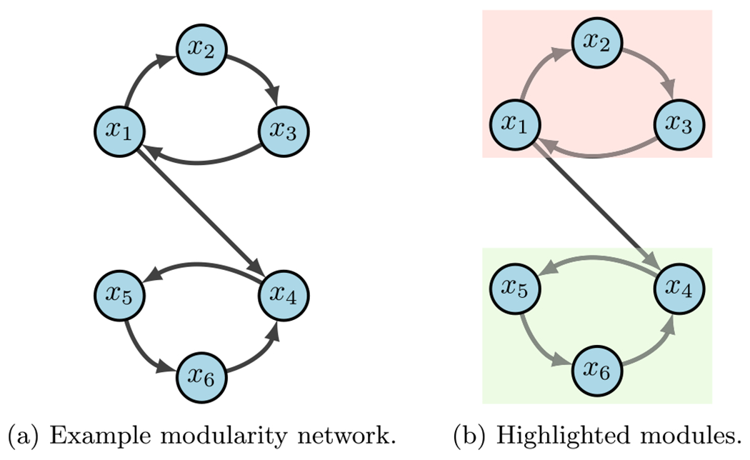
Modularity example (Plaugher 2022)

From the given wiring diagram, we derive two SCCs where module one (red in 7b) flows into module two (green in 7b). That is, $F=F_1⋊F_2$ with

$$F_1\left(x_1,x_2,x_3\right)=\left(x_3,x_1,x_2\right)$$

$$F_2\left(x_4,x_5,x_6\right)=\left(x_6,x_4,x_5\right)$$

$$\overline{F_2}\left(x_4,x_5,x_6\right)=\left(x_1{x}_6,x_4,x_5\right)$$

$$𝒟\left(F_1\right)=\{000,111,[001,100,010],[011,101,110]\}$$

Suppose we aim to stabilize the system into $y=000000$. First we see that either $x_1=0,x_2=0x_2=0,$ or $x_3=0$ stabilize module one (i.e. $F_1$) to $A_1=000$ by applying the FVS method from Sect. 3.3. Likewise, $x_4=0,x_5=0$ or $x_6=0$ stabilize module two (i.e. $F_2^{A_1}$) to $A_2=000$. Thus, we can conclude that $u=\left(x_1=0,x_6=0\right)$ is a possible combinatorial solution that achieves the desired result (Plaugher 2022).

5. Limitations

5.1. Validation

Even though phenotype control theory shows massive potential, the field overall has some limitations, along with those of each technique we have described. From a biological and translational perspective, it remains yet to be validated as a viable option for clinical application. Further, the human genome is highly complex, with signaling mechanisms that are far from well understood. This leads modelers to rely on speculative networks and hypothesized functional communication rules.

Regardless of method, each of the resulting outputs are merely theoretical controls and must be parsed to find tangible targets (or combinations of targets). Efficacy of the resulting targets can be established computationally, which is discussed in the “Appendix 7.3”. The parsing process can include brute-force testing of all controls, knowledge of the regulatory network topology, knowledge of literature pertaining to particular controls, or a mixture of various techniques (Murrugarra et al. Sep 2016; Plaugher et al. 2022). Some controls may not be biologically achievable, others may be insufficient if applied independently, while some simply do not perform as desired.

5.2. Methodological Unification

Since we do not apply optimal control, another constraint to address is how to select controls that prioritize certain interventions over others. These criteria might include selection according to effectiveness (e.g. shorter absorption time), total/side effects (e.g. number of changes in the original state space), target “depth” within the network, and practical implementability. Many of the selection criteria will need stochasticity (such as for time to absorption), which can be achieved via Stochastic Discrete Dynamical Systems (SDDS) (Murrugarra et al. 2012, 2016) or asynchronous simulations (see “Appendix 7.1” for more details). The SDDS framework incorporates Markov chain (MC) tools to study long-term dynamics of Boolean networks by merging the synchronous and asynchronous update schedules to encode a more realistic MC.

When it comes to network reduction, techniques can prove extremely tedious if networks are notably large. Further, the reduction techniques can change the long-term outlooks of key analytical features such as cyclical attractors. It has been shown that the methods in Sect. 4.1 will maintain fixed points, but they do not necessarily maintain cyclical attractors (Veliz-Cuba et al. 2014; Saadatpour et al. 2013; Plaugher and Murrugarra 2021). Even though examples have been shown to maintain all attractors (Plaugher and Murrugarra 2021; Plaugher 2022), one can easily show counter examples that do not (see the small T-LGL model in Sect. 2.1). Thus, a fully developed methodology for efficient reduction is yet to be seen, which could be important for analyzing large models.

5.3. Computational Complexity

Additionally, computational complexity varies across methods. For instance, the CA method makes use of computing Gröbner bases for a system of polynomials and, depending on the algorithm used, it has been shown to have doubly exponential complexity (Murrugarra et al. Sep 2016). However, GRNs with small sets of regulatory nodes can compute Gröbner bases in a reasonable time (Murrugarra et al. Sep 2016; Hinkelmann et al. 2011).

For CK, the problem of finding the minimal set of controlling nodes was shown to be NP-hard (Akutsu et al. 2007), and the problem of the existence of multiple possible minimal control sets is NP-complete. Thus, when computing CKs, no algorithm is expected to run faster in the worst case than checking every possible subset of increasing size, since the rounds of pinning to find CK’s are representative of NP-hard problems. Moreover, the average CK sizes scale logarithmically with the number of attractors (Borriello and Daniels 2021).

The computational time to find a single FVS is reasonable, the issue arises when trying to find all possible FVSs. The global stabilization of BNs have been shown to have computational complexity that is exponential with respect to the number of state variables (Cheng et al. 2011; Yang et al. 2021). However, while the problem of exactly identifying the minimal FVS has complexity of NP-hard, a variety of fast algorithms exist to find close-to-minimal solutions (Zañudo et al. 2017; Galinier et al. 2013).

Lastly, the complexity of calculating SMs using the domain of influence (DOI), through the expanded graph (Yang et al. 2018), is bounded by the order of the sum the number of nodes and edges in the expanded network, $O\left(N_{ex}+E_{ex}\right)$. Subsequent calculations for finding control sets from the DOI become more complex. So called “well behaved degree distribution” networks give calculated order $O\left(k^2{N}^2\right)$, where $k$ are the regulators for each node $N$. Those networks considered to have “skewed degree distribution” are bounded by $O(N^3)$ (Yang et al. 2018).

6. Conclusions

In this paper, we reviewed various techniques for implementing target discovery and control of gene regulatory networks. Due to the growing nature of the field, there are always emerging, novel techniques to implement and we acknowledge that the methods included here are not fully exhaustive (Cifuentes-Fontanals et al. 2022, ?; Murrugarra and Dimitrova 2015; Yang et al. 2020; Murrugarra and Dimitrova 2021). Even so, we have set out to provide a list of varying options, depending on the specific aims and information available to users, that represent a broad range of applicable theory. We also hope to spark conversations and ideas for solving open problems in the field, as well as inspire application of these concepts across a wide range of disciplines, not strictly biology. For links to software and documentation, see “Appendix 7.4”.

In addition to toy examples for each method (see “Appendix 7.2”), we also applied each approach to a well known cancer model (T-LGL Leukemia) to explore overlaps and differences among the processes. In particular, we showed that FVS provides an upper bound for the amount of targets needed to achieve network control, whereas CA and CK can provide minimal sets. Perhaps the most versatile method shown is CA, where users have wide ranging options to personalize their search (i.e. nodes vs. edges, use existing attractors, generate new attractors, and block transitions or regions). These overlaps have also been shown in a computational pancreatic cancer model (Plaugher and Murrugarra 2021; Plaugher et al. 2022).

Even though there is not a common theoretical framework to apply all methods, we do see that each is capable of affirming discoveries across other methods while also suggesting possible novel targets of their own. We believe the future is bright for synthetic modeling and control of cell signaling networks, and the methods reviewed herein are just the beginning.

Fig. 2.

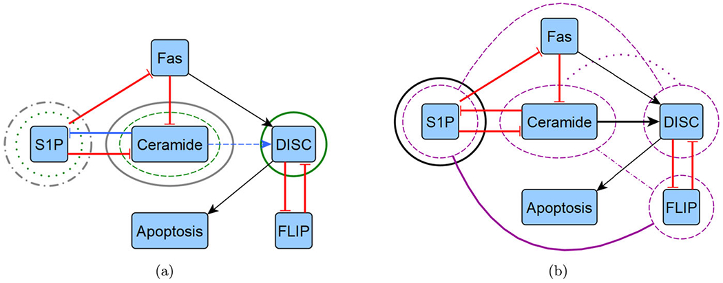
Reduced T-LGL network target overlaps. We highlight the overlapping control targets from Table 3 by overlaying them with the reduced T-LGL wiring diagram from Fig. 1, shown in two diagrams for clarity. a We show instances of CA edge (blue), CA node (green), and SM (grey). b We show instances of CK (black) and FVS (purple). Note that FVS has combinatorial controls with connecting arches, where others are strictly singleton (Color figure online)

Appendix

7. Appendix

7.1. Finite Dynamical Systems

For the last few decades, a popular modeling approach for gene regulation has been to implement dynamical systems over finite fields. Here, functions can be interpreted as modeling information processing within cells, which determines cellular behavior. As depicted in Fig. 8, $\left\{x_{i_1},\dots ,x_{i_m}\right\}$ represent the input genes or predictor genes, $f_i\left(x_{i_1},\dots ,x_{i_m}\right)$ is the internal update function or predictor rule, and $x_i$ is the target gene.

Fig. 8.

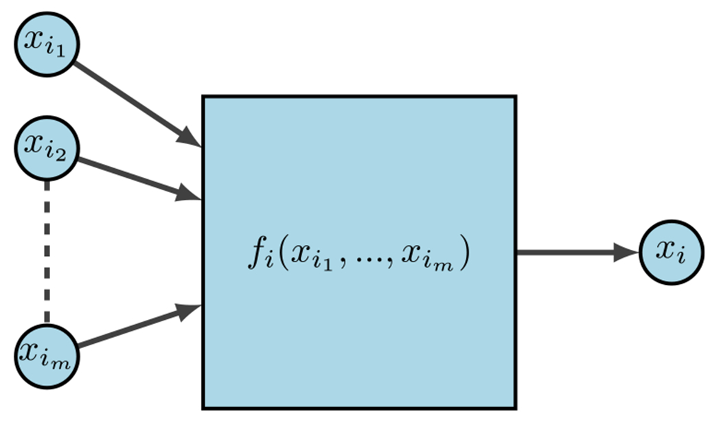
FDS for gene regulation (Plaugher 2022)

First, let $X=X_1\times X_2\cdots \times X_n$ be the Cartesian product of finite sets. A local model over a finite set $X$ is an n-tuple of coordinate functions $F=\left(f_1,f_2\dots ,f_n\right)$, where $f_i:X^n\to X$. Each function $f_i$ uniquely determines a function

$$F_i:\left(x_1,\dots ,x_n\right)\mapsto \left(x_1,\dots ,f_i(x),\dots ,x_n\right)$$

and $x=\left(x_1,\dots ,x_n\right)$. Every local model defines a canonical finite dynamical system $\left(FDS\right)$ map, where the functions are updated as

$$f:X^n\to X^n,f:\left(x_1,\dots ,x_n\right)\mapsto \left(f_1(x),\dots ,f_n(x)\right).$$

Note that discrete does not necessarily imply finite. Take the natural numbers $\mathbb{N}=1,2,3,4$, … , for example. The set is clearly discrete, yet its cardinality is infinite. In general, we cannot always write a function as a tuple if the space is simply “discrete”. In order to provide structure to each $X_i$, we embed $X_i$ into a finite field where, for some prime $p$,

$$X_i\hookrightarrow \mathbb{F},|\mathbb{F}|=p^k.$$

For example, if we desire states of Low, Medium, and High to represent levels of gene expression, then $X_i=\{L,M,H\}\hookrightarrow {\mathbb{F}}_3=\{0,1,2\}$. We call these mixed-state models when states are non-binary. For the case when all states are binary (i.e. ON or OFF, HIGH or LOW, 1 or 0), we call these models Boolean networks (Plaugher 2022).

7.1.1. Boolean Networks

Boolean networks (BNs) are popular because we can build effective models without the use of constants or rates. This then eliminates the need for tedious parameter discovery. Rather, BNs focus on the mechanics and logic of the system. BN models were originally introduced in 1963 by Kauffman and Thomas to provide a coarse grained description of gene regulatory networks (Kauffman 1969; Thomas 1973). Within a BN there are three main components: structure (wiring diagram), functions (regulatory rules), and dynamics (attractors). As we begin to define our terms, it may be helpful to keep Fig. 9 in mind as a basic example. Given $n$ binary variables, define a Boolean Network as an $n$-tuple of coordinate functions

$$F=\left(f_1,\dots f_n\right):{\{0,1\}}^n\to {\{0,1\}}^n,f_i:{\{0,1\}}^n\mapsto \{0,1\}.$$

Fig. 9.

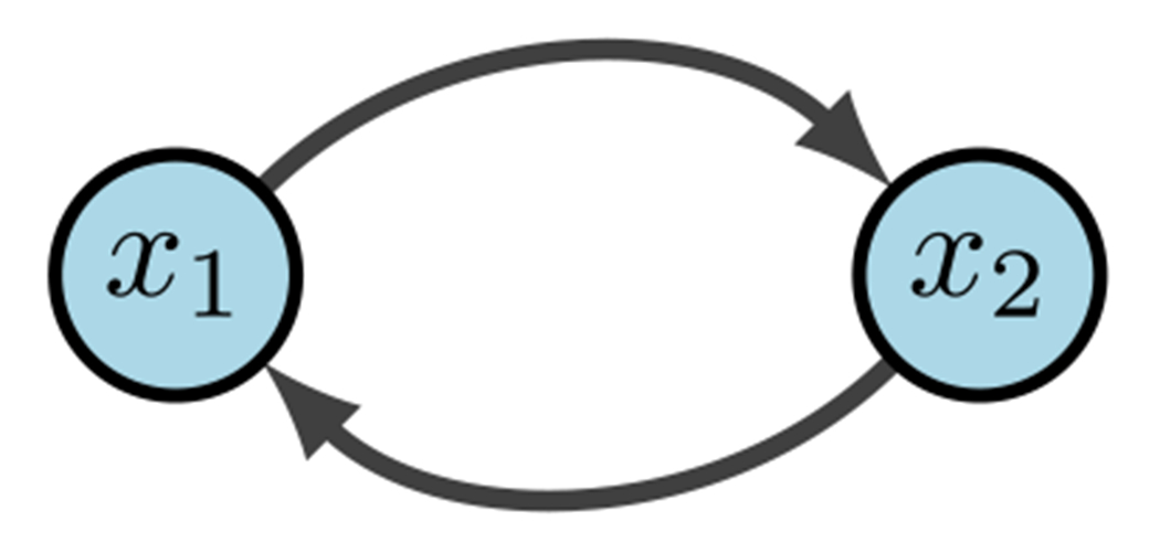
Simple Boolean network (Plaugher 2022)

The wiring diagram of $F$, call it $W$, is then defined as a directed graph with $n$ nodes $\left\{x_1,x_2,\dots ,x_n\right\}$ such that there is an edge in $W$ from $x_j$ to $x_i$ if $f_i$ depends on $x_j$. That is,

$$x_j\to x_i\text{if}{f}_i=f\left(x_{i_1},\dots ,x_{i_j},\dots ,x_{i_k}\right)$$

Within $W$ we denote positive edges as $x_j\to x_i$ and negative edges as $x_j⊣x_i$ (or sometimes $x_j⊸x_i$). Biologically, a positive edge is representative of activation while a negative edge represents inhibition. For example, in Fig. 9 we see the wiring diagram of $F=\left(f_1,f_2\right)=\left(x_2,x_1\right)$.

Now that we have structure and functions, the dynamics of $F$ are traditionally described as: (1) trajectories for all $2^n$ possible initial conditions, or (2) a directed graph with nodes in ${\mathbb{F}}_2^n={\{0,1\}}^n$. In the first case, a trajectory is a sequence ${(x(t))}_{t=0}^{\infty }$ given by the difference equations $x(t+1)=F(x(t))$ for all $t\ge 0$ (Kadelka et al. 2022). For example, Fig. 9 would yield deterministic trajectories

$$\begin{gathered} T_1=\left(00,00,00,\dots \right) \\ {T}_2=\left(11,11,11,\dots \right) \\ {T}_3=\left(01,10,01,10,\dots \right) \\ {T}_4=\left(10,01,10,01,\dots \right). \end{gathered}$$

The phase space (also called state space) of $F$ is the directed graph with vertex set $S^n$ and edge set $\left\{(s,f(s))\mid s\in S^n\right\}$. Simply put, in a BN, $S$ is the set of all possible states, and their respective transitions according to the model $F$ form the state space (see Fig. 10). A node $s\in S$ is called transient if $f^k(s)\ne s$ for all $k>1$, a node $s\in S$ is called periodic (or cyclic) if $f^k(s)=s$ for some $k\ge 1$, and a node $s\in S$ is called a fixed point if $f(s)=s$. We can also think of the phase space as having strongly connected components (SCCs), where a SCC is said to be terminal if it has no out-going edges. Thus, a transient state is not in a terminal SCC, a cyclic attractor is in a terminal k-cycle ($k=1$ is a fixed point), and any instance of an SCC otherwise is a complex attractor. In other words, we define an attractor as a set of states from which there is no escape as the system evolves, and an attractor with a single state is called a fixed point. Thus, given sufficient time, the dynamics of a BN always end up in a fixed point or (complex) attractor.

Fig. 10.

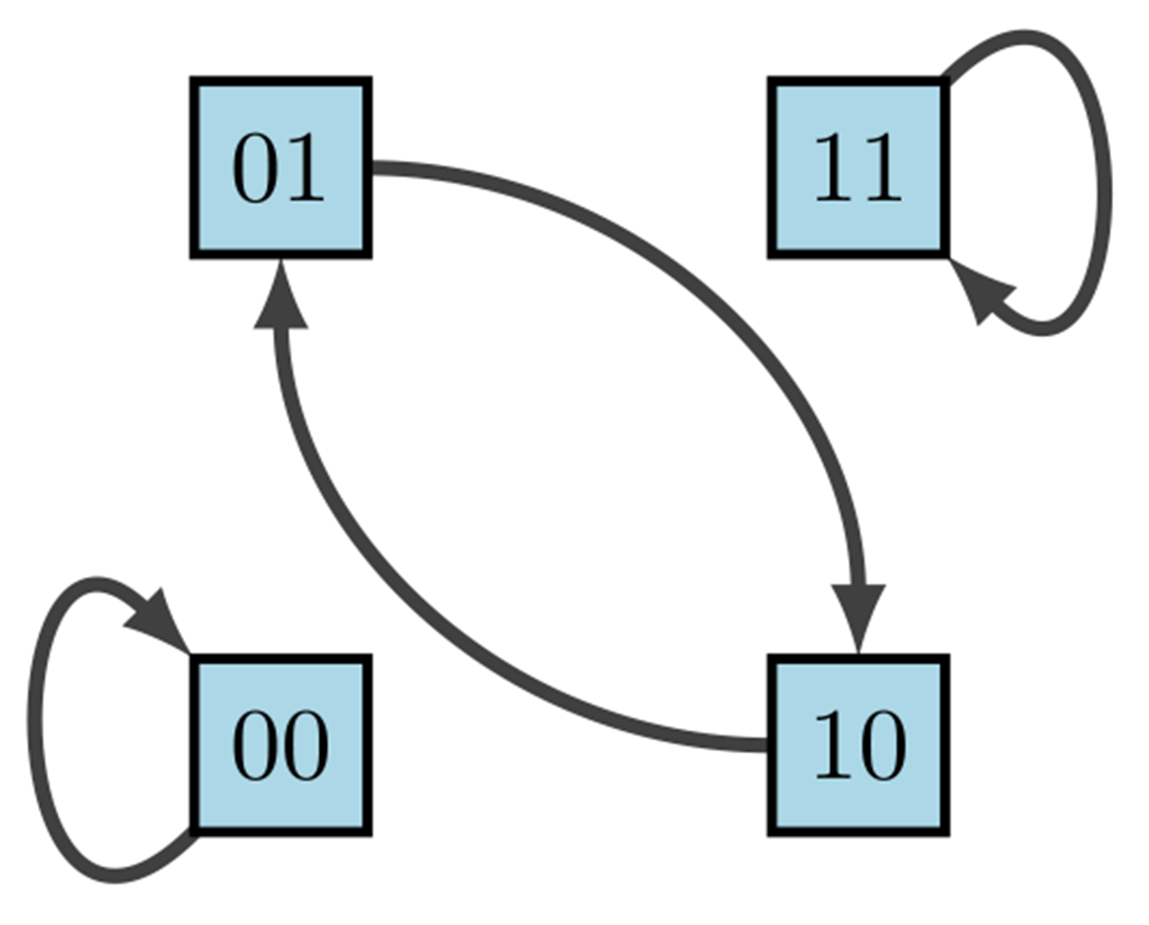
Phase space of diagram 9 (Plaugher 2022)

Table 4.

Dynamic truth table for Fig. 9

$x_1$	$x_2$	$f_1=x_2$	$f_2=x_1$
0	0	0	0
0	1	1	0
1	0	0	1
1	1	1	1

Fig. 11.

Nonlinear Boolean network (Plaugher 2022)

Table 5.

Standard Boolean logical rules

Rule	Symbol	Polynomial
AND	$x\wedge y,x\&y$	$xy$
OR	$x\vee y,x|y$	$xy+x+y$
NOT	$\left(\sim x\right),\overline{x},\left(\neg x\right)$	$x+1$

For example, it was previously shown above that $F=\left(f_1,f_2\right)=\left(x_2,x_1\right)$. To find the dynamics of the corresponding state space $S=\{00,01,10,11\}$, one can construct truth Table 4 using lexicographic ordering. It is important to point out that we denote the states in order of the variable so that

$$s_2=\{0,1\}=01=\left\{x_1=0,x_2=1\right\},$$

because maintaining order is highly important for correct interpretation of state values. The left columns indicate the possible states of our nodes $x_1$ and $x_2$, whereas the right columns indicate their deterministic updates according to the functions $f_1$ and $f_2$. Therefore, from the framework we see in Fig. 10 that we have two fixed points and one cycle.

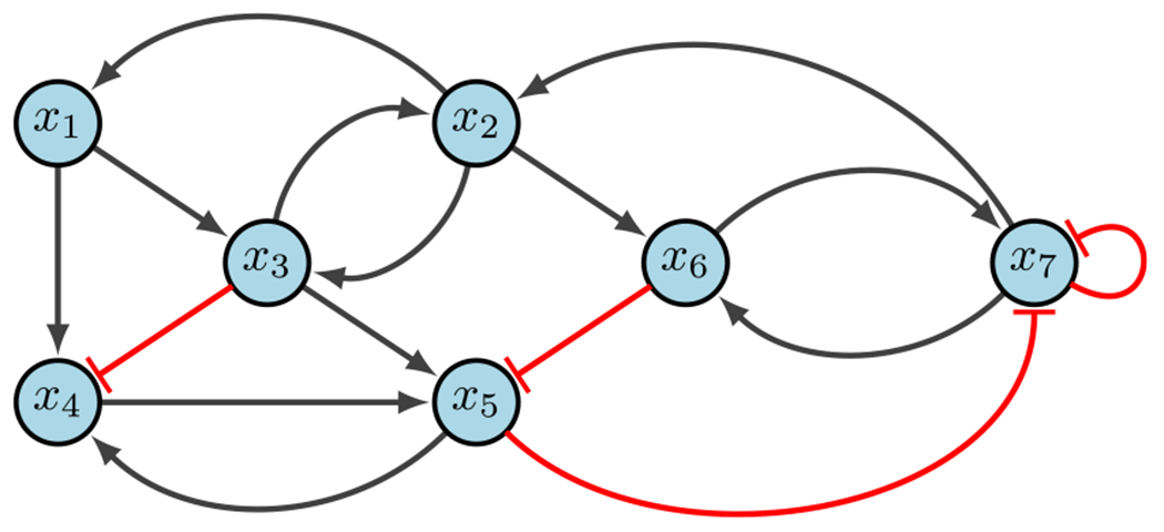
Up to this point we have only discussed linear BNs, but real-world models are almost always highly nonlinear (see Fig. 11). To accommodate these nonlinear regulatory networks, we implement various classes of functions based on three main Boolean logical rules - AND, OR, NOT. Some use XOR (exclusive OR), but for simplicity it is excluded here. Assume the variables $x$ and $y$ are given in a BN. Then Table 5 summarizes the functionality and notation used for each of the three main rules.

Fig. 12.

State-space dynamical variants according to update schedules (Plaugher 2022)

A common criticism of using discrete models for regulatory networks such as BNs is that deterministic dynamics are artificial. In reality biological systems do not contain a “central clock”, but instead the concentration levels of gene products change and respond to stimuli on varying time-scales. Thus, the update schedules chosen play a significant role in the accuracy of the model. Synchronous update schedules produce deterministic dynamics, wherein nodes are all updated simultaneously so that

$$x(0)\to x(1)=F(x(0))\to x(2)=F(x(1))\to \cdots .$$

On the other hand, asynchronous update schedules produce stochastic dynamics, wherein a randomly selected node is updated at each time step so that

$$x(0)\to x(1)=\left(x_1(0),\dots ,f_i(x(0)),\dots ,x_n(0)\right)\to \cdots .$$

Lastly, sequential update schedules are performed asynchronously according to a designated permutation $\sigma =\left({\sigma }_1,\dots ,{\sigma }_n\right)$ of $(1,\dots ,n)$. Specifically, if we define $F_i\left(x_1,\dots ,x_n\right)=\left(x_1,\dots ,f_i(x),\dots ,x_n\right)$, then the update is given by

$$F_{\sigma }(x)=F_{{\sigma }_n}\left(F_{{\sigma }_{n-1}}\left(\cdots \left(F_{{\sigma }_1}(x)\right)\cdots \right)\right)$$

according to the order designated by $\sigma$. This is sometimes done when the ordering of gene updates are known, as some may update faster than others. For example, using our simple example in Figs. 9, 12 shows the varying impacts of these three update schedules.

We can easily observe from Fig. 12 that fixed points are maintained across all update schedules. However, cycles are not necessarily preserved. As a result, different update schedules lead to different dynamics in the state space, which could lead to different attractors (or eliminate attractors), which would result in different target discoveries for interventions. This is where the framework of Stochastic Discrete Dynamical Systems (SDDS) is beneficial (Murrugarra and Aguilar 2018; Plaugher and Murrugarra 2021; Plaugher et al. 2022; Plaugher 2022). Developed in Murrugarra and Aguilar (2018), SDDS incorporates Markov chain tools to study long-term dynamics of Boolean networks. SDDS uses parameters based on designated propensities to model node (and pathway) signal activation and deactivation, also referred to as degradation. In essence, SDDS merges the synchronous and asynchronous update schedules described above. One propensity is used when the update positively impacts the node, in the sense that the node increases its value from OFF to ON. Another propensity is used when the update negatively affects the node in the sense that the node decreases its value from ON to OFF. More precisely, an SDDS of the variables $\left(x_1,x_2,\dots ,x_n\right)$ is a collection of $n$ triples

$$\hat{F}={\left\{f_k,p_k^{\uparrow },p_k^{\downarrow }\right\}}_{k=1}^n$$

where for $k=1,\dots ,n,$

• $f_k:{\{0,1\}}^n\to \{0,1\}$ is the update function for $x_k$

• $p_k^{\uparrow }\in [0,1]$ is the activation propensity

• $p_k^{\downarrow }\in [0,1]$ is the deactivation propensity

Here, the parameters $p_k^{\uparrow }$ and $p_k^{\downarrow }$ introduce stochasticity. For example, an activation of $x_k(t)$ at the next time step (i.e. $x_k(t)=0,f_k\left(x_1(t),\dots ,x_n(t)\right)=1$ and $x_k(t+1)=1$) occurs with probability $p_k^{\uparrow }$. An SDDS can be represented as a Markov Chain via its transition matrix, which can be viewed as transition probabilities between various states of the network. Elements of the transition matrix $A$ are determined as follows: consider the set $S={\{0,1\}}^n$ consisting of all possible states of the network. Suppose $x=\left(x_1,\dots ,x_n\right)\in S$ and $y=\left(y_1,\dots ,y_n\right)\in S$. Then, the probability of transitioning from $x$ to $y$ is

$$a_{y,x}=\prod _{i=1}^{n}P\left(x_i\to y_i\right)$$ (23)

where entries are stored column-wise and

$$P\left(x_i\to f_i(x)\right)=\{\begin{array}{c}{p}_k^{\uparrow },\text{if}{x}_i<f_i(x)\\ p_k^{\downarrow },\text{if}{x}_i>f_i(x)\\ 1,\text{if}{x}_i=f_i(x)\end{array}\mathrm{and}P\left(x_i\to x_i\right)=\{\begin{array}{c}1-p_k^{\uparrow },\text{if}{x}_i<f_i(x)\\ 1-p_k^{\downarrow },\text{if}{x}_i>f_i(x)\\ 1,\text{if}{x}_i=f_i(x)\end{array}.$$

It follows that $P\left(x_i\to y_i\right)=0$ for any $y_i\notin \left\{x_i,f_i(x)\right\}$. Therefore, we achieve $A={\left[a_{y,x}\right]}_{x,y\in S}$. Note that when propensities are set to $p=1$, we have a traditional BN. With this framework, we built a simulator that takes random initial states as inputs and then tracks the trajectory of each node through time. Long-term phenotype expression probabilities can then be estimated, as well as network dynamics with (and without) controls (Plaugher 2022).

Fig. 13.

CA example (Plaugher 2022)

7.2. Elementary Examples for Control Methods

7.2.1. Computational Algebra

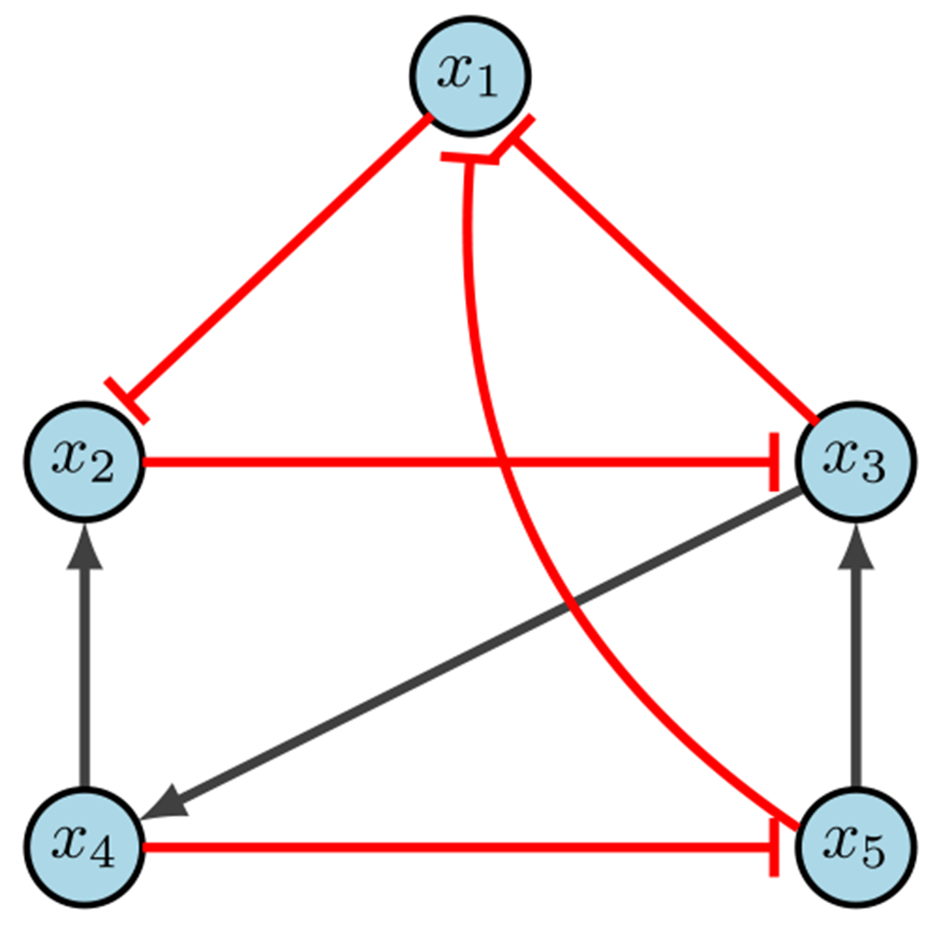
Consider the network in Fig. 13, with the following regulatory functions.

$$\begin{gathered} f_1=\left(\sim x_3\right)\wedge \left(\sim x_5\right) \\ {f}_2=\left(\sim x_1\right)\vee x_4 \\ {f}_3=\left(\sim x_2\right)\vee x_5 \\ {f}_4=x_3 \\ {f}_5=\sim x_4 \end{gathered}$$

Using Table 5, we rewrite our functions as the following simplified polynomials.

$$\begin{gathered} f_1=1+x_3+x_5+x_3{x}_5 \\ {f}_2=1+x_1+x_1{x}_4 \\ {f}_3=x_2{x}_5+x_2+1 \\ {f}_4=x_3 \\ {f}_5=1+x_4 \end{gathered}$$

We can then find the fixed points of the system by solving $f_i=x_i$ for $i=1,\dots ,5$. Another way to view this step is as finding roots of $g_i=0$ where $g_i=f_i-x_i$, then finding the Grobner basis of the ideal $I=\langle g_1,\dots ,g_5\rangle$. In any case, the example in Fig. 13 does not contain any fixed points. However, further state space analysis does reveal two attractors: $\{01011,01100\}$ and $\{00101,01010,01110,01111,10001,11000\}$. Now, we encode our edge controls as

$$\begin{gathered} {ℱ}_1=1+\left(u_{3,1}+1\right)x_3+\left(u_{5,1}+1\right)x_5+\left(u_{3,1}+1\right)x_3\left(u_{5,1}+1\right)x_5 \\ {ℱ}_2=1+\left(u_{1,2}+1\right)x_1+\left(u_{1,2}+1\right)x_1\left(u_{4,2}+1\right)x_4 \\ {ℱ}_3=\left(u_{2,3}+1\right)x_2\left(u_{5,3}+1\right)x_5+\left(u_{2,3}+1\right)x_2+1 \\ {ℱ}_4=\left(u_{3,4}+1\right)x_3 \\ {ℱ}_5=1+\left(u_{4,5}+1\right)x_4 \end{gathered}$$ (24)

and node controls as

$$\begin{gathered} {ℱ}_1=\left(u_1^{-}+u_1^{+}+1\right)\left(1+x_3+x_5+x_3{x}_5\right)+u_1^{+} \\ {ℱ}_2=\left(u_2^{-}+u_2^{+}+1\right)\left(1+x_1+x_1{x}_4\right)+u_2^{+} \\ {ℱ}_3=\left(u_3^{-}+u_3^{+}+1\right)\left(x_2{x}_5+x_2+1\right)+u_3^{+} \\ {ℱ}_4=\left(u_4^{-}+u_4^{+}+1\right)x_3+u_4^{+} \\ {ℱ}_5=\left(u_5^{-}+u_5^{+}+1\right)\left(1+x_4\right)+u_5^{+}. \end{gathered}$$ (25)

Let’s consider the objective of generating new attractors, and assume we want our steady state to be $y=11110$. In general, one can search the entire system for controls, but there may be special cases where limiting decisions can be made amongst collaborators. For arguments sake, suppose we want to find edge knockouts and limit our search to edges $x_3\to x_1,x_5\to x_1$, and $x_2\to x_3$. Then the updated edge equations (Eq. 24) become

$$\begin{gathered} {ℱ}_1=1+\left(u_{3,1}+1\right)x_3+\left(u_{5,1}+1\right)x_5+\left(u_{3,1}+1\right)x_3\left(u_{5,1}+1\right)x_5 \\ {ℱ}_2=1+x_1+x_1{x}_4 \\ {ℱ}_3=\left(u_{2,3}+1\right)x_2{x}_5+\left(u_{2,3}+1\right)x_2+1 \\ {ℱ}_4=x_3 \\ {ℱ}_5=1+x_4. \end{gathered}$$ (26)

Evaluating at $y=11110$ yields

$${ℱ}_1=u_{3,1},{ℱ}_2=1,{ℱ}_3=u_{2,3},{ℱ}_4=1,{ℱ}_5=0.$$

Therefore, the desired fixed point is achieved if and only if $u_{3,1}=u_{2,3}=1$. That is, the controls for $u_{3,1}$ and $u_{2,3}$ are active, such that we must delete both corresponding edges. Similarly, we can determine node control to achieve new fixed point $y=11110$. Again, for simplicity, we limit ourselves to $x_1$ knock-in, $x_3$ knock-out and knock-in, and $x_4$ knock-in. The updated node equations (Eq. 25) then become

$$\begin{gathered} {ℱ}_1=\left(u_1^{+}+1\right)\left(1+x_3+x_5+x_3{x}_5\right)+u_1^{+} \\ {ℱ}_2=1+x_1+x_1{x}_4 \\ {ℱ}_3=\left(u_3^{-}+u_3^{+}+1\right)\left(x_2{x}_5+x_2+1\right)+u_3^{+} \\ {ℱ}_4=\left(u_4^{+}+1\right)x_3+u_4^{+} \\ {ℱ}_5=1+x_4. \end{gathered}$$ (27)

Evaluating at $y=11110$ yields

$${ℱ}_1=u_1^{+},{ℱ}_2=1,{ℱ}_3=u_3^{+},{ℱ}_4=1,{ℱ}_5=0.$$

Thus, the desired fixed point is achieved if and only if $u_1^{+}=1$ and $u_3^{+}=1$. Importantly, this means that the controls by themselves are insufficient but together they achieve the desired goal. One can easily see that requiring numerous controls in much larger systems may not be biological feasible, which is why alternate objectives can prove useful.

Suppose we determine that $y=01111$ is in a diseased attractor which we want to destroy. We can then aim to block the transition from $y$ to $F(y)=01110$. We limit ourselves to considering edges from $x_3\to x_1,x_5\to x_1,x_3\to x_4$, and $x_4\to x_5$. The updated edge equations (Eq. 24) become

$$\begin{gathered} {ℱ}_1=1+\left(u_{3,1}+1\right)x_3+\left(u_{5,1}+1\right)x_5+\left(u_{3,1}+1\right)x_3\left(u_{5,1}+1\right)x_5 \\ {ℱ}_2=1+x_1+x_1{x}_4 \\ {ℱ}_3=x_2{x}_5+x_2+1 \\ {ℱ}_4=\left(u_{3,4}+1\right)x_3 \\ {ℱ}_5=1+\left(u_{4,5}+1\right)x_4. \end{gathered}$$ (28)

Evaluating at $y=01111$ yields

$${ℱ}_1=u_{3,1}{u}_{5,1},{ℱ}_2=1,{ℱ}_3=1,{ℱ}_4=u_{3,4}+1,{ℱ}_5=u_{4,5}.$$

This means that Eq. 2 becomes

$$\left(u_{3,1}{u}_{5,1}+1\right)\left(u_{3,4}\right)\left(u_{4,5}+1\right)=0$$

giving three possible solutions: $u_{3,1}=u_{5,1}=1,u_{3,4}=0$, or $u_{4,5}=1$. Notice that we again have a combinatorial solution in $u_{3,1},u_{5,1}$ since they are insufficient individually but successful together, $u_{3,4}=0$ means that the control is inactive, and $u_{4,5}$ is a singleton control.

Lastly, consider the objective of region blocking. Suppose we want to avoid regions where $x_3=0$, and we will limit ourselves to nodes $x_2$ knock-out, $x_3$ knock-in, and $x_4$ knock-in. Then the updated node equations (Eq. 25) become

$$\begin{gathered} {ℱ}_1=1+x_3+x_5+x_3{x}_5 \\ {ℱ}_2=\left(u_2^{-}+1\right)\left(1+x_1+x_1{x}_4\right) \\ {ℱ}_3=\left(u_3^{+}+1\right)\left(x_2{x}_5+x_2+1\right)+u_3^{+} \\ {ℱ}_4=\left(u_4^{+}+1\right)x_3+u_4^{+} \\ {ℱ}_5=1+x_4. \end{gathered}$$ (29)

Fig. 14.

CK example (Plaugher 2022)

Next, we see that Eq. 3 yields

$$\begin{gathered} 0=1+x_3+x_5+x_3{x}_5+x_1 \\ 0=\left(u_2^{-}+1\right)\left(1+x_1+x_1{x}_4\right)+x_2 \\ 0=\left(u_3^{+}+1\right)\left(x_2{x}_5+x_2+1\right)+u_3^{+}+x_3 \\ 0=\left(u_4^{+}+1\right)x_3+u_4^{+}+x_4 \\ 0=1+x_4+x_5 \\ 0=x_3 \end{gathered}$$ (30)

Using computation algebra tools to compute the Grobner basis of the ideal associated to the above equations, we encode the system of equations to achieve the ideal:

$$I=\langle x_1+1,u_2^{-},x_2+1,u_3^{+},x_3,u_4^{+}+1,x_4+1,x_5\rangle .$$

This means the original system has the same solutions as the following system.

$$\begin{gathered} x_1+1=0u_2^{-}=0x_2+1=0u_3^{+}=0 \\ {x}_3=0u_4^{+}+1=0x_4+1=0x_5=0 \end{gathered}$$

Recall that our goal is to block the region $x_3=0$ by finding parameters that guarantee the above system has no solutions. Utilizing equations that only contain control parameters we have $u_2^{-}=0$$,u_3^{+}=0$, and $u_4^{+}+1=0$. Thus, if we allow either $u_2^{-}=1$$,$, $u_3^{+}=1$ or $u_4^{+}=0$, then our system will have no solution, as needed. Since $x_3$ is limiting criteria and $u_4^{+}$ is an inactive control, that leaves $u_2^{-}=1$ as the desired target. As one can see, the computational algebra method is quite versatile (Plaugher 2022).

7.2.2. Control Kernel

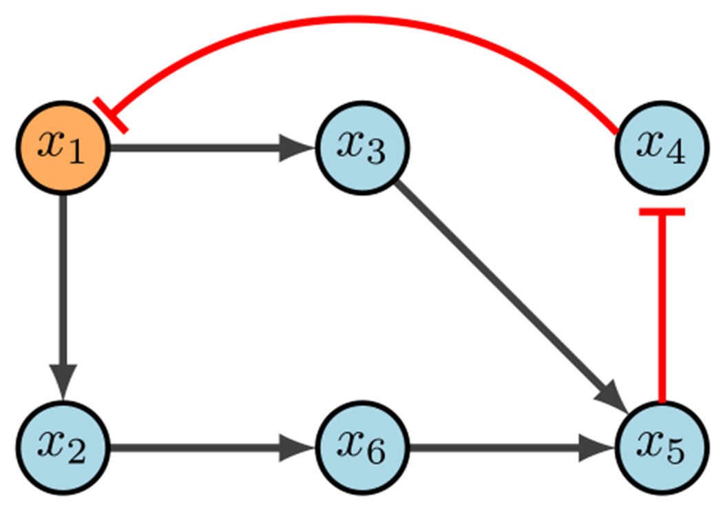
Consider the network in Fig. 14. Steady state analysis reveals two fixed points: 000100 and 111011. Suppose our control objective is $x_4=0$, which is the second fixed point respectively. We first notice that there are no input nodes, which means we move on to distinguishing nodes. Then the CK method (correctly) indicates that $x_1=1$ will direct the system into the desired fixed point. Admittedly, while the CK method is straight forward, the documentation for the software used to implement the search can be difficult to navigate (Plaugher 2022).

Fig. 15.

FVS example (Plaugher 2022)

7.2.3. Feedback Vertex Set

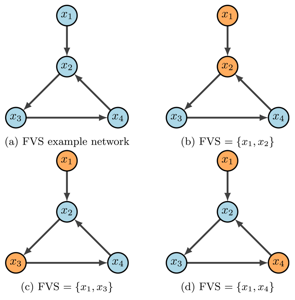
Figure 15 contains a simple example of identifying a FVS. The input node $\left(x_1\right)$ is always in the control set, while the only other node required is one of those in the 3-cycle. As scene in the figure, Fig. 15a is the example wiring diagram and Fig. 15b–d show the three possible FVS’s. One can easily see that the strategy for FVS is quite simple, yet, it can produce larger control sets than necessary. Further, we may not obtain all FVS’s if the system has many attractors (Plaugher 2022).

7.2.4. Stable Motifs

Consider the example network in Fig. 16a, with the following functions and negated functions.

$$\begin{gathered} f_1=x_2\mid x_3\sim f_1=\left(\sim x_2\right)\&\left(\sim x_3\right) \\ {f}_2=x_1\&\left(\sim x_3\right)\sim f_2=\left(\sim x_1\right)\mid x_3 \\ {f}_3=\left(\sim x_1\right)\mid \left(\sim x_2\right)\sim f_3=x_1\&x_2 \end{gathered}$$

Using the aforementioned steps, the expanded graph obtained is Fig. 16b. Notice there are two stable motifs (circled in orange and green), which indicate a fixed point (110) and a partial fixed point (X01). To find the rest of partial fixed point, substitute known values into the original functions. Therefore,

$$f_1=x_2\left|x_3=0\right|1=1$$

Fig. 16.

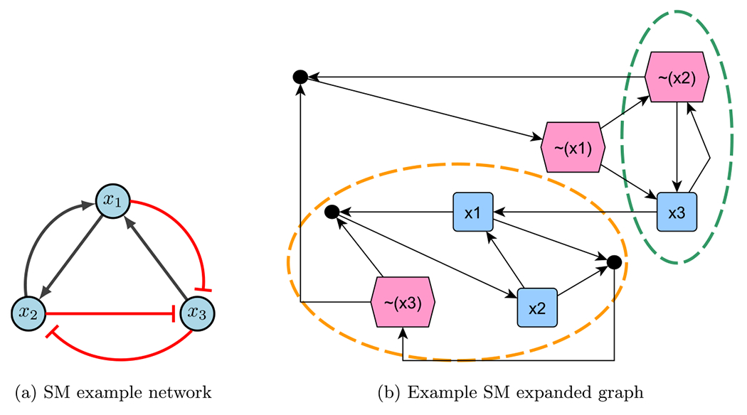
Stable motif example (Plaugher 2022)

which gives 101 as the second fixed point. Since the control sets are subsets of the stable motifs, we have $\left\{x_2=1,x_3=0\right\}$ or $\left\{x_1=1,x_3=0\right\}$ for fixed point 110, and $\left\{x_2=0\right\}$ or $\left\{x_3=1\right\}$ for fixed point 101 (Plaugher 2022).

7.3. Simulating Target Efficacy

To determine the efficacy of controls, we compare uncontrolled simulations with the appropriate target control simulations. Thus, a good control will produce low disease levels and high health levels (Plaugher 2022). We can do so by utilizing a stochastic simulator based on SDDS (Murrugarra and Aguilar 2018; Plaugher and Murrugarra 2021; Plaugher et al. 2022; Plaugher 2022), which requires several inputs before it can begin. The number of input variables in each Boolean function is given by the vector $nv$. Next, we need the variables for each gene in the form of an $m\times n$ matrix called $\mathit{var\; F}$ where $m$ is the maximum number of inputs, $n$ is the number of genes, and information is stored column-wise. The number of variables will vary between functions. Since only the first $nv(i)$ elements of the ith column are relevant, all remaining entries are set as $(-1)$. Now we construct the truth table $F$ in compact form with size $2^m\times n$. Again, the length of each column $i$ will vary but only the first $2^{nv(i)}$ entries are relevant. So all remaining entries are set as $(-1)$. It is vitally important to maintain numerical ordering, which is why the columns of $F$ are in lexicographic binary arrays (Veliz-Cuba et al. 2022).

We must also establish propensities in the form of a $2\times n$ matrix $c$ that contains values for $p_k^{\uparrow }$ and $p_k^{\downarrow }$. The values chosen for propensities may perturb results, as we saw in Fig. 12. But for all intents and purposes, we typically use $p_k^{\uparrow }=p_k^{\downarrow }=0.9$ (i.e. follow the function rules 90% of the time). Finally, we can run simulations using inputs: $F$, $\mathit{var\; F}$, $nv$, number of states (usually Boolean), $c,n$, number of steps, and number of random initializations. We have also implemented versions that allow for mutation induction and specified initial states. As a result, we achieve time-course trajectories, and we can use the Markov chain structure of SDDS to analyze features such as time to absorption, stationary distributions, and more.

Fig. 17.

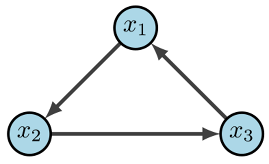
Simple 3-cycle (Plaugher 2022)

Table 6.

Variable tables for simple 3-cycle simulations in Fig. 17 (Plaugher 2022)

(a) $\mathit{nv}$
$x_2$	$x_2$	$x_3$
1	1	1
(b) $\mathit{var\; F}$
$x_1$	$x_2$	$x_3$
3	1	2
(c) $F$
$x_1$	$x_2$	$x_3$
0	0	0
1	1	1

As an example, consider the simple 3-cycle in Fig. 17. This particular system has two fixed points $(\{000\}$ and $\left\{111\right\})$ as well as two attractors $(\{001,100,010\}$ and $\{011,101,110\})$. Simulations were conducted using the variables in Table 6, with 1000 random initializations, 100 time steps (function updates), and injecting 1% noise. The overall state-space is shown in Fig. 18. In Fig. 19a, the uncontrolled simulation shows the oscillatory nature of attractors. However, Fig. 19b, c show that inducing control on $x_1$ is enough to drive the system to one fixed point or the other. Therefore, the SDDS simulator has the ability to show long-term trajectories and impact of controls over time.

7.4. Software

• Cumulative files for all control techniques and examples, as well as “how-to” documentation (Plaugher 2022)

  – https://github.com/drplaugher/SMATA_pipeline

• CA: used to find fixed points, controls, and run simulations (Plaugher and Murrugarra 2021; Plaugher et al. 2022; Grayson and Stillman 2002)

  – use the example files above

  – see also, https://github.com/drplaugher/PCC_Mutations

• CK: used to find control kernels (Borriello and Daniels 2021)

  – https://doi.org/10.5281/zenodo.5172898

• FVS: used to find FVSs (Mochizuki et al. 2013; Zañudo et al. 2017)

  – https://github.com/jgtz/FVS_python3

• Modularity: used to find strongly connected components (modules) (Kadelka et al. 2022)

  – use the example files above

• SM: used to find stable motifs and dynamic attractors (Zañudo and Albert 2015, 2013)

  – https://github.com/jgtz/StableMotifs

  – https://github.com/jcrozum/pystablemotifs

7.5. Appendix Tables

See Tables 7 and 8.

Fig. 18.

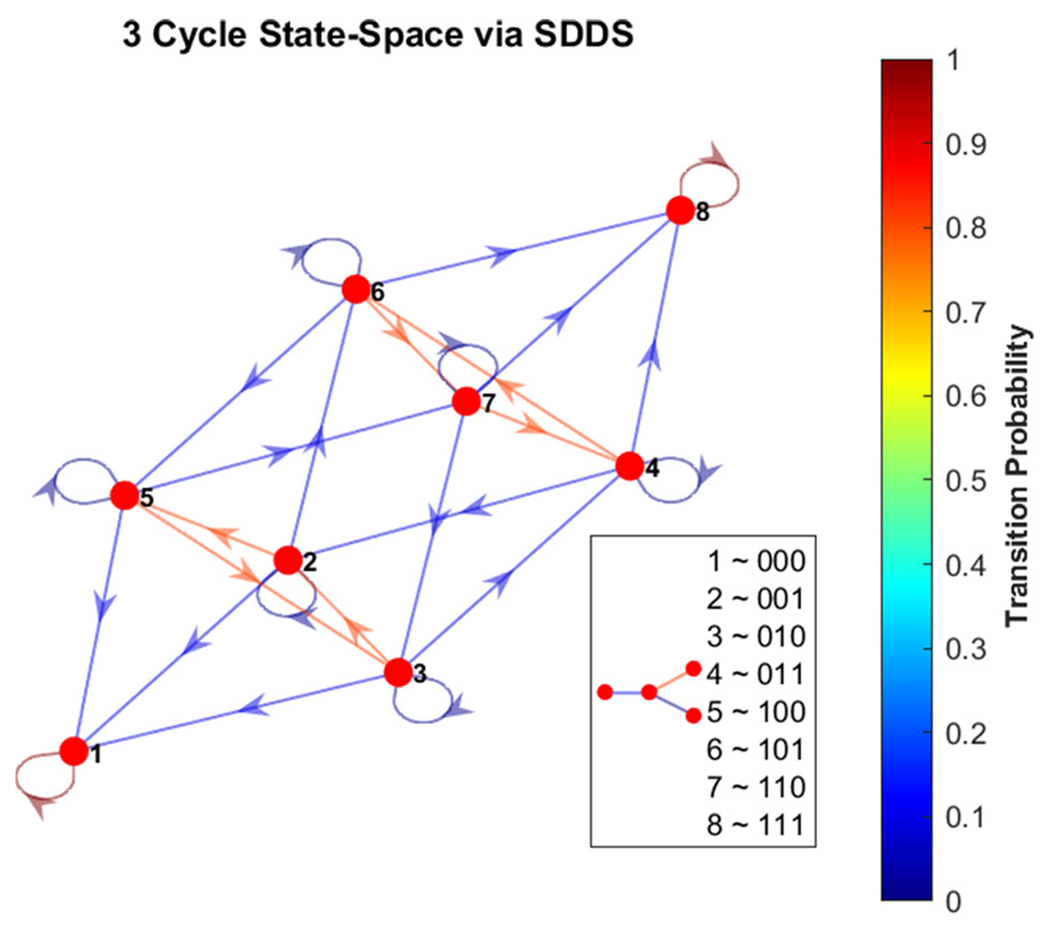
Phase-space of simple 3-cycle. Here we show the state-space of the example from Fig. 17, using SDDS with transition probabilities, with nodes written in lexicographical ordering

Fig. 19.

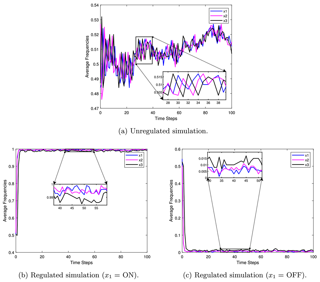
Simulation examples for a simple 3-cycle with 1% noise (Plaugher 2022)

Table 7.

Small T-LGL rules

Node	Boolean rule
S1P	(Not Ceramide)
FLIP	(Not DISC)
Fas	(Not S1P)
Ceramide	Fas and (not S1P)
DISC	Ceramide or (Fas and (not FLIP))
Apoptosis	DISC

Table 8.

Functions for large T-LGL model

Node	Rule
CTLA4	TCR
TCR	Stimuli and not CTLA4
PDGFR	S1P or PDGF
FYN	TCR or IL2RB
Cytoskeleton_signaling	FYN
LCK	CD45 or ((TCR or IL2RB) and not ZAP70)
ZAP70	LCK and not FYN
GRB2	IL2RB or ZAP70
PLCG1	GRB2 or PDGFR
KRAS	(GRB2 or PLCG1) and not GAP
GAP	(KRAS or (PDGFR and GAP)) and not (IL15 or IL2)
MEK	KRAS
ERK	MEK and PI3K
PI3K	PDGFR or KRAS
NFKB	(TPL2 or PI3K) or (FLIP and TRADD and IAP)
NFAT	PI3K
RANTES	NFKB
IL2	(NFKB or STAT3 or NFAT) and not TBET
IL2RBT	ERK and TBET
IL2RB	IL2RBT and (IL2 or IL15)
IL2RAT	IL2 and (STAT3 or NFKB)
IL2RA	(IL2 and IL2RAT) and not IL2RA
JAK	(IL2RA or IL2RB or RANTES or IFNG) and not (SOCS or CD45)
SOCS	JAK and not (IL2 or IL15)
STAT3	JAK
P27	STAT3
Proliferation	STAT3 and not P27
TBET	JAK or TBET
CREB	ERK and IFNG
IFNGT	TBET or STAT3 or NFAT
IFNG	((IL2 or IL15 or Stimuli) and IFNGT) and not (SMAD or P2)
P2	(IFNG or P2) and not Stimuli2
GZMB	(CREB and IFNG) or TBET
TPL2	TAX or (PI3K and TNF)
TNF	NFKB
TRADD	TNF and not (IAP or A20)
FasL	STAT3 or NFKB or NFAT or ERK
FasT	NFKB
Fas	(FasT and FasL) and not sFas
sFas	FasT and S1P
Ceramide	Fas and not S1P
DISC	FasT and ((Fas and IL2) or Ceramide or (Fas and not FLIP))
Caspase	(((TRADD or GZMB) and BID) and not IAP) or DISC
FLIP	(NFKB or (CREB and IFNG)) and not DISC
A20	NFKB
BID	(Caspase or GZMB) and not (BclxL or MCL1)
IAP	NFKB and not BID
BclxL	(NFKB or STAT3) and not (BID or GZMB or DISC)
MCL1	(IL2RB and STAT3 and NFKB and PI3K) and not DISC
Apoptosis	Caspase
GPCR	S1P
SMAD	GPCR
SPHK1	PDGFR
S1P	SPHK1 and not Ceramide
PDGF	0
IL15	1
Stimuli	1
Stimuli2	0
CD45	0
TAX	0

References

- Aguilar B, Gibbs DL, Reiss DJ, McConnell M, Danziger SA, Dervan A, Trotter M, Bassett D, Hershberg R, Ratushny AV, Shmulevich I (2020) A generalizable data-driven multicellular model of pancreatic ductal adenocarcinoma. Gigascience 9(7):07. [DOI] [PMC free article] [PubMed] [Google Scholar]
- Aguilar B, Fang P, Laubenbacher R, Murrugarra D (2020) A near-optimal control method for stochastic Boolean networks. Lett Biomath 7(1):67. [PMC free article] [PubMed] [Google Scholar]
- Akutsu T, Hayashida M, Ching W-K, Michael KN (2007) Control of Boolean networks: hardness results and algorithms for tree structured networks. J Theor Biol 244(4):670–679 [DOI] [PubMed] [Google Scholar]
- Arkin A, Ross J, McAdams HH (1998) Stochastic kinetic analysis of developmental pathway bifurcation in phage -infected Escherichia coli cells. Genetics 149(4):1633–1648 [DOI] [PMC free article] [PubMed] [Google Scholar]
- Baker RE, Pena J-M, Jayamohan J, Jérusalem A (2018) Mechanistic models versus machine learning, a fight worth fighting for the biological community? Biol Lett 14(5):20170660. [DOI] [PMC free article] [PubMed] [Google Scholar]
- Bender EA, Williamson SG (2010) Lists, decisions and graphs. S. Gill Williamson [Google Scholar]
- Bertsekas D (2019) Reinforcement learning and optimal control. Athena Scientific, Nashua [Google Scholar]
- Borriello E, Daniels BC (2021) The basis of easy controllability in Boolean networks. Nat Commun 12(1) [DOI] [PMC free article] [PubMed] [Google Scholar]
- Cheng D, Qi H, Li Z, Liu JB (2011) Stability and stabilization of Boolean networks. Int J Robust Nonlinear Control 21(2):134–156 [Google Scholar]
- Choo S-M, Ban B, Joo JI, Cho K-H (2018) The phenotype control kernel of a biomolecular regulatory network. BMC Syst Biol 12(1):49. [DOI] [PMC free article] [PubMed] [Google Scholar]
- Cifuentes-Fontanals L, Tonello E, Siebert H (2022) Control in Boolean networks with model checking. Front Appl Math Stat 8 [Google Scholar]
- Cifuentes-Fontanals L, Tonello E, Siebert H (2022) Node and edge control strategy identification via trap spaces in Boolean networks
- Creative Proteomics (2018) Brief introduction of post-translational modifications (PTMS). Creative Proteomics Blog [Google Scholar]
- Didier G, Remy E, Chaouiya C (2011) Mapping multivalued onto Boolean dynamics. J Theor Biol 270(1):177–184 [DOI] [PubMed] [Google Scholar]
- Erkan M, Reiser-Erkan C, Michalski C, Kleeff J (2010) Tumor microenvironment and progression of pancreatic cancer. Exp Oncol 32:128–31 [PubMed] [Google Scholar]
- Farrow B, Albo D, Berger DH (2008) The role of the tumor microenvironment in the progression of pancreatic cancer. J Surg Res 149(2):319–328 [DOI] [PubMed] [Google Scholar]
- Feig C, Gopinathan A, Neesse A, Chan DS, Cook N, Tuveson DA (2012) The pancreas cancer microenvironment. Clin Cancer Res 18(16):4266–4276 [DOI] [PMC free article] [PubMed] [Google Scholar]
- Festa P, Pardalos P, Resende M (1999) Feedback set problems. Encyclopedia of optimization 2 [Google Scholar]
- Fiedler B, Mochizuki A, Kurosawa G, Saito D (2013) Dynamics and control at feedback vertex sets. I: informative and determining nodes in regulatory networks. J Dyn Differ Equ 25(3):563–604 [Google Scholar]
- Galinier P, Lemamou E, Bouzidi M (2013) Applying local search to the feedback vertex set problem. J Heuristics 19:10 [Google Scholar]
- Gong C, Milberg O, Wang B, Vicini P, Narwal R, Roskos L, Popel AS (2017) A computational multiscale agent-based model for simulating spatio-temporal tumour immune response to pd1 and pdl1 inhibition. J R Soc Interface 14(134):20170320. [DOI] [PMC free article] [PubMed] [Google Scholar]
- Gore J, Korc M (2014) Pancreatic cancer stroma: friend or foe? Cancer Cell 25:711–712 [DOI] [PMC free article] [PubMed] [Google Scholar]
- Grayson DR, Stillman ME (2002) Macaulay2, a software system for research in algebraic geometry. http://www.math.uiuc.edu/Macaulay2/
- Heinz S, Urszula L (2016) Optimal control for mathematical models of cancer therapies: an application of geometric methods, vol 42. Springer, New York [Google Scholar]
- Hinkelmann F, Brandon M, Guang B, McNeill R, Blekherman G, Veliz-Cuba A, Laubenbacher R (2011) ADAM: analysis of discrete models of biological systems using computer algebra. BMC Bioinform 12:295. [DOI] [PMC free article] [PubMed] [Google Scholar]
- Johnson K, Plaugher D, Murrugarra D (2023) Investigating the effect of changes in model parameters on optimal control policies, time to absorption, and mixing times
- Kadelka C, Laubenbacher R, Murrugarra D, Veliz-Cuba A, Matthew W (2022) Decomposition of Boolean networks: an approach to modularity of biological systems [Google Scholar]
- Kauffman SA (1969) Metabolic stability and epigenesis in randomly constructed genetic nets. J Theor Biol 22(3):437–467 [DOI] [PubMed] [Google Scholar]
- Kleeff J, Beckhove P, Esposito I, Herzig S, Huber PE, Matthias Löhr J, Friess H (2007) Pancreatic cancer microenvironment. Int J Cancer 121(4):699–705 [DOI] [PubMed] [Google Scholar]
- Lenhart S, Workman JT (2007) Optimal control applied to biological models, 1st edn. Chapman Hall/CRC, Boca Raton [Google Scholar]
- Loughran TP (2006) Large granular lymphocytic leukemia. Leukemia and Lymphoma Society [Google Scholar]
- Macklin P (2019) Key challenges facing data-driven multicellular systems biology. Gigascience 8(10):giz127. [DOI] [PMC free article] [PubMed] [Google Scholar]
- Mochizuki A, Fiedler B, Kurosawa G, Saito D (2013) Dynamics and control at feedback vertex sets. II: a faithful monitor to determine the diversity of molecular activities in regulatory networks. J Theor Biol 335:130–146 [DOI] [PubMed] [Google Scholar]
- Moore H (2018) How to mathematically optimize drug regimens using optimal control. J Pharmacokinet Pharmacodyn 45(1):127–137 [DOI] [PMC free article] [PubMed] [Google Scholar]
- Motter AE (2015) Networkcontrology. Chaos Interdiscip J Nonlinear Sci 25(9):097621. [DOI] [PMC free article] [PubMed] [Google Scholar]
- Murrugarra D, Aguilar B (2018) Algebraic and combinatorial computational biology, chapter 5. Academic Press, New York, pp 149–150 [Google Scholar]
- Murrugarra D, Dimitrova ES (2015) Molecular network control through Boolean canalization. EURASIP J Bioinform Syst Biol 2015(1):9. [DOI] [PMC free article] [PubMed] [Google Scholar]
- Murrugarra D, Dimitrova E (2021) Quantifying the total effect of edge interventions in discrete multistate networks. Automatica 125:109453 [Google Scholar]
- Murrugarra D, Veliz-Cuba A, Aguilar B, Arat S, Laubenbacher R (2012) Modeling stochasticity and variability in gene regulatory networks. EURASIP J Bioinf Syst Biol 2012(1):5. [DOI] [PMC free article] [PubMed] [Google Scholar]
- Murrugarra D, Veliz-Cuba A, Aguilar B, Laubenbacher R (2016) Identification of control targets in Boolean molecular network models via computational algebra. BMC Syst Biol 10(1):94. [DOI] [PMC free article] [PubMed] [Google Scholar]
- Murrugarra D, Miller J, Mueller AN (2016) Estimating propensity parameters using google PageRank and genetic algorithms. Front Neurosci 10:513. [DOI] [PMC free article] [PubMed] [Google Scholar]
- Padoan A, Plebani M, Basso D (2019) Inflammation and pancreatic cancer: focus on metabolism, cytokines, and immunity. Int J Mol Sci 20:676. [DOI] [PMC free article] [PubMed] [Google Scholar]
- Plaugher D (2022) An integrated computational pipeline to construct patient-specific cancer models
- Plaugher D, Aguilar B, Murrugarra D (2022) Uncovering potential interventions for pancreatic cancer patients via mathematical modeling. J Theor Biol 548:111197. [DOI] [PubMed] [Google Scholar]
- Plaugher D, Murrugarra D (2021) Modeling the pancreatic cancer microenvironment in search of control targets. Bull Math Biol 83 [DOI] [PubMed] [Google Scholar]
- Rozum J, Albert R (2022) Leveraging network structure in nonlinear control. NPJ Syst Biol Appl 8(1):36. [DOI] [PMC free article] [PubMed] [Google Scholar]
- Saadatpour A, Albert I, Albert R (2010) Attractor analysis of asynchronous Boolean models of signal transduction networks. J Theor Biol 266(4):641–56 [DOI] [PubMed] [Google Scholar]
- Saadatpour A, Wang R-S, Liao A, Liu X, Loughran TP, Albert I, Albert R (2011) Dynamical and structural analysis of a T cell survival network identifies novel candidate therapeutic targets for large granular lymphocyte leukemia. PLoS Comput Biol 7(11):e1002267. [DOI] [PMC free article] [PubMed] [Google Scholar]
- Saadatpour A, Albert R, Reluga T (2013) A reduction method for Boolean network models proven to conserve attractors. SIAM J Appl Dyn Syst 12:1997–2011 [DOI] [PMC free article] [PubMed] [Google Scholar]
- Shmulevich I, Dougherty ER, Kim S, Zhang W (2002) Probabilistic Boolean networks: a rule-based uncertainty model for gene regulatory networks. Bioinformatics 18(2):261–274 [DOI] [PubMed] [Google Scholar]
- Shmulevich I, Dougherty ER (2010) Probabilistic Boolean networks: the modeling and control of gene regulatory networks. SIAM [Google Scholar]
- Sutton RS, Barto AG (2018) Reinforcement learning: an introduction. MIT Press, Cambridge [Google Scholar]
- Taylor BP, Dushoff J, Weitz JS (2016) Stochasticity and the limits to confidence when estimating r0 of Ebola and other emerging infectious diseases. J Theor Biol 408:145–154 [DOI] [PubMed] [Google Scholar]
- Thomas R (1973) Boolean formalization of genetic control circuits. J Theor Biol 42(3):563–585 [DOI] [PubMed] [Google Scholar]
- Veliz-Cuba A (2011) Reduction of Boolean network models. J Theor Biol 289:167–172 [DOI] [PubMed] [Google Scholar]
- Veliz-Cuba A, Aguilar B, Hinkelmann F, Laubenbacher R (2014) Steady state analysis of Boolean molecular network models via model reduction and computational algebra. BMC Bioinform 15:221. [DOI] [PMC free article] [PubMed] [Google Scholar]
- Veliz-Cuba A, Voss SR, Murrugarra D (2022) Building model prototypes from time-course data. Lett Biomath 9(1):107–120 [Google Scholar]
- Vieira LS, Laubenbacher RC, Murrugarra D (2020) Control of intracellular molecular networks using algebraic methods. Bull Math Biol 82(1):1–22 [DOI] [PMC free article] [PubMed] [Google Scholar]
- Waddington CH (1957) The strategy of the genes: a discussion of some aspects of theoretical biology. Allen & Unwin, London [Google Scholar]
- Yang J-M, Lee C-K, Cho K-H (2020) Stabilizing control of complex biological networks based on attractor-specific network reduction. IEEE Trans Control Netw Syst 8(2):928–939 [DOI] [PubMed] [Google Scholar]
- Yang J-M, Lee C-K, Cho K-H (2021) Stabilizing control of complex biological networks based on attractor-specific network reduction. IEEE Trans Control Netw Syst 8(2):928–939 [DOI] [PubMed] [Google Scholar]
- Yang G, Zañudo JGT, Albert R (2018) Target control in logical models using the domain of influence of nodes. Front Physiol 9 [DOI] [PMC free article] [PubMed] [Google Scholar]
- Yousefi MR, Datta A, Dougherty ER (2012) Optimal intervention strategies for therapeutic methods with fixed-length duration of drug effectiveness. IEEE Trans Signal Process 60(9):4930–4944 [Google Scholar]
- Zañudo J, Albert R (2013) An effective network reduction approach to find the dynamical repertoire of discrete dynamic networks. Chaos (Woodbury, NY) 23:025111. [DOI] [PubMed] [Google Scholar]
- Zañudo JGT, Albert R (2015) Cell fate reprogramming by control of intracellular network dynamics. PLoS Comput Biol 11(4):e1004193. [DOI] [PMC free article] [PubMed] [Google Scholar]
- Zañudo JGT, Yang G, Albert R (2017) Structure-based control of complex networks with nonlinear dynamics. Proc Natl Acad Sci USA 114(28):7234–7239 [DOI] [PMC free article] [PubMed] [Google Scholar]