

Abstract
Background
Obtaining accurate drug–target binding affinity (DTA) information is significant for drug discovery and drug repositioning. Although some methods have been proposed for predicting DTA, the features of proteins and drugs still need to be further analyzed. Recently, deep learning has been successfully used in many fields. Hence, designing a more effective deep learning method for predicting DTA remains attractive.
Results
Dynamic graph DTA (DGDTA), which uses a dynamic graph attention network combined with a bidirectional long short-term memory (Bi-LSTM) network to predict DTA is proposed in this paper. DGDTA adopts drug compound as input according to its corresponding simplified molecular input line entry system (SMILES) and protein amino acid sequence. First, each drug is considered a graph of interactions between atoms and edges, and dynamic attention scores are used to consider which atoms and edges in the drug are most important for predicting DTA. Then, Bi-LSTM is used to better extract the contextual information features of protein amino acid sequences. Finally, after combining the obtained drug and protein feature vectors, the DTA is predicted by a fully connected layer. The source code is available from GitHub at https://github.com/luojunwei/DGDTA.
Conclusions
The experimental results show that DGDTA can predict DTA more accurately than some other methods.
Keywords: Drug–target binding affinity, Dynamic graph attention network, Long short-term memory, Drug discovery
Background
Drug–target interaction (DTI) prediction is a critical task in drug discovery and drug repositioning [1, 2]. Structural changes to a drug can significantly alter its binding affinity with proteins [3], making it important to predict whether a drug can bind to a specific protein. However, the traditional high-throughput screening experiments used to detect this activity are expensive and time-consuming [4]. Therefore, computing methods for DTI prediction have become popular and effective [5, 6].
DTI calculation methods focus on binary classification [2, 7], and the main goal is to determine whether a drug and a target interact with each other [8]. However, the assumed binding strength values of the given protein and the drug compound are continuous and referred to as their binding affinity. The drug–target pair prediction task is described as an affinity prediction problem [8] in which, the binding affinity score is directly used, thus creating a more realistic experiment. In addition, regression-based models are more advantageous in approximating the strength of DTIs [9], making them more conducive to the discovery of new drug compounds in the limited drug research space.
Recently, some methods [10, 11] for predicting drug–target affinity (DTA) have been developed. SimBoost [11] enhances the performance of learning-based methods by extracting features from drugs, targets, and drug–target pairs and providing them to gradient-enhanced supervised learning methods. Affinity is characterized by an inhibition constant (), dissociation constant (), changes in free energy measures (,), half-maximal inhibition constant () [12], half-maximal activity concentration () [13], KIBA score [14] and scoring. Stronger affinity readings indicate greater DTIs [15]. In the KronRLS [10, 16] model, the Kronecker products of a drug and target are constructed by drug and protein pairs to calculate the kernel K of the pairs, which is entered into a regularized least-squares regression model (RLS) to predict the binding affinity.
With the success of deep learning, various deep networks have been used for DTA prediction [8, 13], and have achieved better performance than machine learning. Some prediction methods are summarized in Table 1. In the DeepDTA [8] model, one-dimensional sequences of drugs and proteins are fed into a convolutional neural network (CNN) to extract the features of drugs and their targets through the (simplified molecular input line entry system) SMILES string representations of the drugs, and good results have been achieved. The PADME [13] model combines molecular graph convolution of compounds and protein features and uses fixed-rule descriptors to represent proteins, improving the predictive performance of the model. The model is more scalable than traditional machine learning models. WideDTA [17] builds on DeepDTA [8] by representing drugs and proteins as words, learning more potential characteristics of drugs and proteins. However, since the convolution window of a CNN is fixed, this network is unable to extract the features of contextual information. To represent molecules in a natural way that preserves as much molecular structure information as possible, thus allowing the model to better learn the relevance of the underlying space, an increasing number of approaches are utilizing graph neural networks to predict DTA. MT-DTI [18] introduces the attention mechanism in drug representation and takes more account of the correlation between different molecules, which improves the prediction performance of DTA and greatly increases the interpretability. In DeepGS [19], the topological structure information of a drug is extracted by using a graph attention network (GAT) [20], while the local chemical background of the drug is captured by using a bidirectional gated recurrent unit (Bi-GRU) [21] and combined with the protein sequence features extracted by a CNN for prediction. rzMLP [22] uses a gMLP model to aggregate input features with constant size, and uses a ReZero layer to smooth the training process for that block. The model is able to learn more complex global features while avoiding poor predictions due to a too deep model. EnsembleDLM [23] aggregates predictions from multiple deep neural networks, not only obtaining better predictions, but also exploring how much data deep learning networks need to achieve better prediction performance. GANsDTA [24] employs a generative adversarial network (GAN) [25] to extract features of protein sequences and compound SMILES in an unsupervised manner. Because GAN’s feature extractor does not require labeled data, the model is able to accommodate unlabeled data for training. Because GAN’s feature extractor does not require labeled data, the model is able to accommodate unlabeled data for training. The model can use more datasets to learn protein and drug features, thus achieving correspondingly better feature representation and prediction performance. GraphDTA [26] modelled drugs as molecular graphs with one-dimensional drug sequences, then put the graph into several graph network models and obtained deep learning models, which were excellent at the time. GraphDTA [26] demonstrated that representing drugs as graphs can further improve the prediction capabilities of deep learning models in terms of DTA.
Table 1.
Prediction methods
| Method | Published time | Model | Summary |
|---|---|---|---|
| SimBoost [11] | 2016 | Gradient boosting regression trees | Predicting continuous values of binding affinities of compounds and proteins |
| KronRLS [16] | 2018 | Multiple kernel learning | The first method for time- and memory-efficient learning with multiple pairwise kernels |
| DeepDTA [8] | 2018 | CNN | Processing protein sequences and compound 1D representations using convolutional neural networks |
| PADME [13] | 2018 | DNN | The first to combine Molecular Graph Convolution for compound featurization with protein descriptors |
| WideDTA [17] | 2019 | CNN | Combining four different textual pieces of information related to proteins and ligands |
| MT-DTI [18] | 2019 | Transformers + CNN | Proposing a new molecule representation based on the self-attention mechanism |
| GANsDTA [24] | 2019 | GAN + CNN | Effectively learning valuable features from labeled and unlabeled data |
| DeepGS [19] | 2020 | GAT + Bi-GRU | Extracting the topological information of the molecular map and the local chemical context of the drug |
| rzMLP [22] | 2021 | gMLP + ReZero | Use MHM block for multiple protein and ligand representations and rzMLP block to aggregate concatenated protein-ligand pair representations |
| EnsembelDLM [23] | 2021 | Multiple deep networks | Aggregating predictions from multiple deep neural networks |
| GraphDTA [26] | 2021 | GIN + CNN | Introducing multiple models of graph neural networks |
However, two problems remain that prevent accurate DTA. (1) The GAT model used by some contemporary methods is a restricted form of static attention, and the attention coefficient function of the nodes in the drug graph is monotonic, which leads to the inability to comprehensively extract drug features. (2) When processing protein sequences, the contextual association information of amino acid sequences is not acquired, and the protein association features are thus ignored.
To solve the above problem, this paper proposes a method named dynamic graph DTA (DGDTA). In DGDTA, each drug is considered a graph of interactions between atoms and edges, and a dynamic attention score is used to consider which atoms and edges in the drug graph play more critical roles in predicting DTA. Compared with static attention, DGDTA is able to extract a more comprehensive drug signature. To better obtain the contextual features of amino acid sequences in proteins, DGDTA introduces bidirectional long short-term memory (Bi-LSTM) [27] to extract more comprehensive amino acid sequence features in combination with drugs. Through validations conducted on the Davis [28] and KIBA [14] datasets, DGDTA achieves better performance than the competing methods in terms of results. In this paper, a dynamic graph attention network example is given to further improve the representativeness and effectiveness of drug molecule maps. The experimental results demonstrate the effectiveness of DGDTA.
Methods
DGDTA is a method for predicting DTA based on a deep learning network, and its architecture (shown in Fig. 1), is divided into three main steps. (1) Obtaining drug features. DGDTA uses the SMILES [29] as the drug compound input, and transforms the drug into a drug graph consisting of atoms and edges with reference to the natural properties of the drug. According to the literature, a two-layer graph network structure has better feature extraction performance. DGDTA uses a two-layer dynamic graph attention network (GATv2) [30] and a combination of GATv2 and a graph convolutional network (GCN) to obtain drug graph features, and DGDTA is divided into two versions: DGDTA-AL and DGDTA-CL. (2) Extracting protein features. DGDTA uses a combination of Bi-LSTM and multilayer convolutional networks to obtain more comprehensive protein amino acid sequence information while considering the contextual relationships among the amino acid sequences. (3) Performing DTA prediction. The observed connections among drug features and protein features during extraction used to determine DTA via a fully connected layer. The details of DGDTA are described in the following parts.
Fig. 1.

General architecture of DGDTA
Obtaining drug features
With the development of graph neural networks for DTA, many approaches have been presented. When using a graph to represent a drug, it is difficult to accurately extract graph features due to the complexity of drug graphs. DGDTA adopts a dynamic GAT to obtain drug features. Through SMILE code, drug’s atomic composition, and the valence charge number of atoms can be inferred, which can further judge drug information such as the number of hydrogen bonds, and then used for the drug’s feature representation in affinity prediction. To better extract drug features, DGDTA uses the SMILES [29] sequences of drugs as inputs, and uses RDKit to extract the atoms and interactions from the SMILES sequences. Then, DGDTA constructs a graph for each drug based on its SMILES sequence. A drug graph is denoted as , where is a node represented by a drug atom, and represents the set of edges between nodes. Each node is represented by an n-dimensional vector from DeepChem [31]. This n-dimensional vector includes the atomic symbols, the number of adjacent hydrogen atoms, the number of adjacent atoms, the implicit valence of the atoms (implicit valence) and whether the bonds are aromatic. One node is represented as . By representing the atoms d of each drug as the vertices of the drug graph, the features of each drug are obtained. To obtain more information about the graph structure in n-dimensional space, this paper adopts a dynamic attention mechanism for the graph:
| 1 |
denotes the importance of the features of neighbour node to node , where represents the neighbours of node , , are learned, and II denotes vector concatenation. Utilizing the function to normalize all neighbours, we can obtain the following attention function:
| 2 |
Combining Eqs. (1) and (2), the coefficients of attention are expressed as:
| 3 |
After integrating the feature information of the neighbouring nodes, we apply the nonlinear parameter , to obtain the output features of each node:
| 4 |
Nodes are represented as the weighted averages of their neighbouring feature vectors. To further solidify the learning process of dynamic graph self-attention and improve the learning effect, the attention is extended to multiheaded attention.
| 5 |
independent attention mechanisms connect the semantic feature vectors of the nodes through Eq. (5), and obtain an updated drug feature representation . Based on a combination of research and experiments, a two-layer graph network structure is able to obtain more accurate prediction results. First, the graph network in the second layer uses a dynamic graph neural network and obtains the drug feature representations ; this version is named DGDTA-AL. After many experiments and comparisons, the graph network in the second layer is replaced with a GCN, whose propagation rules are as follows:
| 6 |
denotes the nodal feature matrix of , where , is the adjacency matrix, is the unit matrix, , is the degree matrix, and is a trainable weight. A drug feature representation is obtained. The GCN is applied to the full graph via the Laplacian matrix, which captures the connectivity relationships between the graph nodes and updates the node features of the full graph. In this paper, this version is named DGDTA-CL. We use the rectified linear unit () activation function after each layer and use global maximum pooling in the last layer to obtain the vector representation of the drug.
Extracting protein features
A protein sequence is a string of ASCII characters represented as amino acids. In many methods, one-hot codes are used to represent drugs and proteins, as well as other biological sequences, such as DNA and RNA. We use one-hot encoding to represent the atoms of the drug and incorporate atomic properties for drug initialization. Because drug molecules are shorter and simpler in structure than proteins, we utilize one-hot encoding to expand the dimensionality of the drug’s representation. This enables model to capture specific information associated with each drug atom. For protein, in order to prevent feature singularity, we employ different approaches for the initialization. In this paper, we map each amino acid to a numerical value and represent one protein as a sequence of integers. And then an embedding layer is added to the sequence, where each character is represented by a 128-dimensional vector. For training purposes, the sequences are cut or padded to a fixed sequence with a length of 1000. If the sequence is short, it is padded with 0 values. In this paper, the embedding representation (, where is the dimensionality of the protein embedding) is a Bi-LSTM layer that captures the dependencies the characters in a sequence of length (). We obtain , where denotes the number of output cells used in each LSTM cell.
| 7 |
| 8 |
| 9 |
The vector is composed of the output vectors generated by the Bi-LSTM; i.e., . Finally, we use a one-dimensional convolutional layer to learn different levels of abstract features to obtain a vector of protein sequences representations.
Performing DTA prediction
The prediction layer connects the learned drug vector representation with the vector representation of the protein sequence. Then, they are used as inputs and the output is obtained from the fully connected layer.
| 10 |
where denotes the weight matrix of the fully connected layer and denotes the bias of the fully connected layer.
We choose the mean square error (MSE) loss as the loss function, which has the advantage of a function curve that is smooth, continuous and derivable everywhere, making it convenient for use in the gradient descent algorithm. As the error decreases, the gradient also decreases, which is more conducive to convergence and more stable.
| 11 |
where , denotes the predicted affinity value between the th sample and the label of the affinity value in the sample, and denotes the batch size.
Model training
DGDTA takes drug SMILES strings and protein amino acid sequences as inputs. In this paper, Python 3.9, PyTorch 1.12.1 and PyG2.1 are used to implement dynamic GAT and LSTM. In this paper, the number of layers in the graph neural network is set to 2, Bi-LSTM is applied, the number of hidden states is set to 10, and the dropout parameter is set to 0.2. Then, the proposed method is trained on the above dataset for 1000 epochs, and the adaptive moment estimation (Adam) optimizer is used with a learning rate of 0.0005. The devices that are used for the experiments are an Intel(R) Xeon(R) Platinum 8260 CPU @ 2.30 GHz and an NVIDIA GeForce RTX 3090 GPU.
Results
In this section, we present the dataset used, the evaluation metrics, an ablation study and the results of a comparison with state-of-the-art methods. This section also illustrates the advantage of the dynamic GAT and gives an example of a real drug–target combination.
Dataset and evaluation metrics
We use the Davis [28] and KIBA [14] datasets to evaluate the performance of the method proposed in this paper. The numbers of drugs and targets in the dataset, and the sample sizes for training and testing during the experiments are shown in Table 2. In this paper, the concordance index (CI; the larger the better) [32] and MSE (the smaller the better) are also used as the main indicators for evaluating the performance of the tested models. In this paper, the GAT and GAT_GCN models are chosen as baseline1 and baseline2 of the ablation study, respectively.
Table 2.
Datasets
| Davis | KIBA | |
|---|---|---|
| Drugs | 72 | 2116 |
| Targets | 442 | 229 |
| Total samples | 30,056 | 118,254 |
| Train samples | 25,046 | 98,545 |
| Test samples | 5010 | 19,709 |
Ablation study
In the ablation study, we analyse the effectiveness of the innovative elements of our method. In this section, to be as fair as possible, we use the same training and testing sets as those employed by the baselines and the same evaluation metrics. In this paper, a dynamic graph neural network is incorporated into the drug graph, and Bi-LSTM is added to extract protein amino acid sequence features to further improve the model accuracy. The popular GRU model is added as a comparison method. GRU and LSTM are important variants of recurrent neural networks, and they have strong memory and long-distance dependence capturing ability when processing sequence data. GRU has higher computational efficiency with reduced parameter settings compared to LSTM, but this also leads to some loss of information at longer distances in some cases. In order to better capture the contextual association information of amino acid sequences and further prove the effectiveness of LSTM method, GRU is introduced as a comparison in the ablation study. And the results of the ablation study are shown in Figs. 2 and 3.
Fig. 2.

Comparison between baseline1 and different models at 200 and 1000 epochs
Fig. 3.

Comparison between baseline2 and different models at 200 and 1000 epochs
Figure 2 shows that on the Davis and KIBA datasets, the DTA prediction results obtained by Model-2 using the dynamic GAT achieve a higher CI and a smaller MSE than those of baseline 1 in the same number of epochs. Model-1 with the addition of Bi-LSTM method is also better than baseline1. Based on Model-2, Bi-LSTM is used to improve the ability to extract contextual protein amino acid sequence features. The evaluation score of Model-4 is improved further, while the prediction result is better than that of the GRU in Model-3 with the same parameters. Model-4 achieves the best results in the 200-epoch and 1000-epoch comparisons conducted on both datasets, and Model-4 is the DGDTA-AL method illustrated in 2.1. As shown in Fig. 3, Model-8 obtains the highest CI and the lowest MSE in the comparison with baseline 2 over the same number of epochs; Model-8 is the DGDTA-CL method.
In this paper, the results obtained by different models in the ablation study are presented in Table 3. On the Davis dataset, DGDTA-AL achieves the best results (in bold), reaching 0.899 and 0.225 CI and MSE values, respectively, which are improvements of 0.7% and 0.7% over those of baseline. DGDTA-CL achieves a CI of 0.902 and an MSE of 0.125 on the KIBA dataset, which are improvements of 1.1% and 1.4% over those of baseline 2, respectively. The results of the ablation study demonstrate the effectiveness of the innovative elements proposed in this paper.
Table 3.
Ablation study on the Davis and KIBA datasets
| Dataset | Methods | GATv2 | GCN | GRU | LSTM | CI | MSE |
|---|---|---|---|---|---|---|---|
| Davis | Baseline1 | – | – | – | – | 0.892 | 0.232 |
| Model-1 | – | – | – | ✓ | 0.893 | 0.230 | |
| Model-2 | ✓ | – | – | – | 0.895 | 0.232 | |
| Model-3 | ✓ | – | ✓ | – | 0.896 | 0.228 | |
| Model-4 | ✓ | – | – | ✓ | 0.899* | 0.225 | |
| Baseline2 | – | ✓ | – | – | 0.881 | 0.245 | |
| Model-5 | – | ✓ | – | ✓ | 0.886 | 0.241 | |
| Model-6 | ✓ | ✓ | – | – | 0.883 | 0.242 | |
| Model-7 | ✓ | ✓ | ✓ | – | 0.887 | 0.239 | |
| Model-8 | ✓ | ✓ | – | ✓ | 0.889 | 0.237 | |
| KIBA | Baseline1 | – | – | – | – | 0.866 | 0.179 |
| Model-1 | – | – | – | ✓ | 0.867 | 0.172 | |
| Model-2 | ✓ | – | – | – | 0.869 | 0.175 | |
| Model-3 | ✓ | – | ✓ | 0.871 | 0.169 | ||
| Model-4 | ✓ | – | – | ✓ | 0.878 | 0.162 | |
| Baseline2 | – | ✓ | – | – | 0.891 | 0.139 | |
| Model-5 | ✓ | – | ✓ | 0.896 | 0.131 | ||
| Model-6 | ✓ | ✓ | – | – | 0.893 | 0.135 | |
| Model-7 | ✓ | ✓ | ✓ | – | 0.898 | 0.128 | |
| Model-8 | ✓ | ✓ | – | ✓ | 0.902 | 0.125 |
*Bold values represent the best result
Comparison with the state-of-the-art methods
In this section, Table 4 shows the experimental results obtained by DGDTA and the comparison methods. To be consistent with the ablation experiment in 3.2, we use the same datasets and evaluation metrics. Based on this, we added the evaluation metric. As shown in Table 4, DGDTA-AL is better than the mainstream DTA methods in terms of the CI, MSE and on the Davis dataset. Compared with DeepGLSTM [33], which has the best results among the comparison methods, the CI and MSE of the proposed approach are improved by 0.6% and 1.1%, respectively. Additionally, the CI and MSE are improved by 0.9% and 0.4%, respectively, over those of the excellent MATT-DTI [34] method. And, reaches 0.707. As shown in Table 4, DGDTA-CL achieves a more significant improvement in its results on the KIBA dataset. Compared with the DeepGLSTM [33] method, DGDTA-CL attains 1.2% and 1.8% performance improvements in terms of the CI and MSE metrics, and 1.3% and 2.5% CI and MSE improvements are achieved over the MATT-DTI [34] method, respectively. And, reaches 0.809. Figure 4 plots the CI scores obtained by the methods in the table for both datasets to further demonstrate the performance improvement provided by the DGDTA method. The experimental results show that DGDTA is better than the comparative methods, and the use of a dynamic graph with attention to extract drug features and effective contextual protein information is significant for predicting DTA.
Table 4.
Comparison with the state-of-the-art methods
| Dataset | Methods | CI | MSE | |
|---|---|---|---|---|
| Davis | DeepDTA [8] | 0.878 | 0.261 | 0.631 |
| DeepCDA [35] | 0.891 | 0.248 | 0.652 | |
| MATT-DTI [34] | 0.890 | 0.229 | 0.688 | |
| GraphDTA(GAT) [26] | 0.892 | 0.232 | 0.689 | |
| GraphDTA(GAT-GCN) [26] | 0.881 | 0.245 | 0.667 | |
| CPInformer [6] | 0.874 | 0.277 | 0.621 | |
| DeepGLSTM [33] | 0.893 | 0.236 | 0.679 | |
| DGDTA-CL (ours) | 0.889 | 0.237 | 0.672 | |
| DGDTA-AL (ours) | 0.899* | 0.225 | 0.707 | |
| KIBA | DeepDTA [8] | 0.863 | 0.194 | 0.673 |
| DeepCDA [35] | 0.889 | 0.176 | 0.682 | |
| MATT-DTI [34] | 0.889 | 0.150 | 0.762 | |
| GraphDTA(GAT) [26] | 0.866 | 0.179 | 0.738 | |
| GraphDTA(GAT-GCN) [26] | 0.891 | 0.139 | 0.789 | |
| CPInformer [6] | 0.867 | 0.183 | 0.678 | |
| DeepGLSTM [33] | 0.890 | 0.143 | 0.789 | |
| DGDTA-AL (ours) | 0.881 | 0.162 | 0.762 | |
| DGDTA-CL (ours) | 0.902 | 0.125 | 0.809 |
*Bold values represent the best result
Fig. 4.

CI comparison among the experimental methods on the Davis and KIBA datasets
Advantages of the DGDTA model
A dynamic GAT suggests that a traditional GAT is only a computationally constrained form of “static” attention: for any query node, the attention function is monotonic with respect to the key fraction [30]. As shown in the GAT heatmap presented in Fig. 5, the ordering of the attention coefficients is global, and all queries focus primarily on the 7th key.
| 12 |
Fig. 5.

Attention coefficients of the GAT and GATv2
Formula (10) is the method for calculating the attention coefficients in the GAT, indicating the importance of the feature of node to node . As is limited, there exists node where the attention distribution only calculates static attention from due to it being the maximum value. To overcome the monotonicity restriction of the key score, Formula (12) is transformed into Formula (1). This variant is more expressive than the GAT, as shown in the attention maps of GATv2 in Fig. 5. Since static attention cannot have different correlations for different keys and different queries, if there is one key that has a higher attention score than the others, then no query can ignore the score of this key, which results in very limited static attention.
Among the datasets, Davis contains 2457 positive samples and 27,599 negative samples, the total number of samples is small, and the label distribution in the dataset is unbalanced. KIBA has 22,729 positive samples and 95,525 negative samples, so it contains more samples than Davis, but most of the labels in KIBA are very concentrated, and the label distribution is relatively normal. These problems create barriers for the model in terms of affinity prediction. Dynamic graph attention pays different amounts of attention to different queries in the attention score, enabling it to better distinguish the similarities and differences between samples. It is more discriminative during drug graph extraction and alleviates the imbalance problem in the given dataset. Figure 6 shows the MSE changes exhibited by the DGDTA-AL, DGDTA-CL, baseline 1 and baseline 2 models on Davis and KIBA at 200 and 500 epochs. Blue and green represent our proposed models with faster decreasing trends. The results demonstrate the more significant improvement yielded by the dynamic GAT in terms of predicting DTA.
Fig. 6.
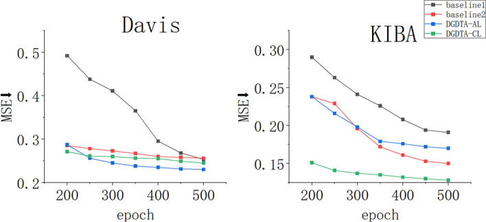
MSE trend
Example of a realistic drug–target combination
To further demonstrate the validity of the proposed method, this paper gives an example to show the 3D model produced for a tested sample in reality. As shown in Fig. 7, the targeted drug (sunitinib) inhibits receptor tyrosine kinases (RTKs), where certain receptor tyrosine kinases are involved in tumour growth, pathological blood vessel formation and tumour metastasis. In biological and cytometric assays, sunitinib has been shown to inhibit tumour growth, cause tumour regression and inhibit tumour metastasis. In this paper, the bound small drug molecules are scaled up on the right side, and the drug and its binding target correspond to the drug ‘DB5329102’ and the target ‘ITK’ in the test set, respectively; this is done to verify the validity and practicality of the model proposed in this paper in practical applications through known drug–target binding examples.
Fig. 7.
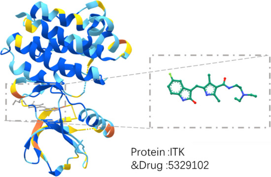
Visualization of the binding of a drug ‘DB5329102’ and a target ‘ITK’
Discussion
In this paper, DGDTA is proposed based on the dynamic graph attention model and is divided into two versions, DGDTA-AL and DGDTA-CL, to predict the affinity values between drugs and proteins. Ablation experiments are performed on the Davis and KIBA datasets, and the proposed approach is compared with the DTA models that are popular today. The experimental results show that DGDTA can achieve better prediction performance and demonstrate that the dynamic graph attention model can extract more comprehensive feature representations from molecular drug maps.
Conclusions
DGDTA can effectively predict DTA via deep learning, and it can obtain high CI and MSE metrics on experimental datasets, but it still has shortcomings. First, while dynamic graph attention models attain good prediction performance, they also require increased prediction time and computational cost. Second, drugs and proteins have very complex spatial structures, and much characteristic drug and protein information is lost in one-dimensional sequences.
In the future, further consideration will be given to fusing other characteristic drug information, such as their side effects, physicochemical properties, and deep structures. This will contribute to improving the performance of drug–target binding prediction models from various aspects.
Acknowledgements
Not applicable.
Abbreviations
- DGDTA
Dynamic graph DTA
- DTA
Drug–target binding affinity
- GAT
Graph attention network
- Bi-LSTM
Bidirectional long short-term memory
- SMILES
Simplified molecular input line entry system
- CNN
Convolutional neural network
- Bi-GRU
Bidirectional gated recurrent unit
- GAN
Generative adversarial network
- GATv2
Dynamic graph attention network
- RTK
Receptor tyrosine kinases
- GCN
Graph convolutional network
Author contributions
HZ, HH and JL participated in the design of the study and the analysis of the experimental results. HH and XL performed the implementation, prepared the tables and figures, and summarized the results of the study. ZW and JW checked the format of the manuscript. All authors have read and approved the final manuscript for publication.
Funding
The authors declare that they have no competing interests. This work has been supported in part by the National Natural Science Foundation of China under Grant No. 61972134, Young Elite Teachers in Henan Province No. 2020GGJS050, Doctor Foundation of Henan Polytechnic University under Grant No. B2018-36, Innovative and Scientific Research Team of Henan Polytechnic University under No. T2021-3, Innovation Project of New Generation Information Technology under No. 2021ITA09021.
Availability of data and materials
The Davis and KIBA data can be downloaded from https://github.com/thinng/GraphDTA/tree/master. The software and sample result as part of this project are readily avail- able from GitHub at https://github.com/luojunwei/DGDTA. Project name: DGDTA. Project home page: https://github.com/luojunwei/DGDTA. Operating system(s): Linux or other unix-like systems. Programming language: python 3.x. License: GNU GPL v3. Any restrictions to use by non-academics: license needed.
Declarations
Ethics approval and consent to participate
Not applicable.
Consent for publication
Not applicable.
Competing interests
The authors declare no competing interests.
Footnotes
Publisher’s Note
Springer Nature remains neutral with regard to jurisdictional claims in published maps and institutional affiliations.
References
- 1.Strittmatter SM. Old drugs learn new tricks. Nat Med. 2014;20(6):590. doi: 10.1038/nm.3595. [DOI] [PMC free article] [PubMed] [Google Scholar]
- 2.Affinity2Vec drug–target binding affinity prediction through representation learning, graph mining, and machine learning. Sci Rep. 2022;12(1):1–18. doi: 10.1038/s41598-022-08787-9. [DOI] [PMC free article] [PubMed] [Google Scholar]
- 3.Wan S, Kumar D, Ilyin V, Homsi UA, Coveney PV. The effect of protein mutations on drug binding suggests ensuing personalised drug selection. Sci Rep. 2021;11(1):13452. doi: 10.1038/s41598-021-92785-w. [DOI] [PMC free article] [PubMed] [Google Scholar]
- 4.Ashburn TT, Thor KB. Drug repositioning: identifying and developing new uses for existing drugs. Nat Rev Drug Discov. 2004;3(8):673–683. doi: 10.1038/nrd1468. [DOI] [PubMed] [Google Scholar]
- 5.Guan J, Tian K, Wang Y, Shao M, Zhou S. Boosting compound-protein interaction prediction by deep learning. Methods Companion Methods Enzymol. 2016;110:64–72. doi: 10.1016/j.ymeth.2016.06.024. [DOI] [PubMed] [Google Scholar]
- 6.Hua Y, Song X, Feng Z, Wu XJ, Kittler J, Yu DJ. CPInformer for efficient and robust compound–protein interaction prediction. IEEE/ACM Trans Comput Biol Bioinform. 2022;20:285–296. doi: 10.1109/TCBB.2022.3144008. [DOI] [PubMed] [Google Scholar]
- 7.Thomas KL. Predicting new molecular targets for known drugs. Nature. 2009;462(7270):175–81. doi: 10.1038/nature08506. [DOI] [PMC free article] [PubMed] [Google Scholar]
- 8.Hakime Z, Arzucan Z, Elif O. DeepDTA: deep drug–target binding affinity prediction. Bioinformatics. 2018;34(17):i821–i829. doi: 10.1093/bioinformatics/bty593. [DOI] [PMC free article] [PubMed] [Google Scholar]
- 9.Krisztian B, Ladislav P, Júlia K. Modified linear regression predicts drug–target interactions accurately. PLoS ONE. 2020;15(4):e0230726. doi: 10.1371/journal.pone.0230726. [DOI] [PMC free article] [PubMed] [Google Scholar]
- 10.Cichonska A, Ravikumar B, Parri E, Timonen S, Pahikkala T, Airola A, Wennerberg K, Rousu J, Aittokallio T. Computational-experimental approach to drug–target interaction mapping: a case study on kinase inhibitors. PLoS Comput Biol. 2017;13(8):e1005678. doi: 10.1371/journal.pcbi.1005678. [DOI] [PMC free article] [PubMed] [Google Scholar]
- 11.He T. SimBoost: a read-across approach for drug–target interaction prediction using gradient boosting machines. J. Cheminform. 2016;9:1–14. doi: 10.1186/s13321-017-0209-z. [DOI] [PMC free article] [PubMed] [Google Scholar]
- 12.Wang YB, Yi HC, Yang S, Chen ZH, Zheng K. A deep learning-based method for drug–target interaction prediction based on long short-term memory neural network. BMC Med Inf Decis Mak. 2020;20(Suppl 2):49. doi: 10.1186/s12911-020-1052-0. [DOI] [PMC free article] [PubMed] [Google Scholar]
- 13.Feng Q, Dueva E, Cherkasov A, Ester M. PADME: a deep learning-based framework for drug–target interaction prediction. 2018.
- 14.Tang J, Szwajda A, Shakyawar S, Xu T, Aittokallio T. Making sense of large-scale kinase inhibitor bioactivity data sets: a comparative and integrative analysis. J Chem Inf Model. 2014;54(3):735–743. doi: 10.1021/ci400709d. [DOI] [PubMed] [Google Scholar]
- 15.Cer RZ J, Mudunuri U A, Stephens R S, Lebeda FJ T. IC50-to-Ki: a web-based tool for converting IC50 to Ki values for inhibitors of enzyme activity and ligand binding. Nucleic Acids Res. 2009;37(Web Server issue):W441–445. doi: 10.1093/nar/gkp253. [DOI] [PMC free article] [PubMed] [Google Scholar]
- 16.Cichonska A, Pahikkala T, Szedmak S, Julkunen H, Airola A, Heinonen M, Aittokallio T, Rousu J. Learning with multiple pairwise kernels for drug bioactivity prediction. Bioinformatics. 2018;34:509–518. doi: 10.1093/bioinformatics/bty277. [DOI] [PMC free article] [PubMed] [Google Scholar]
- 17.Öztürk H, Ozkirimli E, Özgür A. WideDTA: prediction of drug–target binding affinity. 2019. [DOI] [PMC free article] [PubMed]
- 18.Shin B, Park S, Kang K, Ho JC. Self-attention based molecule representation for predicting drug–target interaction. In: Machine learning for healthcare conference: 2019. PMLR: p. 230–248.
- 19.Lin X. DeepGS: deep representation learning of graphs and sequences for drug–target binding affinity prediction. 2020.
- 20.Velikovi P, Cucurull G, Casanova A, Romero A, Liò P, Bengio Y. Graph attention networks. 2017.
- 21.Cho K, Merrienboer BV, Gulcehre C, Bahdanau D, Bougares F, Schwenk H, Bengio Y. Learning phrase representations using RNN encoder-decoder for statistical machine translation. arXiv preprint arXiv:1406.1078. 2014.
- 22.Qiu Z, Jiao Q, Wang Y, Chen C, Zhu D, Cui X. rzMLP-DTA: gMLP network with ReZero for sequence-based drug–target affinity prediction. In: 2021 IEEE international conference on bioinformatics and biomedicine (BIBM): 2021. IEEE. p. 308–313.
- 23.Kao P-Y, Kao S-M, Huang N-L, Lin Y-C. Toward drug–target interaction prediction via ensemble modeling and transfer learning. In: 2021 IEEE international conference on bioinformatics and biomedicine (BIBM): 2021. IEEE. p. 2384–2391.
- 24.Lingling Z, Junjie W, Long P, Yang L, Jun Z. GANsDTA: predicting drug–target binding affinity using GANs. Front Genet. 2019;10:1243. doi: 10.3389/fgene.2019.01243. [DOI] [PMC free article] [PubMed] [Google Scholar]
- 25.Goodfellow I, Pouget-Abadie J, Mirza M, Xu B, Warde-Farley D, Ozair S, Courville A, Bengio Y. Generative adversarial networks. Commun ACM. 2020;63(11):139–44. doi: 10.1145/3422622. [DOI] [Google Scholar]
- 26.Nguyen T, Le H, Quinn TP, Nguyen T, Venkatesh S. GraphDTA: predicting drug–target binding affinity with graph neural networks. Bioinformatics. 2020;37:1140–1147. doi: 10.1093/bioinformatics/btaa921. [DOI] [PubMed] [Google Scholar]
- 27.Hochreiter S, Schmidhuber J. Long short-term memory. Neural Comput. 1997;9(8):1735–80. doi: 10.1162/neco.1997.9.8.1735. [DOI] [PubMed] [Google Scholar]
- 28.Davis MI, Hunt JP, Herrgard S, Ciceri P, Wodicka LM, Pallares G, Hocker M, Treiber DK, Zarrinkar PP. Comprehensive analysis of kinase inhibitor selectivity. Nat Biotechnol. 2011;29(11):1046–51. doi: 10.1038/nbt.1990. [DOI] [PubMed] [Google Scholar]
- 29.Weininger D. SMILES, a chemical language and information system. 1. Introduction to methodology and encoding rules. J Chem Inform Comput Sci. 1988;28(1):31–6. doi: 10.1021/ci00057a005. [DOI] [Google Scholar]
- 30.Brody S, Alon U, Yahav E. How attentive are graph attention networks? 2021.
- 31.Ramsundar B. Deep learning for the life sciences: applying deep learning to genomics, microscopy, drug discovery, and more. O’Reilly Media, Inc. 2019.
- 32.Mithat G, Glenn H. Concordance probability and discriminatory power in proportional hazards regression. Biometrika. 2005;92(4):965–70. doi: 10.1093/biomet/92.4.965. [DOI] [Google Scholar]
- 33.Mukherjee S, Ghosh M, Basuchowdhuri P. Deep graph convolutional network and LSTM based approach for predicting drug–target binding affinity. 2022.
- 34.Yuni Z, Xiangru C, Yujie L, Xuedong L, Dezhong P. Deep drug–target binding affinity prediction with multiple attention blocks. Brief. Bioinform. 2021;22(5):bbab117. doi: 10.1093/bib/bbab117. [DOI] [PMC free article] [PubMed] [Google Scholar]
- 35.Karim A, Parvin R, Antti P, Massoud A, Ghasemi JB, Ali MN. DeepCDA: deep cross-domain compound-proteinaffinity prediction through LSTM and convolutional neural networks. Bioinformatics. 2020;36:4633–4642. doi: 10.1093/bioinformatics/btaa544. [DOI] [PubMed] [Google Scholar]
Associated Data
This section collects any data citations, data availability statements, or supplementary materials included in this article.
Data Availability Statement
The Davis and KIBA data can be downloaded from https://github.com/thinng/GraphDTA/tree/master. The software and sample result as part of this project are readily avail- able from GitHub at https://github.com/luojunwei/DGDTA. Project name: DGDTA. Project home page: https://github.com/luojunwei/DGDTA. Operating system(s): Linux or other unix-like systems. Programming language: python 3.x. License: GNU GPL v3. Any restrictions to use by non-academics: license needed.