A semiparametric Bayesian model for comparing DNA copy numbers

Abstract

We propose a two-step method for the analysis of copy number data. We first define the partitions of genome aberrations and conditional on the partitions we introduce a semiparametric Bayesian model for the analysis of multiple samples from patients with different subtypes of a disease. While the biological interest is to identify regions of differential copy numbers across disease subtypes, our model also includes sample-specific random effects that account for copy number alterations between different samples in the same disease subtype. We model the subtype and sample-specific effects using a random effects mixture model. The subtype’s main effects are characterized by a mixture distribution whose components are assigned Dirichlet process priors. The performance of the proposed model is examined using simulated data as well as a breast cancer genomic data set.

1 Introduction

There has been increasing interest in constructing the genomic architecture of breast cancer based on alterations in the DNA copy number. The idea is to characterize different subtypes of breast cancer by examining the whole-genome copy number profiles. In this paper, we present a Bayesian semiparametric model to analyze DNA copy number data for multiple samples with multiple conditions, for example, disease subtypes.

An example of such data is a set of 122 breast cancer samples known to fall into three subtypes of breast cancer, namely estrogen receptor-positive (ER+), progesterone receptor-positive (PR+) and triple negative (TN) breast cancer. These three subtypes potentially possess different copy number profiles in various regions of the genome. The scientific aims are to assess: (1) the segmented regions of copy number alterations within each subtype across the genome, and (2) the regions of differential copy numbers between subtypes.

We propose a two-step method that defines the partitions of genome aberrations for each sample in the initial step, and a flexible semiparametric Bayesian framework for jointly modeling all samples known to belong to either of two disease subtypes as a second step. We report posterior inferences based on the proposed Bayesian models and make decisions by controlling the false discovery rate (FDR) (e.g., Newton et al., 2004). To start, we introduce the biological background and present a brief literature review.

1.1 DNA copy number and arrayCGH

The normal DNA of human beings has 23 pairs of chromosomes. One pair is the sex chromosomes and the other 22 pairs are autosomal chromosomes, or autosomes. The chromosomes in an autosomal pair are identical; hence, the copy number of DNA is two for each autosome.

Copy number alterations (CNAs) refer to the variations (from two) in the copy number of DNA, which are common in cancer and other genetic diseases. CNAs often result from abnormal genetic events, such as a series of mutations that cause discrete gains or losses in contiguous segments of DNA. To detect genome-wide CNAs, array-based hybridization technology, such as the array comparative genomic hybridization (arrayCGH), has been widely applied (Pinkel et al., 1998; Snijders et al., 2001; Pinkel and Albertson, 2005). In short, arrayCGH uses microarrays consisting of thousands or millions of genomic targets or “probes” that are spotted or printed on a glass surface. These probes usually span the whole genome with a resolution of the order of magnitude ranging from one probe per one million base pairs (1 MB) for a bacterial artificial chromosome, to one probe per 50–100 kilo base pairs (kb). A DNA test sample of interest is labeled with a dye (say, Cy3) and then mixed with a diploid reference sample that is labeled with a different dye (say, Cy5). The combined sample is then hybridized to the microarrays and the intensities of both colors are measured through an imaging process.

The quantity of interest is the log₂ ratio of the two intensities for each probe. The collection of the intensity ratios then contains useful information about genome-wide changes in copy numbers. In the reference, the copy number of each DNA fragment is always two; thus, the intensity ratio is determined by the copy number of the DNA in the test sample. If that copy number is also two, the log₂ intensity ratio equals zero, that is, no CNA. If there is a single copy loss in the test sample, the theoretical ratio is log₂ 1/2 = −1, assuming all the cells in the test sample lost one copy of the DNA fragment. Likewise, if there is a single copy gain, the theoretical ratio is log₂ 3/2 = 0.58. Multiple copy gains are called amplifications, and the corresponding theoretical intensity ratios are log₂ 4/2, log₂ 5/2, etc. When both copies are lost (called deletion), the theoretical ratio is −∞, and a large negative value is usually observed in experiments. Due to the fact that not all the cells in the test sample have the same copy number and there is a possibility of tumor heterogeneity and other genetic contamination such as cross-hybridization, the absolute values of the observed intensity ratios are often smaller than their theoretical values.

1.2 Previous work on arrayCGH analysis

There have been a number of approaches proposed for analyzing arrayCGH data depending on the scientific question of interest. A common starting point of most investigations is in locating genomic regions that have abnormal copy numbers and determining the number of DNA copies in that region. In the frequentist domain, these include hidden Markov models (Fridlyand et al., 2004), finite mixture models (Hodgson et al., 2001) and change-point models (Olshen et al., 2004; Pollack et al., 2002) and penalization approaches such as least squares criterion (Huang et al., 2005), penalized quantile smoothing (Eilers and de Menezes, 2005), and fused lasso penalty (Tibshirani and Wang, 2008). While these approaches (at times) enable fast fitting due to their model construction and provide point estimations, however, they do not explicitly provide quantification of uncertainties associated with the genomic copy number aberrations. To overcome these challenges, Bayesian probabilistic approaches have been proposed by Guha, Li and Neuberg (2008) who use a parametric hidden Markov model to assess copy number aberrations at the probe-level. In a Bayesian nonparametric setting, Yau et al. (2011) proposed a mixture model that combines a hidden Markov model for the locations (states), with a Dirichlet process prior for the scales. However, all the above approaches are only applicable for single sample analyses and do not provide a mechanism to borrow strength between samples to detect population level copy number changes.

Recently, several approaches have been developed to allow joint modeling of multiple arrayCGH samples. These include segmentation methods based on generalized fused lasso (Zhang, Lange and Sbatti, 2012) and correlated random-effect models of Teo et al. (2011). Bayesian methods for single samples analysis have been provided by Baladandayuthapani et al. (2010) who use a Bayesian segmentation model to detect shared aberrations between multiple samples, and Shah et al. (2007) who propose a class of novel hierarchical hidden Markov models for recurrent copy number aberrations. However, these class of methods suffer from two drawbacks. First, they rely on parametric models that do not allow more flexible structures to be determined from the data, and second, they do not explicitly test (or model) differential aberrations between multiple populations of samples—a gap in literature this work aims to fill.

In this paper, we generalize the previous methods in two key directions:

1. First, from a statistical modeling point of view, we propose a semiparametric Bayesian model for arrayCGH data, where we build hierarchical models with mixture specifications and Dirichlet process $\left(\mathcal{D}\mathcal{P}\right)$ priors (Ferguson, 1973) for the copy number states of specific genomic regions. The semiparametric formulation allows for a more flexible and adaptive data-driven mechanism for identification of copy number aberrations.

2. More importantly, the proposed models account for variability in the samples, both within and between different conditions, such as cancer subtypes. This enables researchers to borrow strength across samples within the same condition, as well as to infer the identification of differential copy numbers between different conditions.

Our approach allows for borrowing strength across repeated experiments and does not rely on specific parametric distributions. A nonparametric specification for the copy number states prevents us from considering a finite number of states (typically loss, neutral and gain) and allows us to cope with more states present in the data. Additionally, we compare different disease subtypes by considering a kind of bivariate spike and slap prior.

The paper is structured thusly: In Section 2, we present the semiparametric model and the corresponding posterior distributions required to make inference; in Section 3, we describe the analysis of simulated and real data; and in Section 4, we conclude with a discussion.

2 Semiparametric modeling

2.1 Notation

For ease of exposition, we illustrate our proposed model for one chromosome. The same model is used for other chromosomes in the analysis. Let n denote the number of probes printed on the microarray for the chromosome. Let $\mathcal{A}=\left\{t_1,t_2,\dots ,t_n\right\}$ be the index of probes. These indexes are ordered based on the physical genomic locations of the probes on the chromosome. For example, probe t₁ is located at the very beginning of the chromosome (e.g., at the p-arm) while probe t_n is at the end (e.g., the q-arm). Typically, the number of probes is the same for all samples from the same platform. When different types of microarrays are used, we assume that $\mathcal{A}$ is a union of all the probes in the samples. For each sample j, we assume that there are n_j probes, which are a subset of $\mathcal{A}$.

To build the models, we require J + 1 different partitions of $\mathcal{A}$. One partition for each sample j, ${\left\{{\mathrm{\Delta }}_{lj}\right\}}_{l=1}^{L_j}$, j = 1, …, J, plus a common partition ${\left\{{\mathrm{\Omega }}_k\right\}}_{k=1}^K$ for all samples. For each sample j, the partition ${\left\{{\mathrm{\Delta }}_{lj}\right\}}_{l=1}^{L_j}$ is defined such that Δ_lj ∩ Δ_l′,_j = ∅ and ${\displaystyle {\cup }_{l=1}^{L_j}{\mathrm{\Delta }}_{lj}}=\mathcal{A}$. Each element Δ_lj contains a consecutive set of indexes in $\mathcal{A}$. That is, denoting $\left\{t_1=c_{1j}<c_{2j}\cdots <c_{L_j+1,j}=t_n\right\}$ a subset of $\mathcal{A}$, we define

$$\left\{{\mathrm{\Delta }}_{lj}=\left[c_{lj},c_{l+1,j}\right),l=1,\dots ,L_j\right\}$$

as a partition of $\mathcal{A}$. Some probes, t_i’s, may not be present in sample j, in which case we simply remove those probes t_i’s and the partition remains unchanged. These partitions can be obtained, for example, by applying circular binary segmentation (CBS) (Olshen et al., 2004) to each sample, j.

The common partition ${\left\{{\mathrm{\Omega }}_k\right\}}_{k=1}^K$ of size K is defined as the union of all partition segments over j = 1, …, J. That is, Ω_k = [c_k, c_k+1) with $\left\{t_1=c_1<c_2\cdots <c_{K+1}=t_n\right\}={\displaystyle {\cup }_j\left\{t_1=c_{1j}<c_{2j}\cdots <c_{L_j+1,j}=t_n\right\}}$. Therefore, for a given probe t_i, it must be in one and only one Ω_k, for k =1, …, K. Note that this common partition is finer than each of the individual sample partitions. To better understand the relation between individual and common partition, we show in Figure 1 a toy example with two individual partitions and how they relate to form the common partition.

Figure 1.

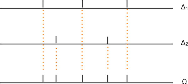
Toy example with two individual partitions {Δ₁} and {Δ₂} and the common partition {Ω}.

Let g_j ∈ {1, 2} indicate the disease subtype for sample j. In our motivating example, g_j = 1 denotes the ER+ subtype and g_j = 2 denotes the TN subtype of breast cancer. We also define some distribution notations: N(μ, σ²) denotes a normal distribution with mean μ and variance σ²; N_p(μ, Σ) is a p-variate multivariate normal distribution with mean μ and variance–covariance matrix Σ; Ga(α, β) is a gamma distribution with mean α/β; IGa(α, β) represents an inverse gamma distribution with mean β/(α −1); and Ber(π) denotes a Bernoulli distribution with success parameter π. $\mathcal{D}\mathcal{P}\left(a,F\right)$ is a Dirichlet process with precision parameter a and centering measure F. We proceed with the introduction of a sampling model, followed by the priors.

2.2 Probability model

With the two aforementioned objectives in mind, we construct the following hierarchical models. Let Y_ij be the log₂ ratio of probe t_i at sample j. We assume that Y_ij arises from the sum of a population mean, a sample-specific mean, plus a measurement error. Specifically, let the population mean be ${\mu }_{k,g_j}$, if probe t_i is in the population segment Ω_k and sample j is from disease subtype g_j; let m_lj be a random effect specific to sample j, assuming that probe t_i is in sample-specific segment Δ_lj; and denote the measurement error by ε_ij. For simplicity, let us assume that t_i = i. In summary, the model has a linear expression of the form

$$Y_{ij}={\displaystyle \sum _{k=1}^K{\mu }_{k,g_j}I\left(I\in {\mathrm{\Omega }}_k\right)+{\displaystyle \sum _{l=1}^{L_j}{m}_{lj}I\left(i\in {\mathrm{\Delta }}_{lj}\right)+{\epsilon }_{ij}}},$$ (2.1)

for i = 1, …, n_j and j = 1, …, J. We assume that the measurement errors ε_ij are independent and identically distributed $\text{N(}0,{\sigma }_{\epsilon }^2\text{)}$.

We set up the following prior distributions to fulfill our objectives. Denote by μ_k = (μ_k1, μ_k2) the vector of population copy number levels for subtypes 1 and 2, respectively, with distribution G. We construct G as a mixture of two distributions G₀ and G₁, which in turn are assigned nonparametric Dirichlet process priors. In notation, we have

$$\begin{array}{l}{\mathit{\mu }}_k|G\stackrel{\text{ind}.}{~}G,\text{for}k=1,\dots ,K\\ G=\left(1-\pi \right)G_0+\pi G_1\\ G_r|a_r\stackrel{\text{ind}.}{~}\mathcal{D}\mathcal{P}\left(a_r,F_r\right),r=0,1,\end{array}$$

where a_r and F_r are the precision and centering measure parameters, respectively. Thus, the μ_k’s turn out to be partially exchangeable. For the centering measures of the nonparametric Dirichlet process priors, we take a degenerate bivariate normal on the identity line $F_0\left({\mathit{\mu }}_k\right)=\mathrm{N}({\mu }_{k1}|0,{\lambda }_0^2)I({\mu }_{k1}={\mu }_{k2})$ and a proper bivariate normal F₁(μ_k) = N₂(μ_k | 0, Λ₁), with ${\lambda }_0^2$ as a nonnegative scalar and Λ₁ a positive defined variance–covariance matrix, where we take the covariance to be zero, that is, ${\mathbf{\Lambda }}_1=\text{diag}({\lambda }_1^2,{\lambda }_2^2)$, to ensure identification in the mixture. Note that these choices for the centering measures are equivalent to the well-known spike and slab priors (e.g., Mitchell and Beauchamp, 1988) but in two dimensions.

The mixture construction G = (1 − π)G₀ + πG₁ and the centering measures for $\mathcal{D}\mathcal{P}$, F₀ and F₁, allow us to determine regions along the chromosome for which the two subgroups manifest different copy numbers. That is, with prior probability (1−π), the random distribution G comes from a DP with a degenerated centering measure F₀, where μ_k1 = μ_k2 almost surely. With prior probability π, the random distribution G comes from a DP with a centering measure that obeys a bivariate normal law, for which μ_k1 ≠ μ_k2 almost surely (see the Appendix for a simple proof). Therefore, introducing a latent indicator z_k = I (μ_k1 ≠ μ_k2) and assuming Pr(z_k = 1) = π, we can rewrite the prior for μ as

$${\mathit{\mu }}_k|z_k,G_0,G_1\stackrel{\text{ind}.}{~}{G}_{z_k},\text{with}{z}_k\stackrel{\text{ind}.}{~}\text{Ber}(\pi )\text{and}{G}_r\stackrel{\text{ind}.}{~}\mathcal{D}\mathcal{P}\left(a_r,F_r\right),$$ (2.2)

for k = 1, …, K and r = 0, 1. Note that (2.1) and (2.2) define a Dirichlet process mixture model (e.g., MacEachern and Müller, 1998).

Due to the discrete nature of the DP prior, some of the μ_k’s will be identical. In summary, the mean copy numbers of segment k for the two disease subtypes, μ_k1’s and μ_k2, will be clustered in two ways: those segments with the same population copy number levels across the chromosome probes, and those segments with the same population copy number levels across the two disease subtypes.

The model specification is completed with the following prior constructions. For the random effects, m_lj, in (2.1), which account for the heterogeneity in the segment means across samples, we assume that

$$m_{lj}\stackrel{\text{ind}.}{~}\mathrm{N}(0,{\tau }_j^2),\text{with}{\tau }_j^2\stackrel{\mathrm{i}.\mathrm{i}.\mathrm{d}.}{~}\text{IGa}\left({\alpha }_{\tau },{\beta }_{\tau }\right).$$ (2.3)

The sample variance is also assigned a prior distribution of the form ${\sigma }_{\epsilon }^2~\text{IGa}\left({\alpha }_{\sigma },{\beta }_{\sigma }\right)$. Finally, for the precision parameter of the Dirichlet processes in (2.2), we further assume $a_r\stackrel{\mathrm{i}.\mathrm{i}.\mathrm{d}.}{~}\text{Ga}\left(a_{\alpha },b_{\alpha }\right)$, for r = 0, 1.

2.3 Posterior computation

The likelihood function is the density of the joint distribution of Y = {Y_ij}, given by

$$\begin{gathered} f\left(\mathbf{y}|\mathit{\mu },\mathbf{m}\right)={(2\pi {\sigma }_{\epsilon }^2)}^{\left(-1/2\right){\displaystyle {\sum }_{j=1}^J{n}_j}} \\ \times \exp \left[-\frac{1}{2{\sigma }_{\epsilon }^2}{\displaystyle \sum _{j=1}^J{\displaystyle \sum _{i=1}^{n_j}{\left\{y_{ij}-{\displaystyle \sum _{k=1}^K{\mu }_{k{g}_j}I\left(i\in {\mathrm{\Omega }}_k\right)-{\displaystyle \sum _{l=1}^{L_j}{m}_{lj}I\left(i\in {\mathrm{\Delta }}_{lj}\right)}}\right\}}^2}}\right]. \end{gathered}$$

We introduce some notation that will be useful in characterizing the posterior:

$$\begin{gathered} s_{kj}={\displaystyle \sum _{i=1}^{n_j}I\left(i\in {\mathrm{\Omega }}_k\right)},s_{lj}={\displaystyle \sum _{i=1}^{n_j}I\left(i\in {\mathrm{\Delta }}_{lj}\right)}, \\ {s}_{klj}={\displaystyle \sum _{i=1}^{n_j}I\left(i\in {\mathrm{\Omega }}_k\right)I\left(i\in {\mathrm{\Delta }}_{lj}\right),} \\ {s}_{kj}^y={\displaystyle \sum _{i=1}^{n_j}{y}_{ij}I\left(i\in {\mathrm{\Omega }}_k\right),\text{and}}{s}_{lj}^y={\displaystyle \sum _{i=1}^{n_j}{y}_{ij}I\left(i\in {\mathrm{\Delta }}_{lj}\right)}. \end{gathered}$$ (2.4)

We now report the conditional posterior distributions needed to perform Markov chain Monte Carlo simulations.

1. Update (μ_k, z_k)

We will jointly update μ_k and z_k. Based on the Polya urn representation of the DP prior (see the Appendix), we can derive the prior conditional distribution for the pair (μ_k, z_k), given all other pairs (μ_j, z_j)’s for j ≠ k, as

$$\begin{gathered} \left({\mathit{\mu }}_k,z_k\right)|{\mathit{\mu }}_{-k},{\mathbf{z}}_{-k} \\ ~\frac{\pi I\left(z_k=1\right)}{a_1+K_1}\left\{a_1{\mathrm{N}}_2\left({\mathit{\mu }}_k|0,{\mathbf{\Lambda }}_1\right)+{\displaystyle \sum _{j\ne k}^K{\delta }_{{\mathit{\mu }}_j}\left({\mathit{\mu }}_k\right)I\left(z_j=1\right)}\right\} \\ +\frac{\left(1-\pi \right)I\left(z_k=0\right)}{a_0+K_0}\left\{a_0\mathrm{N}\left({\mu }_{k1}|0,{\lambda }_0^2\right)I\left({\mu }_{k1}={\mu }_{k2}\right)+{\displaystyle \sum _{j\ne k}^K{\delta }_{{\mathit{\mu }}_j}\left({\mathit{\mu }}_k\right)I\left(z_j=0\right)}\right\}, \end{gathered}$$

where $K_r={\displaystyle {\sum }_{j\ne k}^{K}I\left(z_j=r\right)}$, r = 0, 1 such that K₀ + K₁ = K − 1. Therefore, the posterior conditional for (μ_k, z_k) is given by

$$\begin{gathered} f\left({\mathit{\mu }}_k,z_k|\mathbf{y},\text{rest}\right)=q_{00}\mathrm{N}\left({\mu }_{k1}|B_0,C_0\right)I\left({\mu }_{k1}={\mu }_{k2}\right)I\left(z_k=0\right) \\ +{\displaystyle \sum _{j\ne k}^K{q}_{0j}{\delta }_{{\mu }_j}\left({\mathit{\mu }}_k\right)I\left(z_j=0\right)I\left(z_k=0\right)} \\ +q_{10}{\mathrm{N}}_2\left({\mu }_k|B_1,C_1\right)I\left(z_k=1\right) \\ +{\displaystyle \sum _{j\ne k}^K{q}_{1j}{\delta }_{{\mu }_j}\left({\mathit{\mu }}_k\right)I\left(z_j=1\right)I\left(z_k=1\right)}, \end{gathered}$$ (2.5)

where

$$\begin{gathered} q_{00}=\frac{a_0\left(1-\pi \right)A_0}{\left(a_0+K_0\right)Q},q_{0j}=\frac{\left(1-\pi \right)D_{0j}}{\left(a_0+K_0\right)Q}, \\ {q}_{10}=\frac{a_1\pi A_1}{\left(a_1+K_1\right)Q},q_{1j}=\frac{\pi D_{1j}}{\left(a_1+K_1\right)Q} \end{gathered}$$

with Q the normalizing constant such that $q_{00}+q_{10}+{\displaystyle {\sum }_{j\ne k}^K\left(q_{0j}+q_{1j}\right)=1}$, and

$$\begin{gathered} \begin{array}{l}{A}_0=\varphi \left\{\left(\frac{{\overline{y}}_{k1}}{{\psi }_{k11}}+\frac{{\overline{y}}_{k2}}{{\psi }_{k22}}\right){\left(\frac{1}{{\psi }_{k11}}+\frac{1}{{\psi }_{k22}}\right)}^{-1}|0,{\left(\frac{1}{{\psi }_{k11}}+\frac{1}{{\psi }_{k22}}\right)}^{-1}+{\lambda }_0^2\right\}, \\ {B}_0=\left(\frac{{\overline{y}}_{k1}}{{\mathbf{\Psi }}_{k11}}+\frac{{\overline{y}}_{k2}}{{\psi }_{k22}}\right)C_0, \\ {C}_0={\left(\frac{1}{{\psi }_{k11}}+\frac{1}{{\psi }_{k22}}+\frac{1}{{\lambda }_0^2}\right)}^{-1}, \\ {D}_{0j}=\varphi \left({\mu }_{j1}|{\overline{y}}_{k1},{\psi }_{k11}\right)\varphi \left({\mu }_{j1}|{\overline{y}}_{k2},{\psi }_{k22}\right),\text{for}j\ne k, \\ {A}_1={\varphi }_2\left({\overline{\mathbf{y}}}_k|0,{\mathbf{\Psi }}_k+{\mathbf{\Lambda }}_1\right), \\ {\mathbf{B}}_1=\left(\begin{array}{l}\frac{{\overline{y}}_{k1}}{{\mathbf{\Psi }}_{k11}}{\left(\frac{1}{{\mathbf{\Psi }}_{k11}}+\frac{1}{{\lambda }_1^2}\right)}^{-1}\hfill \\ \frac{{\overline{y}}_{k2}}{{\mathbf{\Psi }}_{k22}}{\left(\frac{1}{{\mathbf{\Psi }}_{k22}}+\frac{1}{{\lambda }_2^2}\right)}^{-1}\hfill \end{array}\right), \\ {\mathbf{C}}_1=\text{diag}\left\{{\left(\frac{1}{{\psi }_{k11}}+\frac{1}{{\lambda }_1^2}\right)}^{-1},{\left(\frac{1}{{\psi }_{k22}}+\frac{1}{{\lambda }_2^2}\right)}^{-1}\right\}, \\ {D}_{1j}={\varphi }_2\left({\mathit{\mu }}_j|{\overline{\mathbf{y}}}_k,{\mathbf{\Psi }}_k\right),\text{for}j\ne k,\end{array} \end{gathered}$$

where ϕ and ϕ₂ are the univariate and bivariate normal density functions, respectively. Finally,

$${\overline{\mathbf{y}}}_k=\left(\begin{array}{l}\frac{{\displaystyle {\sum }_{j=1}^{J}I(g_j=1)(s_{kj}^y-{\displaystyle {\sum }_{l=1}^{L_j}{m}_{lj}{s}_{klj}})}}{{\displaystyle {\sum }_{j=1}^{J}I(g_j=1)s_{kj}}}\hfill \\ \frac{{\displaystyle {\sum }_{j=1}^{J}I(g_j=2)(s_{kj}^y-{\displaystyle {\sum }_{l=1}^{L_j}{m}_{lj}{s}_{klj}})}}{{\displaystyle {\sum }_{j=1}^{J}I(g_j=2)s_{kj}}}\hfill \end{array}\right)$$

and

$${\mathbf{\Psi }}_k=\left(\begin{array}{cc}\frac{{\sigma }_{\epsilon }^2}{{\displaystyle {\sum }_{j=1}^{J}I\left(g_j=1\right)s_{kj}}}& 0\\ 0& \frac{{\sigma }_{\epsilon }^2}{{\displaystyle {\sum }_{j=1}^{J}I\left(g_j=2\right)s_{kj}}}\end{array}\right)$$

for k = 1, …, K, with s_kj and $s_{kj}^y$ as given in (2.4).

2. Update m_lj

For the specific random effects m_lj, the conditional posterior is given by

$$f(m_{lj}|\mathbf{y},\text{rest})=N(m_{lj}|m^{\ast },{\tau }_{\ast }^2),$$ (2.6)

where $m^{\ast }=\frac{s_{lj}^y-{\displaystyle {\sum }_k{\mu }_{k{g}_j}{s}_{klj}}}{{\sigma }_{\epsilon }^2(s_{lj}/{\sigma }_{\epsilon }^2+1/{\tau }_j^2)}\text{and}{\tau }_{\ast }^2={\left(\frac{s_{lj}}{{\sigma }_{\epsilon }^2}+\frac{1}{{\tau }_j^2}\right)}^{-1},$ for l = 1, …, L_j and j = 1, …, J, where s_lj, $s_{lj}^y$ and s_klj are as given in (2.4).

3. Update ${\sigma }_{\epsilon }^2$

For the measurement error variance ${\sigma }_{\epsilon }^2$, the conditional posterior is given by

$$f({\sigma }_{\epsilon }^2|\mathbf{y},\text{rest})=\text{IGa}({\sigma }_{\epsilon }^2|{\alpha }_{\sigma }^{\ast },{\beta }_{\sigma }^{\ast }),$$ (2.7)

where

$${\alpha }_{\sigma }^{\ast }={\alpha }_{\sigma }+\frac{1}{2}{\displaystyle \sum _{j=1}^J{n}_j}$$

and

$${\beta }_{\sigma }^{\ast }={\beta }_{\sigma }+\frac{1}{2}{\displaystyle \sum _{j=1}^J{\displaystyle \sum _{i=1}^{n_j}{\left\{y_{ij}-{\displaystyle \sum _{k=1}^K{\mu }_{k{g}_j}I(i\in {\mathrm{\Omega }}_k)+{\displaystyle \sum _{l=1}^{L_j}{m}_{lj}I(i\in {\mathrm{\Delta }}_{lj})}}\right\}}^2}}.$$

4. Update ${\tau }_j^2$

For the variance of the specific random effects ${\tau }_j^2$, the conditional posterior depends on only $m_{lj}^2$ and is given by

$$f({\tau }_j^2|m_{kj})=\text{IGa}({\tau }_j^2|{\alpha }_{\tau }^{\ast },{\beta }_{\tau }^{\ast }),$$ (2.8)

where

$${\alpha }_{\tau }^{\ast }={\alpha }_{\tau }+\frac{L_j}{2}\text{and}{\beta }_{\tau }^{\ast }={\beta }_{\tau }+\frac{1}{2}{\displaystyle \sum _{l=1}^{L_j}{m}_{lj}^2}.$$

5. Resampling μ_k

As is customary when dealing with almost surely discrete random measures, as in the case for the Dirichlet process, an acceleration step is required to resample the cluster locations (e.g., Bush and MacEachern, 1996). If we denote by ${\mathit{\mu }}_1^{\ast },\dots ,{\mathit{\mu }}_H^{\ast }$ the distinct values of the μ_k’s, and by $z_1^{\ast },\dots ,z_H^{\ast }$ the corresponding latent indicators, then each ${\mathit{\mu }}_h^{\ast }$, conditional on the cluster configuration (c.c.), needs to be resampled from

$$f\left({\mu }_{h1}^{\ast }|\mathbf{y},\mathrm{c}.\mathrm{c}.,z_h^{\ast }=0,\text{rest}\right)=\mathrm{N}\left({\mu }_{h1}^{\ast }|B_0^{\ast },C_0^{\ast }\right),$$ (2.9)

where

$$B_0^{\ast }={\displaystyle \sum _{\{k:{\mathit{\mu }}_k={\mu }_h^{\ast }\}}\left(\frac{{\overline{y}}_{k1}}{{\psi }_{k11}}+\frac{{\overline{y}}_{k2}}{{\psi }_{k22}}\right)C_0^{\ast }}$$

and

$$C_0^{\ast }={\left\{{\displaystyle \sum _{\{k:{\mathit{\mu }}_k={\mu }_h^{\ast }\}}\left(\frac{1}{{\psi }_{k11}}+\frac{1}{{\psi }_{k22}}\right)+\frac{1}{{\lambda }_0^2}}\right\}}^{-1},$$

if $z_h^{\ast }=0$ and setting μ_h2 = μ_h1; or from

$$f\left({\mathit{\mu }}_h^{\ast }|\mathbf{y},\mathrm{c}.\mathrm{c}.,z_h^{\ast }=1,\text{rest}\right)={\mathrm{N}}_2\left({\mathit{\mu }}_h^{\ast }|{\mathbf{B}}_1^{\ast },{\mathbf{C}}_1^{\ast }\right),$$ (2.10)

where

$${\mathbf{B}}_1^{\ast }=\left(\begin{array}{c}{C}_{111}^{\ast }{\displaystyle \sum _{\{k:{\mathit{\mu }}_k={\mu }_h^{\ast }\}}\frac{{\overline{y}}_{k1}}{{\psi }_{k11}}}\\ C_{122}^{\ast }{\displaystyle \sum _{\{k:{\mathit{\mu }}_k={\mu }_h^{\ast }\}}\frac{{\overline{y}}_{k2}}{{\psi }_{k22}}}\end{array}\right)$$

and

$${\mathbf{C}}_1^{\ast }=\text{diag}\left\{{\left({\displaystyle \sum _{\{k:{\mathit{\mu }}_k={\mu }_h^{\ast }\}}\frac{1}{{\psi }_{k11}}+\frac{1}{{\lambda }_1^2}}\right)}^{-1},{\left({\displaystyle \sum _{\{k:{\mathit{\mu }}_k={\mu }_h^{\ast }\}}\frac{1}{{\psi }_{k22}}+\frac{1}{{\lambda }_2^2}}\right)}^{-1}\right\},$$

if $z_h^{\ast }=1$.

6. Update a_r

Finally, for the precision parameters a_r, r = 0, 1 in the Dirichlet processes, we know from Antoniak (1974) that the conditional posterior distribution of a_r depends on only the number of distinct μ_k’s and the sample size, that is,

$$f\left(a_r|H_r,K_r\right)\propto \frac{\Gamma \left(a_r\right)}{\Gamma \left(a_r+K_r\right)}{a}_r^{H_r+{\alpha }_a-1}{e}^{-{\beta }_a{a}_r},$$ (2.11)

where $K_r={\displaystyle {\sum }_{k=1}^{K}I\left(z_k=r\right)}$ and H_r is the number of distinct values μ_k’s such that z_k = r, for r = 0, 1.

The precision parameter a_r plays a very important role. It largely affects the number of clusters in the μ_k’s. A small value of a_r implies fewer clusters, whereas a large value results in many clusters. Since for the arrayCGH data we anticipate having a relatively small number of segments per chromosome, we will consider relatively informative priors in such a way that they assign most of the mass to small values of a_r.

Sampling from each of the previous conditional posterior distributions is straightforward, since almost all of them have a standard form. The exception is the updating step 6, for which we would require a Metropolis–Hastings step (Tierney, 1994). The main challenge lies in the speed of computation for large data sets, which we have. Programming language such as R will not scale. Instead, we used Fortran, a low-level but much faster language for coding. The computing speed is much improved.

2.4 Calling differential copy number alterations

There are several quantities of interest that we want to focus on in order to achieve our inferential objectives. We break down these quantities into two categories, those for population-level inference, and those for sample-specific inference. The key parameters of interest are μ_k = (μ_k1, μ_k2), z_k, and m_lj.

To obtain summaries at the population level, for each population segment k = 1, …, K, we compute marginal posterior probabilities for each disease subtype, say p₁ = P(|μ_k1| ≥ d₁ | data) and p₂ = P(|μ_k2 | ≥d₂ | data), for given values of d₁ and d₂. Higher values of these probabilities will imply a marginal CNA for each subtype.

Moreover, to determine differential CNAs across disease subtypes, we compute the joint posterior probabilities,

$$p_z=\mathcal{P}\left(\left\{\left|{\mu }_{k1}\right|\ge d_1\text{or}\left|{\mu }_{k2}\right|\ge d_2\right\},\left\{z_k=1\right\}|\text{data}\right),$$

for k = 1, …, K. Higher values of these probabilities indicate that segment k has CNAs in any of the disease subtypes and there are differential copy numbers across the two subtypes. The different combinations given in the previous description of the probability may also produce alternative inferences. The threshold to determine high probability values for p₁, p₂ and p_r is set according to a prespecified FDR.

For the sample-specific inference, for each sample j and segment l, the segment-specific mean copy number is $({\mu }_{k,g_j}+m_{l,j})$, in which the population segment k overlaps with the sample-specific segment. Note that there can be several population segments that are embedded in the same sample-specific segment. When this is the case, we simply report inference according to the segments defined by the population segments.

3 Data analysis

In this section, we consider two analyses, one with simulated data under different scenarios to test our model, and the other with real data obtained from a breast cancer study conducted at MD Anderson Cancer Center.

3.1 Simulated data

We implemented a simulation study in order to evaluate the operating characteristics of our approach. We simulated samples with n = 1000 probes, with ordered locations ranging from 1 to n. For group g = 1, we considered four regions of shared aberrations around locations {200, 400, 600, 800}, alternating gain and loss. Group g = 2 contains only two regions of aberration at locations {600, 800} identified as a copy number gain and loss, respectively. We randomly generated aberration widths from a Ga(2.5, 0.05) distribution that has a mean of 50 and 99% interval (5, 168), which shows a large variability and accommodates both large and short segments. We took the level of the profiles for each probe to be zero for the neutral zones and to be a positive/negative random value Un(0.1, 0.25) for the gain/loss zones, respectively.

We then added white noise to these mean profiles. We generated random errors from N(0, σ²), with σ² ∈ {0.1, 0.3} to show low and high levels of noise in the log₂ ratios. We generated 100 profiles, 50 from each group. To test our model under different conditions, only a percentage ω100% of the profiles presented the shared aberrations; the remainder (1−ω)100% were all neutral, showing only white noise around zero. We took three prevalence levels, ω ∈ {1, 0.6, 0.3}. Therefore, we have a total of 6 different scenarios. Scenarios 1 to 3 have low noise with 100%, 60% and 30% prevalence levels, respectively, and scenarios 4 to 6 have high noise with 100%, 60% and 30% prevalence levels, respectively.

Figure 2 shows four profiles for the low (left column) and high (right column) noise levels. We can see that for the high noise profiles, it is very difficult to distinguish (visually) the aberration zones. In the same figure, we present group 1, with four aberration zones (top row) and group 2, with only two aberration zones (bottom row).

Figure 2.

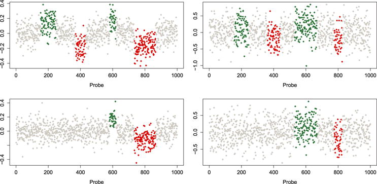
Simulated aCGH data. No copy number alterations (white dots), amplifications (green/medium grey dots) and deletions (red/dark grey dots). Group 1 (top row) and group 2 (bottom row). Low noise level (left column) and high noise level (right column).

To obtain the sample-specific partitions {Δ_lj}, we ran the CBS algorithm with the default tuning parameter α = 0.01. We fitted our model with the following prior specifications: ${\lambda }_0^2={\lambda }_1^2={\lambda }_2^2=100$ to induce flat centering measures, and (α_a, β_a) = (1, 1) as a relatively informative prior to induce a small a_r, and thus a low number of point masses in the Dirichlet processes. For the inverse gamma prior on the sampling variance ${\sigma }_{\epsilon }^2$, we took (α_σ, β_σ) = (2, 1) to be a little informative. The crucial parameter in the model is the variance of the segment-specific random effects, ${\tau }_j^2$. Large values of ${\tau }_j^2$ would make the sample-specific effects capture most of the variability of the data, leaving little information for the population mean. On the other hand, if ${\tau }_j^2$ is small, the variability of the data is shared between the population effects and the sample-specific effects. In fact, if we choose (α_τ, β_τ) = (2, 1), the logarithm of the pseudo marginal likelihood (LPML) statistic (Geisser and Eddy, 1979) for scenario 1 is 88, 686; whereas if (α_τ, β_τ) = (3, 0.01), the LPML is 80, 211. Although the fitting of the individual samples is better with the former choice, we prefer the latter because it produces better estimates for both the population and individual samples. In all cases, we ran the Gibbs sampler for 10,000 iterations with a burn-in of 1000, keeping every other draw after burn-in for computing the estimates. The Markov chain converged quickly and mixed well.

For calling differential CNAs, we took FDR = 5%, with thresholds d₁ = d₂ = d. Since we have different levels of prevalence of aberrations in the samples, in the different scenarios, it is more difficult to call a CNA. To be fair, we took d = 0.10, 0.05, 0.03 as threshold values for the 100%, 60% and 30% prevalence levels, respectively.

Figure 3 presents the CNA calls for the different scenarios. In each panel, we show three rectangles, with the x-axis indicating the probe location. The first two rectangles correspond to the marginal CNAs of groups 1 and 2 called from p₁ and p₂. The third rectangle indicates the regions along the chromosome where there are CNA differences across the two chromosomes, called from p_z. As we can see from this figure, with a low level of noise in the data, our model is able to detect the regions of aberration in each group, as well as the regions of CNA differences across the two groups, for the three prevalence scenarios.

Figure 3.

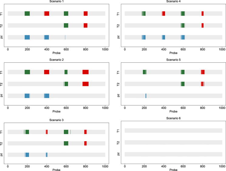
Simulated aCGH data. Calls of marginal CNAs and differences between the two groups (T1 and T2). Copy number gain (green/medium grey), loss (red/dark grey) and differential CNAs across groups (blue/light grey). Low noise level (left column) and high noise level (right column). Prevalence levels: 100% (top row), 60% (middle row) and 30% (bottom row).

Now, looking at the right column in Figure 3, which corresponds to the scenario of a high noise level, our model is able to detect most marginal regions of aberrations for the cases with 100% and 60% prevalence; however, it is not able to detect any of the aberrations in the cases with low prevalence. This is reasonable because, given 30% aberration prevalence in the samples combined with a high noise level, the findings are essentially white noise. For the 100% aberration prevalence in the samples (top right panel in Figure 2), we notice that even though our model correctly detects the marginal regions of aberrations in each group, it also detects a difference in the levels of the second region of amplifications, denoted with a blue/light grey segment aligned with the two green/medium grey segments in groups 1 and 2. This false discovery is also due to the high level of noise present in the data.

To study the dependence of our model to the sample specific partitions {Δ_lj}, we repeated the analysis with other two values of the tuning parameter α in the CBS algorithm, say 0.001 and 0.05. With a smaller value of α, CBS detects less changing points, whereas with a larger value, more changing points are detected. Results (not included here) showed that the impact of the partitions in the inference is almost null, perhaps it is preferred a partition with more segments (larger α in the CBS) than another with few segments, specially when the level of prevalence is low.

3.2 Breast cancer data

At the University of Texas MD Anderson Cancer Center, we conducted arrayCGH experiments using samples from 122 patients with breast cancer. For each sample, we used an Agilent HG 4×44K array with 42,416 unique probes. As a result, the raw data contained a matrix of 42,416 × 122 log₂ ratios. The tumor samples we analyzed represented 60 patients with ER+ breast cancer, 11 patients with PR+ breast cancer, and 51 patients with TN breast cancer. Given the reduced number of patients with the subtype PR+, we concentrated on comparing the other two subtypes, ER+ and TN. It is common practice to analyze each chromosome separately since it is rare to see cross-chromosomal CNAs. Therefore, we split the data based on the chromosomes and analyzed each of them separately.

To prepare for Bayesian inference, we preprocessed the arrayCGH data, which included a global normalization process to center the sample mean for each of the 111 samples. Analogous to the simulated data, we obtained sample-specific partitions {Δ_lj} by running the CBS algorithm with a tuning parameter of α = 0.01. We used the same prior specifications that we used in the simulated data analysis. We ran the Gibbs samplers for 10,000 iterations, with a burn-in of 1000, keeping every other draw. Again, for calling a differential CNA, we took FDR = 5%, with thresholds d₁= d₂ = 0.2 for all chromosomes. We found CNA differences between the two cancer subtypes in 16 of the 23 chromosomes; predominantly in chromosomes 3–7, 9–12, 14–19 and 23.

In Figures 4 and 5, we present marginal CNAs for the two cancer subtypes (ER+ and TN) and copy number differences across the two subtypes.

Figure 4.

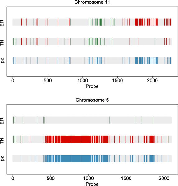
Calls of marginal CNAs and differences between the two cancer subtypes. Copy number gain (green/medium grey), loss (red/dark grey) and differential CNAs across groups (blue/light grey). Chromosomes 11 (top) and 5 (bottom).

Figure 5.

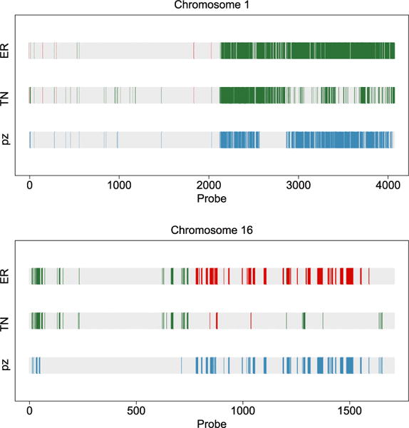
Calls of marginal CNAs and differences between the two cancer subtypes. Copy number gain (green/medium grey), loss (red/dark grey) and differential CNAs across groups (blue/light grey). Chromosomes 1 (top) and 16 (bottom).

Curtis et al. (2012) provided what is perhaps the most comprehensive report on genomic architecture for breast cancer, based on genomics findings from a study of 2000 breast tumors. We compared our statistical inference with the findings in that article, and report the results below.

An ER+ subgroup of breast cancer found in Curtis et al. (2012) is uniquely marked by 11q deletion. This subgroup of patients exhibited a steep mortality rate and elevated hazard ratios in the findings of Curtis et al. The top panel of our Figure 4 clearly shows the deletion to chromosome 11 in the second half, marked by the red bars. These deletions are not present in the TN subgroup, echoing the findings of Curtis et al. (2012). Furthermore, the green/medium grey bars in the middle of chromosome 11 indicate copy number gains in this region, which was also reported by Curtis et al. However, these copy number gains are present in both the ER+ and TN groups, making them less interesting for distinguishing the two subgroups. The bottom panel of our Figure 4 shows a large chunk of copy number loss on chromosome 5, which is unique to the TN subgroup. This is one of the major findings of Curtis et al., as well. This is a region containing numerous important signaling molecules and transcription factors, the aberration of which not only affects the genes residing in the region, but those regulated by them. Therefore, this is marked as a trans-influenced region by Curtis et al. (2012).

The two plots in our Figure 5 show a classical 1q gain and 16q loss pattern that is shared by luminal A breast cancer, a subgroup of the ER+ subtype. The combination of copy number gain of 1q and loss of 16q is believed to be a centromere-close translocation (Russnes et al., 2010), which is mainly seen in the luminal A subgroup. In contrast, there is little copy number variation on 16q for the TN subgroup.

We identified several other new findings regarding the copy number variations between the ER+ and TN subgroups. For example, a large region of 15p loss (Figure 6) is identified in the TN subgroup, but not the ER+ subgroup. This has not been reported in the literature. However, in Figure 2 on page 12 in Curtis et al. (2012), a copy number loss at 15q is present. Figure 7 summarizes the differential CNA probabilities between groups for the whole genome. We believe that our findings confirm several major results reported in the literature, while also providing new hypotheses for future validations.

Figure 6.

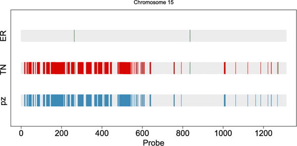
Calls of marginal CNAs and differences between the two cancer subtypes in chromosome 15. Copy number gain (green/medium grey), loss (red/dark grey) and differential CNAs across groups (blue/light grey).

Figure 7.

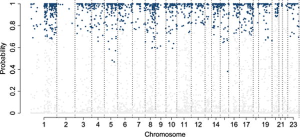
Differential CNA probabilities between groups for all chromosomes. Blue/grey lines represent significant probabilities controlled by a 5% FDR within each chromosome.

4 Discussion

Determining regions of shared CNAs in different samples is a challenging task and is of great importance for the advance of medical science. In this article, we addressed the problem of determining shared CNAs based on a two step model with the second step based on a semiparametric model. The model is equipped with the ability to identify differences along the genome where two disease subtypes show differential CNAs. This was achieved by considering a mixture distribution for the vector of the population levels, the elements of which were in turn assigned Dirichlet process priors.

Through simulation studies, we have shown that the proposed model adequately determines the shared aberration regions and detects the differences across the two subgroups. The model was tested under different levels of aberration prevalence and with different degrees of noise. In most of the scenarios we considered, our model worked well. The exception occurred in scenarios with a combination of high noise level and low aberration prevalence, which is an expected finding. We also found out that the sample specific partitions have almost no influence in the final inferences.

Future work includes the extension of our model to compare more than two groups, for which the number of possible combinations then increases dramatically. For example, in the case of three groups, we would have to consider a total of five cases: the three groups as equal, any two as equal, and all as different. This will entail a nontrivial generalization of our mixture prior set-up, a task we will undertake in the future.

Appendix

Stick breaking and Polya urn representation of a $\mathcal{D}\mathcal{P}$

In general, a Dirichlet process G, such that $G~\mathcal{D}\mathcal{P}\left(a,F\right)$, is a random discrete measure with precision parameter a and centering measure F. According to Sethuraman (1994), G can be written as a stick breaking representation of the form

$$G(\cdot )={\displaystyle \sum _{h=1}^{\mathrm{\infty }}{w}_h{\delta }_{{\eta }_h}(\cdot )},$$

where δ_x(·) defines a point mass at x, ${\eta }_h\stackrel{\mathrm{i}.\mathrm{i}.\mathrm{d}.}{~}F$ and w_h = v_h∏_j<h(1 − v_j), with $v_h\stackrel{\mathrm{i}.\mathrm{i}.\mathrm{d}.}{~}\text{Be}\left(1,a\right)$. Additionally, if ${\mathit{\mu }}_1,\dots ,{\mathit{\mu }}_K|G\stackrel{\mathrm{i}.\mathrm{i}.\mathrm{d}.}{~}G$, then after integrating out the process G, Blackwell and MacQueen (1973) showed that the sequence of μ_k’s has a Polya urn representation of the form

$$\begin{gathered} {\mathit{\mu }}_1~F; \\ {\mathit{\mu }}_k|{\mathit{\mu }}_1,\dots ,{\mathit{\mu }}_{k-1}~\frac{a}{a+k-1}F+\frac{1}{a+k-1}{\displaystyle \sum _{j=1}^{k-1}{\delta }_{{\mathit{\mu }}_j}}, \end{gathered}$$

for k = 2, …, K. Denoting by μ = (μ₁, …, μ_K) and by μ_−k = μ \ {μ_k}, it can be easily shown that

$$\begin{gathered} {\mathit{\mu }}_k|{\mathit{\mu }}_{-k}~\frac{a}{a+K-1}F+\frac{1}{a+K-1}{\displaystyle \sum _{j=1,j\ne k}^K{\delta }_{{\mathit{\mu }}_j}}, \\ ~\frac{a}{a+K-1}F+\frac{1}{a+K-1}{\displaystyle \sum _{j=1}^r{K}_j^{\ast }{\delta }_{{\mathit{\mu }}_j^{\ast }}}, \end{gathered}$$

where ${\mathit{\mu }}_j^{\ast }$’s are the distinct values of μ_k’s and $K_j^{\ast }$’s are the numbers of repetitions. By the above construction, it is easy to show that when $F=F_0=\mathrm{N}(0,{\lambda }_0^2)I({\mu }_{k1}={\mu }_{k2})$, almost surely μ_k1 = μ_k2. Alternatively, if F = F₁ = N₂(0, Λ₁), almost surely μ_k1 ≠ μ_k2.

References

- Antoniak CE. Mixtures of Dirichlet processes with applications to Bayesian nonparametric problems. The Annals of Statistics. 1974;2:1152–1174. [Google Scholar]
- Baladandayuthapani V, Ji Y, Talluri R, Nieto-Barajas LE, Morris JS. Bayesian random segmentation models to identify shared copy number aberrations for array CGH data. Journal of the American Statistical Association. 2010;105:1358–1375. doi: 10.1198/jasa.2010.ap09250. [DOI] [PMC free article] [PubMed] [Google Scholar]
- Blackwell D, MacQueen JB. Ferguson distributions via Pólya urn schemes. The Annals of Statistics. 1973;1:353–355. [Google Scholar]
- Bush CA, MacEachern SN. A semiparametric Bayesian model for randomized block designs. Biometrika. 1996;83:275–285. [Google Scholar]
- Curtis C, Shah SP, Chin SF, Turashvili G, Rueda OM, Dunning MJ, et al. The genomic and transcriptomic architecture of 2,000 breast tumours reveals novel subgroups. Nature. 2012;486:346–352. doi: 10.1038/nature10983. [DOI] [PMC free article] [PubMed] [Google Scholar]
- Eilers PHC, de Menezes RX. Quantile smoothing of array CGH data. Bioinformatics. 2005;21:1146–1153. doi: 10.1093/bioinformatics/bti148. [DOI] [PubMed] [Google Scholar]
- Ferguson TS. A Bayesian analysis of some nonparametric problems. The Annals of Statistics. 1973;1:209–230. [Google Scholar]
- Fridlyand J, Snijders AM, Pinkel D, Albertson DG, Jain AN. Hidden Markov models approach to the analysis of the array CGH data. Journal of Multivariate Analysis. 2004;90:132–153. [Google Scholar]
- Geisser S, Eddy WF. A predictive approach to model selection. Journal of the American Statistical Association. 1979;74:153–160. [Google Scholar]
- Guha S, Li Y, Neuberg D. Bayesian hidden Markov modeling of array CGH data. Journal of the American Statistical Association. 2008;103:485–497. doi: 10.1198/016214507000000923. [DOI] [PMC free article] [PubMed] [Google Scholar]
- Hodgson G, Hager J, Volik S, Hariono S, Wernick M, Moore D, et al. Genome scanning with array CGH delineates regional alterations in mouse islet carcinomas. Nature Genetics. 2001;929:459–464. doi: 10.1038/ng771. [DOI] [PubMed] [Google Scholar]
- Huang T, Wu B, Lizardi P, Zhao H. Detection of DNA copy number alterations using penalized least squares regression. Bioinformatics. 2005;21:3811–3817. doi: 10.1093/bioinformatics/bti646. [DOI] [PubMed] [Google Scholar]
- MacEachern SN, Müller P. Estimating mixture of Dirichlet process models. Journal of Computational and Graphical Statistics. 1998;7:223–239. [Google Scholar]
- Mitchell TJ, Beauchamp JJ. Bayesian variable selection in linear regression. Journal of the American Statistical Association. 1988;83:1023–1032. [Google Scholar]
- Newton MA, Noueiry A, Sarkar D, Ahlquist P. Detecting differential gene expression with a semiparametric hierarchical mixture method. Biostatistics. 2004;5:155–176. doi: 10.1093/biostatistics/5.2.155. [DOI] [PubMed] [Google Scholar]
- Olshen AB, Venkatraman ES, Lucito R, Wigler M. Circular binary segmentation for the analysis of array-based DNA copy number data. Biostatistics. 2004;4:557–572. doi: 10.1093/biostatistics/kxh008. [DOI] [PubMed] [Google Scholar]
- Pinkel D, Albertson DG. Array comparative genomic hybridization and its applications in cancer. Nature Genetics. 2005;37:11–17. doi: 10.1038/ng1569. [DOI] [PubMed] [Google Scholar]
- Pinkel D, Segraves R, Sudar D, Clark S, Poole I, Kowbel D, et al. High resolution analysis of DNA copy number variation using comparative genomic hybridization to microarrays. Nature Genetics. 1998;20:207–211. doi: 10.1038/2524. [DOI] [PubMed] [Google Scholar]
- Pollack JR, Sorlie T, Perou C, Rees C, Jeffrey S, Lonning P, et al. Microarray analysis reveals a major direct role of DNA copy number alteration in the transcriptional program of human breast tumors. Proceedings of the National Academy of Sciences of the United States of America. 2002;99:12963–12968. doi: 10.1073/pnas.162471999. [DOI] [PMC free article] [PubMed] [Google Scholar]
- Russnes HG, Vollan HK, Lingjaerde OC, Krasnitz A, Lundin P, Naume B, et al. Genomic architecture characterizes tumor progression paths and fate in breast cancer patients. Science Translational Medicine. 2010;2:1–13. doi: 10.1126/scitranslmed.3000611. [DOI] [PMC free article] [PubMed] [Google Scholar]
- Sethuraman J. A constructive definition of Dirichlet priors. Statistica Sinica. 1994;4:639–650. [Google Scholar]
- Shah SP, Lam WL, Ng RT, Murphy KP. Modeling recurrent DNA copy number alterations in array CGH data. Bioinformatics. 2007;23:450–458. doi: 10.1093/bioinformatics/btm221. [DOI] [PubMed] [Google Scholar]
- Snijders AM, Nowak N, Segraves R, Blackwood S, Brown N, Conroy J, et al. Assembly of microarrays for genome-wide measurement of DNA copy number. Nature Genetics. 2001;29:263–264. doi: 10.1038/ng754. [DOI] [PubMed] [Google Scholar]
- Teo SM, Pawitan Y, Kumar V, Thalamuthu A, Seielstad M, Chia KS, Salim A. Multi-platform segmentation for joint detection of copy number variants. Bioinformatics. 2011;27:1555–1561. doi: 10.1093/bioinformatics/btr162. [DOI] [PubMed] [Google Scholar]
- Tibshirani R, Wang P. Spatial smoothing and hot spot detection for CGH data using the fused lasso. Biostatistics. 2008;9:18–29. doi: 10.1093/biostatistics/kxm013. [DOI] [PubMed] [Google Scholar]
- Tierney L. Markov chains for exploring posterior distributions. The Annals of Statistics. 1994;22:1701–1722. [Google Scholar]
- Yau C, Papaspiliopoulos O, Roberts G, Holmes C. Bayesian non-parametric hidden Markov models with applications in genomics. Journal of the Royal Statistical Society, Series B. 2011;73:37–57. doi: 10.1111/j.1467-9868.2010.00756.x. [DOI] [PMC free article] [PubMed] [Google Scholar]
- Zhang Z, Lange K, Sbatti C. Reconstructing DNA copy number by joint segmentation of multiple sequences. BMC Bioinformatics. 2012;13:205. doi: 10.1186/1471-2105-13-205. [DOI] [PMC free article] [PubMed] [Google Scholar]