Abstract
Harmful algal blooms of cyanobacteria (CyanoHAB) have emerged as a serious environmental concern in large and small water bodies including many inland lakes. The growth dynamics of CyanoHAB can be chaotic at very short timescales but predictable at coarser timescales. In Lake Erie, cyanobacteria blooms occur in the spring-summer months, which, at annual timescale, are controlled by the total spring phosphorus (TP) load into the lake. This study aimed to forecast CyanoHAB cell count at sub-monthly (e.g., 10-day) timescales. Satellite-derived cyanobacterial index (CI) was used as a surrogate measure of CyanoHAB cell count. CI was related to the in-situ measured chlorophyll-a and phycocyanin concentrations and Microcystis biovolume in the lake. Using available data on environmental and lake hydrodynamics as predictor variables, four statistical models including LASSO (Least Absolute Shrinkage and Selection Operator), artificial neural network (ANN), random forest (RF), and an ensemble average of the three models (EA) were developed to forecast CI at 10-, 20- and 30-day lead times. The best predictions were obtained by using the RF and EA algorithms. It was found that CyanoHAB growth dynamics, even at sub-monthly timescales, are determined by coarser timescale variables. Meteorological, hydrological, and water quality variations at sub-monthly timescales exert lesser control over CyanoHAB growth dynamics. Nutrients discharged into the lake from rivers other than the Maumee River were also important in explaining the variations in CI. Surprisingly, to forecast CyanoHAB cell count, average solar radiation at 30 to 60 days lags were found to be more important than the average solar radiation at 0 to 30 days lag. Other important variables were TP discharged into the lake during the previous 10 years, TP and TKN discharged into the lake during the previous 120 days, the average water level at 10-day lag and 60-day lag.
Keywords: Harmful algal blooms, Machine learning, Forecasting, Lake Erie, Freshwater lakes
1. Introduction
Occurrences of harmful algal blooms (HABs), especially of cyanobacteria (CyanoHAB), have increased across the globe because of eutrophication of water bodies, increasing CO2, and rising global temperatures (Huisman et al., 2018; Ho et al., 2019). CyanoHABs pose a threat to both ecological stability (Paerl and Otten, 2013) and drinking water sources (Kotut et al., 2006; Handler et al., 2023). Therefore, effective mitigation of CyanoHABs will be crucial for environmental management in the future. Several mitigation measures such as nutrient management (Fastner et al., 2016), artificial mixing of water (Visser et al., 2016), or shortening the residence time of water (Mitrovic et al., 2011) have been attempted on different lakes with varying success. For an effective mitigation strategy – what measures to implement and when to implement them - it is important to forecast whether the CyanoHAB would occur or not, and if so, with what intensity.
The predictability of CyanoHAB cell count depends upon the timescale under consideration. At very short timescales, the algae growth dynamics can be chaotic (Scheffer et al., 2003). At annual timescales, CyanoHAB cell count may be predictable using nutrient load, ambient temperatures, residence time of water in the lake, etc. as predictors (Stumpf et al., 2012; Michalak et al., 2013). At intermediate timescales (daily to monthly), however, the predictability of CyanoHAB cell count has not been established yet. At sub-monthly timescales, the growth of CyanoHAB is determined by water temperature, wind speed, turbulent mixing, nutrient availability, depth of water column, available solar radiation, the residence time of water, competition with other algal species, presence of zooplankton, etc. (Huisman et al., 2018; Wilhelm et al., 2020). Typically, accurate data on all these variables are unavailable, and at any rate, the available data provide only approximate estimates of these variables. For example, data on nutrients discharged by the various rivers flowing into Lake Erie are available (Heidelberg Tributary Loading Program, NCWQR, 2022), but the information about spatial distribution of the nutrients within the lake, which is important to model growth dynamics (Chaffin et al., 2013), may be unavailable. Similarly, the water temperature may not always be directly available and one may have to use ambient air temperature as a surrogate for water temperature. Statistical methods can be very useful to forecast CyanoHAB intensity using available data.
A data-driven model that can forecast CyanoHAB intensity at sub-monthly timescales would be a useful complement to satellite-monitored CyanoHAB data to help formulate effective mitigation strategies (Millie et al., 2014; Franks, 2018; Rousso et al., 2020; Deng et al., 2021). Such a model may also be used to examine ‘what if’ scenarios for the control and management of CyanoHAB outbreaks. Satellites capture the spatial distribution of CyanoHAB cells over an entire lake as opposed to in-situ data which may not provide a holistic picture of the lake. Typically, Sentinel-3 data provides one image over the time period of 1–2 days at a pixel resolution of approximately 300m × 300m. Satellite data, along with other environmental data, may be used to forecast the CyanoHAB intensity in the near future. A lake hydrodynamic model may also be used to simulate the transport of algal particles with initial conditions specified by a cloud-free image (Soontiens et al., 2019). These simulations, however, neglect the growth and mortality of CyanoHAB at short timescales (daily and sub-monthly; Ranjbar et al., 2021). Indeed, for some CyanoHAB species, the growth rate is typically <0.1 day−1 (Fahnenstiel et al., 2008), but the growth rates can reach up to 0.67 day−1 (Reitz, 2020) and mortality may be an important factor in some cases (e.g., Soontiens et al., 2019). Models for the sub-daily growth of CyanoHAB cells (e.g., Verhamme et al., 2016) that simulate complex interactions between different elements of CyanoHAB growth dynamics tend to be computationally very demanding (Ranjbar et al., 2021) and are not well suited for short-term forecasts because of time constraints.
In addition, uncertainties associated with several variables cannot be assessed easily. Hydrodynamic models are based upon numerical solutions of Navier-Stokes equations (often with simplifying assumptions) that require the specification of boundary and initial conditions (Welander, 1957; Cheng et al., 1976; Bengtsson, 1978; Leon et al., 2011; Beletsky et al., 2013). The solution of Navier-Stokes equations yields the velocity field. To model CyanoHAB growth dynamics, one also requires the evolution of the temperature field and other variables associated with the transport of CyanoHAB cells within the lake such as the coefficient of turbulent dispersion. The values of these variables themselves vary in space. Typically, a fixed value of these variables is used which introduces additional uncertainty in the modeling effort. A data-driven model that can forecast CyanoHAB cell count at sub-monthly timescales would be a good addition to our toolbox.
The focus of this research is Lake Erie, and the main goal is to investigate if near-future CyanoHAB cell count can be forecasted using currently available hydro-meteorological and environmental data, and satellite-derived current CyanoHAB cell count. Lake Erie is one of the five Great Lakes in North America and is the shallowest of the five lakes (Reutter, 2019). Because of the large loads of nutrients discharged into the lake from the agriculturally intensive Maumee River watershed (Muenich et al., 2016), the lake frequently hosts blooms of cyanobacteria, especially in its western part (Chaffin et al., 2011; Michalak et al., 2013; Wynne and Stumpf, 2015). The dominant species of cyanobacteria in the lake is Microcystis aeruginosa (M. aeruginosa) which releases a toxic compound called microcystin (Rinta-Kanto et al., 2009; Stumpf et al., 2016), potentially fatal to humans and aquatic life.
The species M. aeruginosa can control its buoyancy (Kromkamp et al., 1988; You et al., 2018). When wind speed is low and water is calm, this species stays on the water surface which helps it grow by directly absorbing solar radiation and outcompeting other phytoplankton species (Wallace et al., 2000; Den Uyl et al., 2021). During stronger winds, the vertical turbulent mixing force in the lake overcomes the buoyancy of M. aeruginosa, and as a result, they are vertically mixed throughout the lake depth in the western part of Lake Erie. In this situation, effectively less solar radiation is absorbed by the CyanoHAB population and hence cell growth rate decreases. Moreover, experiments show that CyanoHAB growth is optimum when the ambient temperature is between 15–35°C and the growth rate peaks at a temperature within this range (Paerl and Huisman, 2009).
In this study, three types of data were collected: (1) CyanoHAB cell count in Lake Erie during the months of May to October, (2) Nutrients discharged into the lake from inflowing rivers, and (3) Meteorology and hydrodynamics of Lake Erie. A proxy for CyanoHAB cell count, referred to as cyanobacterial index (CI, Wynne et al., 2010), was computed using Medium Resolution Imaging Spectroradiometer (MERIS) and Sentinel-3 OLCI (Ocean and land Cover Instrument) satellite observations. MERIS and Sentinel-3 satellites capture instantaneous images of Lake Erie every 2–3 days and 1–2 days, respectively, but several images contain missing values due to cloud cover and may not accurately reflect CyanoHAB cell count. Therefore, 10-day composite images (Stumpf et al., 2012; Mishra et al., 2019) were created to obtain an estimate of CyanoHAB cell count such that the value obtained represents CyanoHAB cell counts during a period of 10 days. Thus, the scale of measurement of CyanoHAB cell count is 10 days in this study. Nutrient data include various forms of phosphorus and nitrogen loads discharged into the lake from four major rivers contributing nutrients to the Lake (Sayers et al., 2016; Muenich et al., 2016): Maumee, Raisin, Sandusky, and Cuyahoga. Detroit River is the largest river draining into Lake Erie but discharge data from this river are available only since Oct 2008 which will substantially reduce the amount of data available to develop data-driven models. Also, the discharges in the Detroit River stay approximately constant during the month of May to Oct except for some random variations; therefore, these are unlikely to help develop a more accurate ML model for short timescale forecasts. Additionally, nutrient data for the Detroit River are exceedingly sparse (less than 200 point observations in 20 years). Importantly for this study, the largest source of nutrients in the lake is the Maumee River (Baker et al., 2014; Stow et al., 2015). Consequently, the Detroit River data were excluded from the analysis.
Meteorological and hydrological data included wind speed, lake water level, solar radiation, residence time of water, and air temperature over Lake Erie, etc. The goal is to investigate whether one can forecast CyanoHAB cell counts in Lake Erie with 10-, 20- and 30-day lead time using these data and, if so, to identify the variables that help explain the variation in CyanoHAB cell count. CI has been empirically related to CyanoHAB cell count in Lake Erie (Wynne et al., 2010). Although there was a significant scatter in the relationship developed by Wynne et al. (2010), it appears to be a good relation given the errors associated with the estimation of cell count and computations of CI. In this study, the relationships between CI and in-situ measures of CyanoHAB cell count were explored further. Specifically, the study objectives were:
To develop relationships between CI and in-situ measured concentrations of CyanoHAB pigments,
To develop and evaluate three distinct data-driven models and their ensemble average for forecasting CI (a surrogate for CyanoHAB cell count) in Lake Erie at lead times 10, 20, and 30 days,
To identify the important variables for the forecasting of CI.
Three machine learning (ML) models were developed to forecast CI: LASSO (Least Absolute Shrinkage and Selection Operator), random forest (RF), and artificial neural networks (ANNs). LASSO is a linear model with the capability to eliminate redundant variables. RF and ANN can identify the non-linear relationships between response and predictor variables but require more data. RF and ANN have different conceptual underpinnings which may result in different capabilities of these models in providing a forecast. A weighted average of these models, referred to as the ensemble-average (EA) model, was also considered for forecasting CI values.
In this study, the predictive uncertainty of the models was also estimated based on residual analysis. An appropriate statistical distribution was fitted to the residuals obtained by the different models and prediction intervals were obtained based on the fitted residuals.
2. Materials and methods
2.1. Study area
As mentioned above, Lake Erie was used as the study area. The western basin of Lake Erie is particularly shallow and experiences frequent CyanoHAB blooms. Nutrients are discharged into the lake during the winter and spring months. During summer months, high temperatures and relatively calm waters provide ideal conditions for CyanoHAB formation. Extensive environmental data are available from different locations in Lake Erie and the various rivers flowing into the lake as well, making it suitable for this study.
2.2. Computations of CyanoHAB cell count
CyanoHAB cell counts in the lake were estimated using MERIS and Sentinel-3 OLCI satellite data for the periods 2002–2011 and 2016–2019, respectively. Both satellites were launched by European Space Agency (ESA) to monitor ocean color and contain reflectance data corresponding to band wavelengths between 412 and 900 nm (ESA, 2006). From both satellites, the level-2 processed (L2) data at full spatial resolution (approximately 300m × 300m) were used. Following Wynne et al. (2010), the three bands in the MERIS and Sentinel-3 data, corresponding to wavelengths (MERIS band 7), (band 8), and (band 9), were used to compute a surrogate of CyanoHAB cell count referred to as cyanobacteria index (CI, in sr−1),
| (1) |
where is the reflectance at band wavelength . Eq. (1) measures the dip in reflectance at 681 nm due to the presence of cyanobacteria. A value of implies absence of cyanobacteria; therefore, all pixels with were removed from the analysis. Fig. 1 shows the CI values computed using the MERIS image captured on 3rd Sep 2011.
Fig. 1.
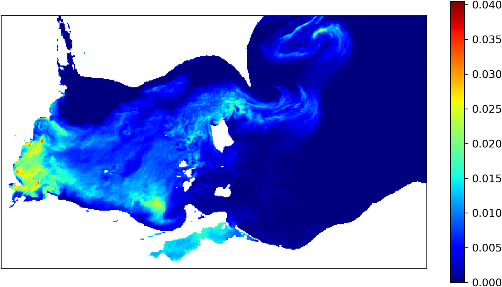
An example cyanobacteria index (CI) image. This image was captured on 3rd Sep 2011. The white region is either land or missing data.
Several images had missing values due to cloud cover over Lake Erie, which makes CI computations from single images unreliable. Therefore, CI was estimated over a period of days, that is, one value of CI over a time period of days (Stumpf et al., 2012) by compositing several images. In this study, 10-day time periods were used to reliably estimate CI values following Stumpf et al. (2012).
To estimate the CyanoHAB intensity during the time period of a composite image, the sum of CI values over all the pixels was computed for the composite image. Fig. 2 shows the values of total CI for each 10-day composite image during the years 2002–2011 and 2016–2020. One may note that the values of total CI reported in Fig. 2 are 16–18 times higher than those reported in Stumpf et al. (2012); this is because full-resolution images were used in this study in contrast to reduced-resolution images used in Stumpf et al. (2012).
Fig. 2.
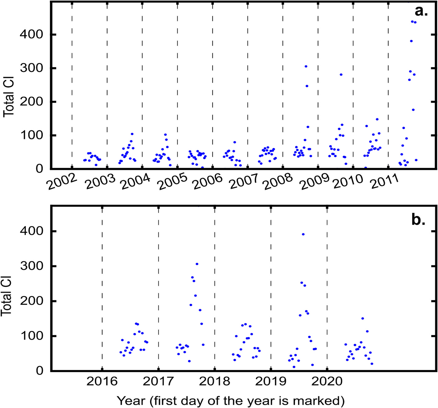
Total CI computed for each of the composite images in Lake Erie during the years 2002–2019 using (a) MERIS and (b) Sentinel-3 observations. The vertical dashed lines signify the first day of the year. The CI values are shown for the months of May-Oct.
2.3. Relationship between satellite-derived cyanobacterial index (CI) and in-situ measures of CyanoHAB intensity
The CI values obtained from the satellite data were regressed against in-situ measured values of phycocyanin (PC) concentration, chlorophyll-a (Chl-a) concentration, and Microcystis biovolume. Pigments Chl-a and PC are found in algae and are often used to quantify the CyanoHAB intensity (Liu et al., 2017; Yan et al., 2018; Ma et al., 2009; Zhu et al., 2022). The concentration of PC allows the determination of bloom intensity. The Chl-a and PC data were available from NOAA field sampling from 2012 to 2018 at 10 locations in western Lake Erie (Burtner et al., 2019). These data may be treated as point scale measurements. Sampling was carried out at irregular time intervals. At some select locations, two samples were collected: one from the surface water layer and the other from the bottom water layer. In addition to PC and Chl-a, in-situ data on Microcystis biovolume (in volume per unit area) were also available from Lake Erie Center (LEC; Bridgeman et al., 2013). These data were available from Apr 2002 to Aug 2016 which overlaps with MERIS remote sensing data. Therefore, CI values obtained from the MERIS satellite corresponding to the pixels coinciding with seven LEC stations were compared with Microcystis biovolume at these stations.
Sentinel-3 satellite data were available from 2016 onwards. The common period between the Sentinel-3 and NOAA field sampling datasets, 2016–2018, was used to derive the relationship between CI and pigment concentrations. CI values of the pixels corresponding to the field sampling location and date were extracted whenever the satellite data were available for the same day and the corresponding pixel was not masked by clouds. Several factors introduce uncertainty in the relationships developed. The size of a pixel is approximately 300m × 300m but chl-a concentration varies at a much smaller scale and CyanoHAB blooms can be very patchy (Kutser, 2004; Reinart and Kutser, 2006). Thus, there exists a spatial scale mismatch between satellite and in-situ data. Also, there exists a mismatch between the timings of CI and pigment concentration measurements. Finally, the CI values may not provide an accurate estimate of CyanoHAB cell count during high wind conditions. CyanoHAB species M. aeruginosa can control its buoyancy and stays on the surface during calm wind conditions. But during high wind conditions, CyanoHABs are distributed throughout the water column; therefore, detection of CyanoHAB intensity using CI values may not be reliable. These factors along with the noise in the satellite data introduce uncertainty in the derived relationship between CI and pigment concentrations. Three outliers were removed from the analysis. These three points had CI values >0.01 but very low PC and Chl-a concentrations which is likely due to the spatial scale mismatch as discussed above.
2.4. Hydro-meteorological and environmental data used as predictor of cyanobacterial index (CI)
Secchi disk depth (SDD) provides a measure of turbidity, and, from the perspective of CyanoHAB growth dynamics, it is a proxy for the depth to which sunlight can penetrate the water column which affects the CyanoHAB growth rate (Huisman and Hulot, 2005). Zolfaghari and Duguay (2016) provided the following formula to estimate SDD:
| (2) |
where and correspond to the 4th and 6th bands in the MERIS data with wavelengths 510 nm and 620 nm, respectively, is the reflectance in the band corresponding to wavelength , and SDD is in meters. In most of the images, a few pixels had negative values of and (Eq. (2)); these pixels were not assigned any value of SDD. Similar to CI images, many of the SDD images had cloud cover which limits their use. Therefore, 10-day composite SDD images were created, similar to 10-day composite CI images (Stumpf et al., 2012).
The wind speed, air temperature, and water level data used in this study were collected from Great Lakes Environmental Research Laboratory (GLERL; https://www.glerl.noaa.gov/metdata/). Among the five stations at which meteorological data were available, the data from the station Erie-cmt (Toledo Channel Marker #2) were used. Solar radiation data were collected from Climate Engine (Huntington et al., 2017). To forecast CyanoHAB cell count at a given time step, minimum, average, and maximum air temperature, minimum, average, and maximum wind speed, water level, and solar radiation during previous time steps were used as predictor variables, among others (Table 1). Wind speed and air temperature data, however, were unavailable for some years between 2002 and 2019. Therefore, wind speed and air temperature data were also collected from Climate Engine to fill in the missing records. Essentially, missing values from GLERL data were imputed by appropriately transforming Climate Engine values as described in Section S1 of supplementary materials (SM).
Table 1.
List of predictor variables for 10-day lead time prediction. Here, refers to time step at which prediction is to be made, , and refer to the lag 1 and lag 2 time steps compared to time step , respectively; 1 time-unit refers to 10 days. The meteorological variables were derived from observed data at 5-minute resolution.
| Variable | Variants of the variables used as predictor |
|---|---|
|
| |
| CI | At time step and |
| Wind speed | Minimum wind speed at time step Average wind speed at time step Maximum wind speed at time step |
| Air temperature | Minimum air temperature at time step and Average air temperature at time step and Maximum air temperature at time step and |
| Total phosphorus (TP) | TP discharged from Maumee, Rasin, Sandusky, and Cuyahoga Rivers averaged over time step TP discharged from Maumee and Raisin Rivers averaged over previous 30 days (i.e., average over , , time steps) Total TP discharged from the four rivers during previous 120 days Legacy (previous 10 years) total TP discharged from the four rivers |
| Total Kjeldahl nitrogen (TKN) | Average TKN discharged from the four rivers during time step Average TKN from Maumee River during previous 60 days Average TKN from Raisin River during previous 30 days Total TKN discharged from the four rivers during previous 120 days |
| Nitrate + nitrite () | Average discharged from the four rivers during time step Average from Maumee and Raisin Rivers during previous 30 days |
| Soluble reactive phosphorus (SRP) | Average SRP discharged from the four rivers during time step Average SRP from Maumee and Raisin Rivers during previous 30 days |
| Total suspended solids (TSS) | Average TSS discharged from the four rivers during time step Average TSS from Maumee and Raisin Rivers during previous 30 days |
| Average streamflow | Average streamflow discharged from the four rivers during time step Average streamflow discharged from Maumee and Raisin Rivers during previous 30 days |
| Ration of TKN to TP | Ratio of TKN to TP in the four rivers during time step |
| Ration of TKN to () | Ratio of TKN to () in the four rivers during time step |
| Average solar radiation | At time step (average over previous 10 days) 30-day average of solar radiation between time steps to |
| Average water level | At time step and |
| Secchi depth | At time step |
| Observation time step of the year | Position of 10-day composite time-period, for which CI is to be forecasted, in the complete sequence of the year. For example, period May 1 to May 10 is at 1st position, so it was assigned a value of 1 for this variable. Similarly, next 10-day period (May 11 to May 20) was assigned a value of 2 for this predictor. |
The residence time of water in the lake also affects the growth rate of cyanobacteria: a longer residence time allows for more growth. To get an estimate of the residence time of water in Lake Erie, daily streamflows of the Maumee, Raisin, Sandusky, and Cuyahoga Rivers were used as predictor variables. To forecast the CI value at the current time step, average daily discharges from each of the four rivers during the previous time steps were used as predictor variables. Hereinafter, these variables are referred to as ‘average daily streamflow’.
Phosphorus and nitrogen nutrients available in the lake are among the most important factors controlling the CyanoHAB growth rate (Chaffin et al., 2013). The dominant sources of nutrients in the lake are four rivers (Baker et al., 2014; Stow et al., 2015): Maumee, Raisin, Sandusky, and Cuyahoga. While the Detroit River is also a major river flowing into the lake, hardly any data are available for this river, and hence not considered in the analysis. These rivers drain large agriculture-intensive watersheds. Nutrient concentration data in these rivers were obtained from Heidelberg Tributary Loading Program (HTLP; NCWQR, 2022). Concentration data, available at sub-daily timescale, were converted to daily timescale by dividing the daily load in the river by daily streamflow.
In this study, average TP and TKN loads discharged in the lake in preceding time steps along with the ratio of TKN to TP were also used as predictors. In addition to TP and TKN, nitrate + nitrite (), soluble reactive phosphorus (SRP), total suspended solids (TSS), and the ratio of TKN to at preceding time steps were used as predictor variables. Also, TP load in the preceding 120 days (TP 120, i.e., aggregated over 120 days) and TKN load in the preceding 120 days (TKN 120), were used as predictor variables in this study. Another source of TP to the water column could be the lakebed which is referred to as ‘Legacy TP’. Since it is not possible to readily estimate legacy TP, TP discharged into the lake during the preceding 10 years (Ho and Michalak, 2017) from the four rivers were also used as predictor variables. The following variables will be referred to as ‘integrated nutrient variables’: Legacy TP, TP 120, and TKN 120.
The growth dynamics of CyanoHAB cell count have two phases: a growth phase and a mortality phase. It is therefore plausible that given the same values of all the predictor variables, the value of CI at the next time step will be different in the growth and mortality phases. In Lake Erie, the growth phase occurs approximately during the months of May to August and the mortality phase occurs during the months of September to Oct. Thus, the information about the time steps at which the prediction is being made can help predict the CyanoHAB cell count. Therefore, a predictor labeled ‘observation time step’ was also used in this work. Each 10-day time period, used for image composition, in a year was assigned an integer value between 1 and 18 according to their position in the time series. For example, the period May 1 to May 10 was assigned a value of 1, the next period, May 11 to May 20, was assigned a value of 2, and so on up to Oct 22 to Oct 31.
2.5. Predictor variables with lags of more than one time step
Predictor variables at larger than one time lag (averaged over the previous 10 days) may be relevant in explaining the variations in CI. A correlation analysis between the time series of CI and other hydro-meteorological and nutrient variables was carried out to identify important predictor variables at different lags. To understand how these multiple time lag variables help explain the variation in CI, two sets of ML models were developed to forecast CI: (1) Using variables with time lag 1 only, and (2) Using variables with multiple time lags along with lag 1 variables.
2.6. Machine learning (ML) models
An ML model creates a mapping between two sets of variables referred to as predictor and response variables. Predictor variables are provided as input to the model and response variable is the model output. Models were developed to forecast CI at one time step (10 days), two time steps (20 days), and three time steps (30 days) lead time. For the 10-, 20-, and 30-day lead time prediction, the predictor variables at time steps , and , respectively, were used to forecast CI at time step . For example, for the 10-day lead time forecast (future 10-day time window), CI at the time step was used as a predictor where refers to the 10-day window for which prediction is required. Similarly, for 20-day lead time forecast (future 20-day time window), CI at the time step was used as a predictor. Other predictor variables were also used as shown in Table 1. For example, the average of solar radiation between time steps and was used as a predictor variable to forecast CI at time step .
Three ML algorithms were used in this study: LASSO (Least Absolute Shrinkage and Selection Operator; Abu-Mostafa et al., 2012), ANN (Artificial Neural Network; Haykin, 2009), and RF (Random Forest; Breiman, 2001). Also, an ensemble average (EA) of the three models was used as the fourth algorithm. A brief description of the four algorithms follows:
LASSO: Let denote the matrix containing predictor variables where each row contains one instance, and each column contains one predictor variable. Let denote the vector of the logarithm of response variables, that is, logarithm of CI at time step . A linear model
| (3) |
was hypothesized as a reasonable relationship between the logarithm of CI and predictor variables. In Eq. (3), denotes the coefficient vector, denotes the number of predictor variables, and denotes the error-term. Because different predictors have different units and ranges, each predictor in was mean-centered and scaled by their corresponding standard deviations. The vector of coefficients and were estimated by minimizing the objective function
| (4) |
where the first term on the right-hand side denotes the sum-of-square errors, the second term on the right-hand side denotes the regularization term, denotes the regularization parameter, and the superscript denotes the matrix transpose. The regularization term denotes the norm of which is minimized to eliminate the unimportant predictor variables from the analysis. Here, denotes the absolute value of . Operationally, regularization refers to the adjustment of the weight vector to avoid overfitting during the training phase. One of the reasons for overfitting is noise in the predictor variables and/or response variable. The magnitude of the weight of a predictor variable determines the effect of the noise on the estimated response. The smaller the weight, the smaller the effect of noise on the estimated response. The parameter controls the amount of regularization applied. Setting to a very small value may result in overfitting (the model may fit the noise) and setting to a very large value will result in a poor training (the model will not fit data). In both cases, the performance of the models will be poor. Therefore, the regularization parameter needs to be tuned to an optimal value. The candidate values of ranged from 0 to where is the value above which weight vector becomes zero. The method to determine the optimal value of is described in Section S2 (SM).
Random forest (RF): One of the limitations of the LASSO algorithm is that it is limited to a linear relationship between the predictor and response variables. Therefore, the RF algorithm was also used in this study as it can identify non-linear relationships between predictor and response variables. The RF algorithm is based on the idea of regression trees (Friedman et al., 2001). The regression tree algorithm divides the space of predictor variables into (contiguous) subregions, and in each subregion, the response variable is approximated by a simple function. Division of predictor space into S subregions divides the training set into smaller subsets depending upon the value of corresponding predictor variables. In each subregion, a simple relationship between predictor and response variables is estimated.
In RF, several decision trees are created instead of just one, and the final prediction is the average of predictions made by all the decision trees. Thus, the RF algorithm avoids over-fitting to the training data. Each decision tree is created by using a bootstrap sample of training data. Three RF parameters were tuned: the number of decision trees, the minimum number of samples in the leaf node, and the number of predictor variables to be used at each node for dividing the predictor space. The method of finding optimal values of these parameters is provided in Section S2 (SM).
Artificial neural network (ANN): The ANN algorithm is the third method used in this study to establish a non-linear relationship between predictor and response variables. It is a very well-known algorithm, and the interested reader is referred to Haykin (2009) for details. Here, we briefly describe the main ideas. The basic architecture of ANN includes multiple layers in sequence. Each layer consists of a different number of non-linear processing units which are referred to as neurons. The first layer is referred to as the input layer because predictor variables are fed to this layer as inputs; the number of neurons in the input layer is equal to the number of predictor variables . The last layer is referred to as the output layer as it produces the required response variable estimate; the number of neurons in this layer is equal to the number of response variables which is 1 in this study. The layers between the input and output layers are referred to as hidden layers. A neural network can capture non-linearities in the relationship between predictor and response relationship because of non-linear processing by neurons. The number of hidden layers and the number of neurons in each of the hidden layers are tuning parameters. In this study, 3 hidden layers were used with 4, 3, and 2 neurons in the first, second, and third hidden layers, respectively. This specific configuration was determined based on experimentation with different trial configurations.
An ANN processes the information contained in the inputs sequentially from the input to the output layer: the outputs of a layer become the inputs to the next layer. The neurons in each layer apply a non-linear function to weighted sums of the inputs; the weighted sums are different for different neurons. The weights are parameters of the network which are optimized using the backpropagation algorithm to minimize MSE between the estimated and observed values of the response variable. The backpropagation algorithm is implemented iteratively, and each iteration is referred to as an epoch. With each epoch, the training MSE decreases. If the number of epochs is kept small, the network remains undertrained; if the number of epochs is large, the network overfits the data. In both cases, the prediction capability of the trained models will be poor on the test set. Therefore, the number of epochs is a tuning parameter. The method of finding the optimal number of epochs is provided in Section S2 (SM).
The parameters of an ANN may converge to very different sets of values depending on the initial values of the parameters, which may result in different estimates of the response variable. In this study, the average of 20 ANNs initialized with different parameter values was taken as the estimate of the response variable.
Ensemble average of models (EA): The three ML models discussed above are based upon different ideas and yield different response variable estimates for a given predictor vector. Therefore, the average of the estimates of the three models was taken as the ensemble-average model. In this study, MSE-weighted average was taken. In the MSE-weighted average, the prediction was made as:
| (5) |
where is the cross validation MSE of method obtained during the parameter tuning (Section S2 in SM).
2.7. Training and testing
After removing the samples with >10% cloud cover in the composite image, a total of 177 observations were identified. The samples with cloud cover >10 % were removed because cloud cover may result in an underestimation of the CI values. The threshold of 10 % was selected so that a significant proportion of the samples were retained for developing ML models.
To develop an ML model, data are typically divided into training and testing sets. The training set is used to estimate the model parameters, while the testing set is used to evaluate the trained model’s performance on unseen data. Because of limited data, LASSO, RF, and ANN were trained and tested in two ways (Friedman et al., 2001): bootstrap sampling (BS) and leave-one-out cross-validation (LOOCV). In the BS scheme, 1000 training and test set pairs were created by randomly dividing the dataset. Each training set had 107 samples, and the test set had the remaining 70 samples. LASSO, RF, and ANN models were trained and tested for each pair. In the LOOCV scheme, as many realizations of the training and test set pairs were created as the total number of samples in the dataset (i.e., 177). Each pair contained one sample in the test set and the rest of the samples in the training set. The realizations of the pairs of training and test sets were created such that each sample could be in the test set in exactly one of the realizations. The performance of the algorithms was assessed using the coefficient of determination , computed as the square of the correlation coefficient.
2.8. Importance of predictor variables
The importance of different variables in forecasting CyanoHAB cell count was determined using the LASSO and RF algorithms. Using the LASSO regression, the importance of a variable in forecasting the total CI was determined as proportional to the absolute value of the regression coefficient (w) of the predictor. A thousand BS realizations yielded 1000 regression coefficients for a predictor variable which were used to determine first whether the coefficient of a predictor variable is statistically different from zero or not, then determine its importance based on the absolute value of the 1000 coefficients.
In RF, the importance of a predictor was determined by computing the relative increase in MSE by randomly permuting the variable. If a predictor variable is important, its importance value will be positive and substantially greater than zero. When the sample size is small compared to the number of predictor variables, the importance of the predictor variable may come out to be a negative number, indicating the data corresponding to the predictor variable are noisy and do not contribute to the forecasting of the response variable. Similar to LASSO, 1000 BS realizations yielded 1000 values of the importance of a predictor variable using RF.
A non-parametric statistical significance test was carried out to determine if the regression coefficients obtained by the LASSO and the importance values obtained by the RF were statistically different from 0. The p-values were computed for the regression coefficients and importance values as follows. In the case of importance values obtained by the RF, the p-value was computed as the probability that the importance value of the predictor variable was less than or equal to 0 using the 1000 importance values obtained by the BS scheme. In the case of the LASSO regression coefficients, two probabilities were computed: (1) the regression coefficient of a predictor variable was >0 and (2) the regression coefficient was <0. The minimum of the two probabilities was computed as equal to the p-value. The predictor variables for which the corresponding regression coefficients or importance values had their p-value <0.05 were considered statistically significant in forecasting the total CI. A higher magnitude of regression coefficients and/or importance value of a variable indicate higher importance of the variable.
2.9. Predictive uncertainty analysis
For the practical applications of the models developed in this study, an estimate of predictive uncertainty is also required. To estimate the predictive uncertainty, skewed generalized Gaussian distribution SGGD (Fernández and Steel, 1998) was fitted to the residuals obtained from the various models. The general form of univariate SGGD is:
| (6) |
where is the skew parameter, is the indicator function which is equal to 1 when and 0, otherwise, and is the power exponential distribution (Box and Tiao, 1973) with scale parameter and shape parameter ,
| (7) |
where denotes the gamma function. The parameters of the distribution were estimated by maximizing the log likelihood of the residuals. The goodness of fit of the fitted statistical distribution was assessed using quantile-quantile (QQ) plot. Note that at , the distribution becomes equal to and by setting , and the distribution becomes zero-mean Gaussian. Once the parameters of the error model were estimated, 95 % prediction intervals were computed by drawing random samples from the error model. Note that the residuals were assumed statistically independent of each other.
3. Results and discussions
3.1. Relationship between CI and CyanoHAB
NOAA in-situ samples were collected from both the surface and bottom water layers. So, two relationships were derived: (1) Between CI and surface layer in-situ pigment concentrations, and (2) Between CI and bottom layer in-situ pigment concentration. Even though satellite-derived CI values only reflect the surface layer pigment concentrations, CI values may be correlated to bottom pigment concentration due to the correlation between surface and bottom concentrations. Fig. 3 shows the relationships of CI with Chl-a and PC concentrations. The relationships of CI with PC concentrations had and 0.53 for surface and bottom in-situ samples, respectively. Similarly, the relationships between CI and surface/bottom water layer Chl-a concentration had . Overall, these results give us confidence in using CI as a proxy for CyanoHAB cell count in Lake Erie. Moreover, these relationships can be used to convert CI into PC and Chl-a concentrations which can help water managers understand the severity of an algal bloom. Table 2 lists these relationships.
Fig. 3.
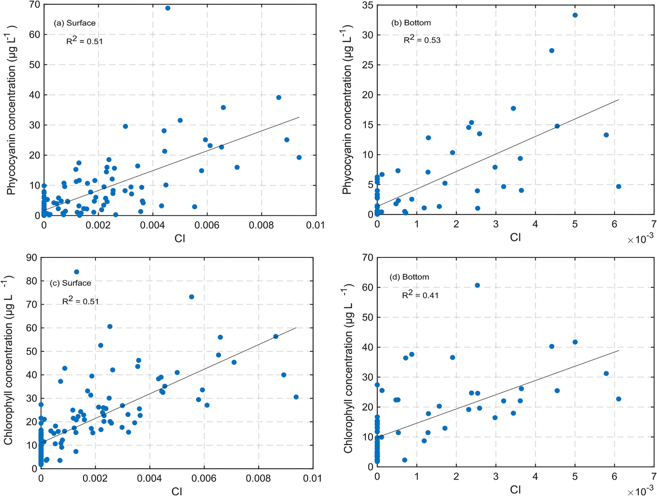
Variation of phycocyanin and chlorophyll concentrations with CI. The black line is the best fit linear line, plots on the left for surface samples, and the plots on the right are for bottom (near the lakebed) samples.
Table 2.
Relationship between CyanoHAB pigment concentrations and CI values.
| Response variable () | Equation | p-Values (intercept, slope) | |
|---|---|---|---|
|
| |||
| Surface phycocyanin concentration (μg L−1) | = 1.72+3290.95 | 0.51 | (0.011,1.93 × 10−23) |
| Bottom phycocyanin concentration (μg L−1) | = 1.33 + 2925.63 | 0.53 | (0.031,5.49 × 10−13) |
| Surface chlorophyll concentration (μg L−1) | = 10.98 + 5235.12 | 0.51 | (6.4 × 10−19,2.29 × 10−23) |
| Bottom chlorophyll concentration (μg L−1) | = 9.85 + 4755.66 | 0.41 | (2.2 × 10−11,1.19 × 10−9) |
Water managers also need estimates of the mass of these pigments per unit area of the lake. The quantity ‘mass per unit area’ will be referred to as areal concentration in what follows. The water column was divided into three layers: an upper layer of length , a middle layer of length , and a lower layer of length . The observations of concentrations are available at the lower end of the upper and middle layers. Let these concentrations be denoted by and , respectively. Further assuming that concentrations within the upper and lower layer are constant (equal to and , respectively) and that the concentration in the middle layer changes linearly with depth, the average concentration in the water column comes out to be
| (8) |
and the mass per unit area comes out to be . A direct relationship between CI and pigment areal concentrations could not be identified, because there were only a few days when both surface and bottom pigment concentrations were available simultaneously with CI values. Fortunately, there exists a strong correlation between the areal concentrations and surface layer volume concentrations (Fig. 4). Fig. 4 shows that areal concentrations can be computed accurately using the volume concentration in the surface layer for both the pigments, PC and Chl-a. Table 3 lists the relevant relationships.
Fig. 4.
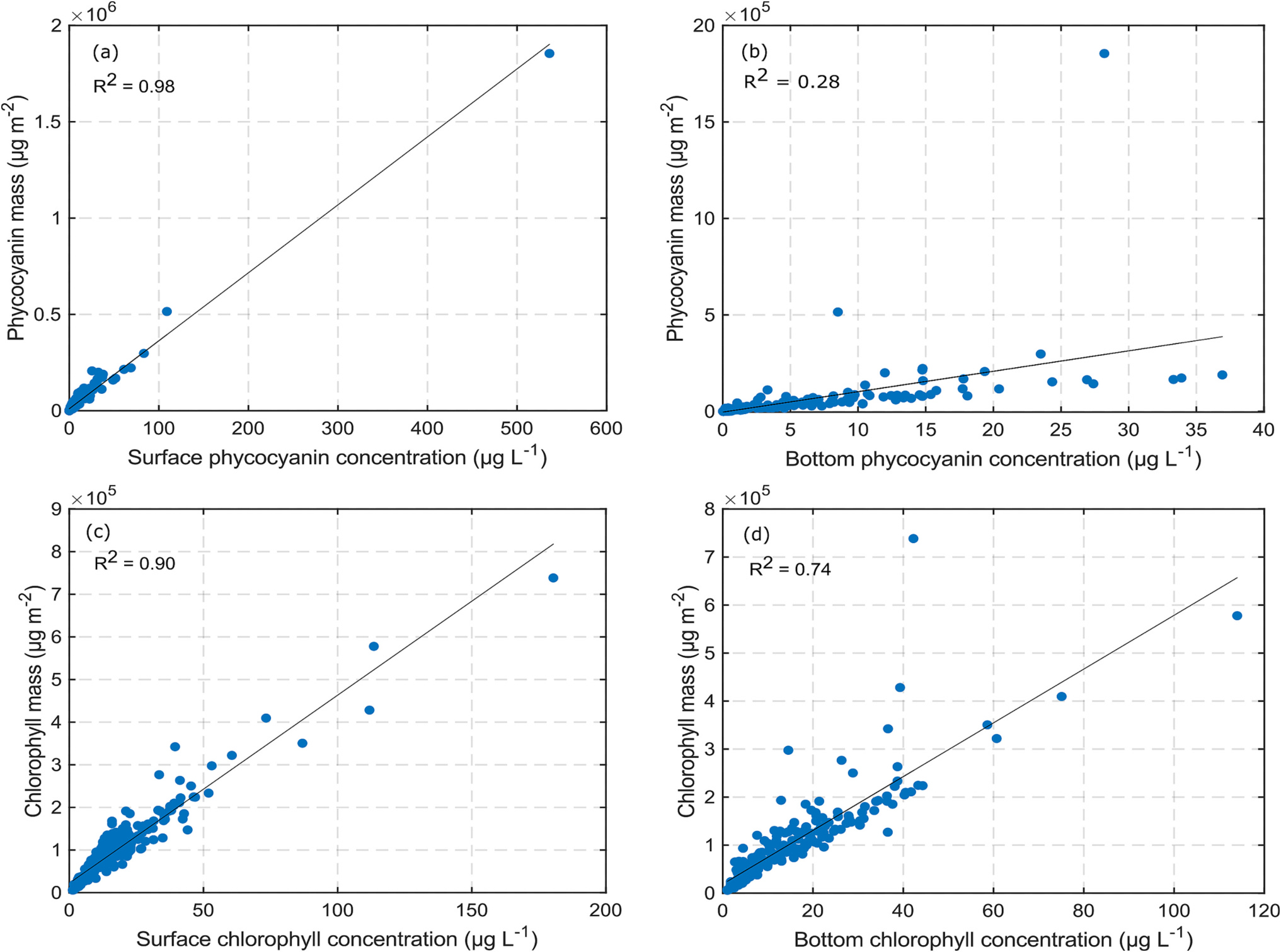
Variation of phycocyanin (top panels) and Chlorophyll (bottom panels) concentrations (mass per unit area) with respective surface (left panels) and bottom (right panels) concentrations. The black line is the best fit linear line.
Table 3.
Relationship between CyanoHAB pigment areal and volume concentrations.
| Response variable () | Predictor variable () | Equation | p-Values (intercept, slope) | |
|---|---|---|---|---|
|
| ||||
| Phycocyanin areal concentration (μg m−2) | Surface phycocyanin concentration (μg L−1) | 0.98 | (4.04 × 10−12,0) | |
| Bottom phycocyanin concentration (μg L−1) | 0.28 | (0.71, 2.91 × 10⁻¹⁶) | ||
| Chlorophyll areal concentration (μg m−2) | Surface Chlorophyll concentration (μg L−1) | 0.91 | (2.421 × 10−15,0) | |
| Bottom Chlorophyll concentration (μg L−1) | 0.74 | (8.56 × 10−5,0) | ||
The relationships in Table 2 can be used to convert CI into pigment volume concentration, and the relationships in Table 3 can be used to convert pigment volume concentrations to pigment areal concentrations. Thus, the total CI value over the lake can be converted to the total mass of the CyanoHAB pigments in the lake.
Fig. 5a and Table 4 show the relationship between CI and Microcystis biovolume using the data from all the LEC stations. The relationship had but had a statistically significant slope with p-value equal to 3.8 × 10⁻⁵.
Fig. 5.
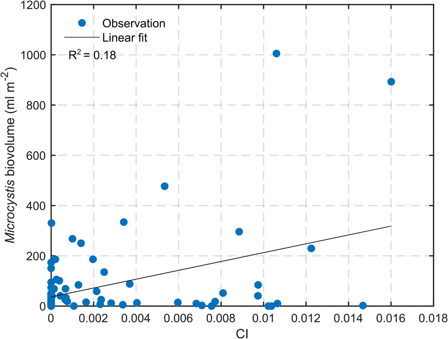
Variation of Microcystis biovolume with CI along with best-fit line.
Table 4.
Relationship between CI and Microcystis biovolume.
| Response variable () | Equation | p-Values (intercept, slope) | |
|---|---|---|---|
|
| |||
| Microcystis biovolume (ml m−2) with MB stations | = 36.59 + 1760.62 | 0.18 | (0.047,3.8 × 10−5) |
The analysis presented above suggests that there exists a relationship between CI and various in-situ measures of CyanoHAB presence in the lake. But the exact relation could not be derived because of various uncertainties mentioned above and there was a significant scatter around these relationships. More in-situ data are required to reduce uncertainty in the relationship between satellite-derived CI and CyanoHAB cell count. In what follows, the terms ‘CI’, CyanoHAB cell count, and CyanoHAB intensity are used interchangeably.
3.2. Correlation of CI with multi-lag variables
Fig. 6 shows the correlations of hydro-meteorological variables with 10-day composite CI at different time lags. Air temperature (minimum, maximum, and average) had strong correlations with CI at all the lags, with maximum correlation at lag 3 (i.e., 30 days). Therefore, air temperature at lag 3 was used as a predictor variable in this study. Wind speed was not correlated with CI at any lag except the minimum wind speed which was negatively correlated at lag 1. Solar radiation was not correlated at lags 1, 2, or 3, but had high correlations with CI at lags 4, 5, and 6. In this study, the average of solar radiation at lags 4, 5, and 6 was used as a predictor variable. The water level had strong positive correlations at all the lags with the highest correlation at lag 6. In this study, the water level at lag 6 was used as a predictor variable. CI had strong autocorrelation at lags 1, 2, 3, 4, and 5. In this study, CI at lag 2 was used as a predictor variable along with CI at lag 1.
Fig. 6.
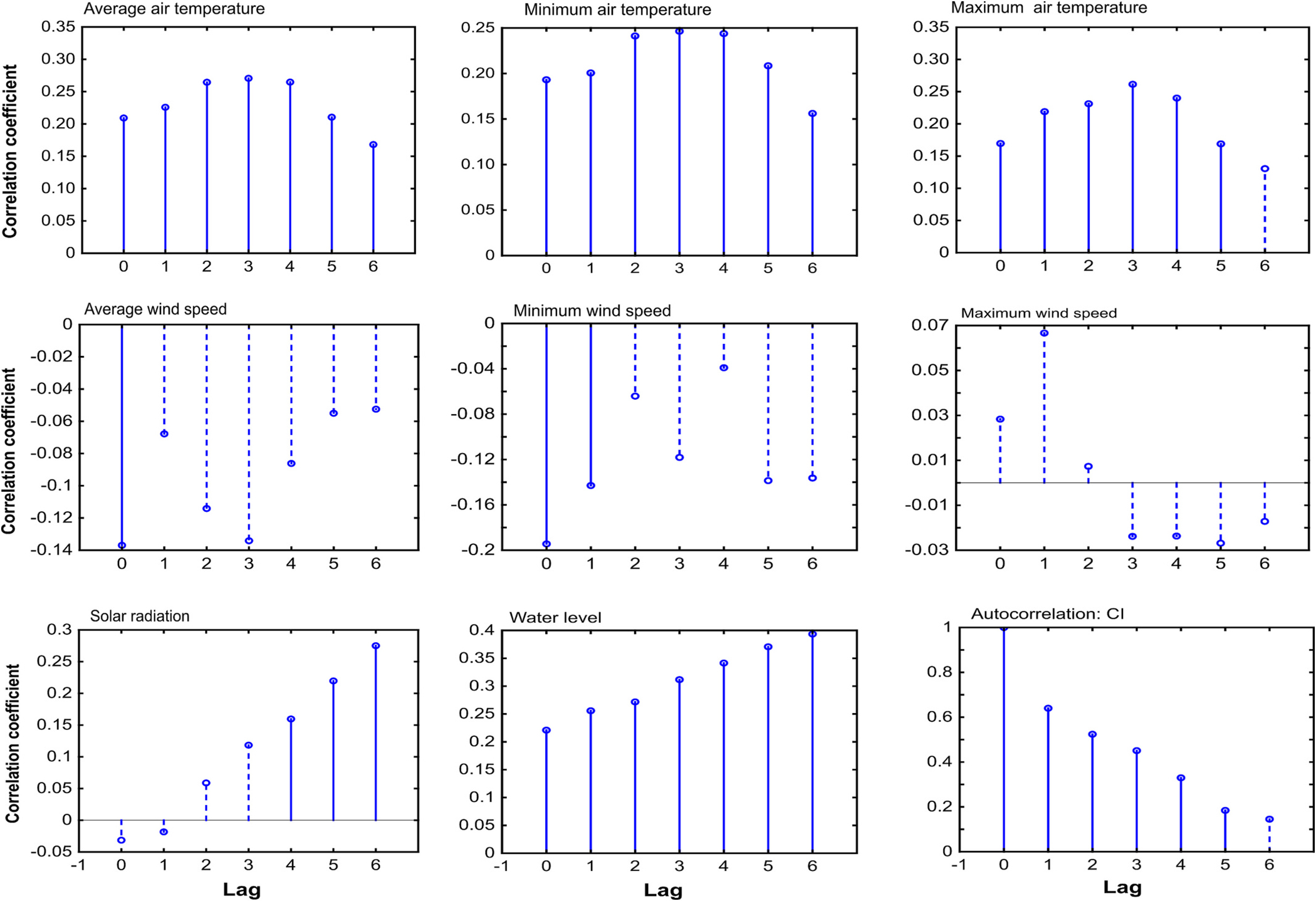
Correlation of meteorological variables with CI and auto-correlation of CI at different time-lags where one time-lag corresponds to 10 days. Solid and dashed bars show statistically significant and insignificant correlations at 5 % significance level, respectively.
Fig. 7 shows the correlations of the 10-day average nutrient loading time series with the 10-day composite CI time series at different lags. TP was not correlated with CI at any lag. TKN from Raisin River was positively correlated with CI at lags 1, 2, 3, and 4. from Maumee and Raisin Rivers had moderate negative correlations with CI at lags 1 and 2, and at lags 1,2, and 3, respectively. SRP from Maumee River had a negative correlation with CI at lag 1. TSS discharged from any of the four rivers were not correlated with CI at any time lag (not shown) except the TSS discharged from Raisin River at lag 3.
Fig. 7.
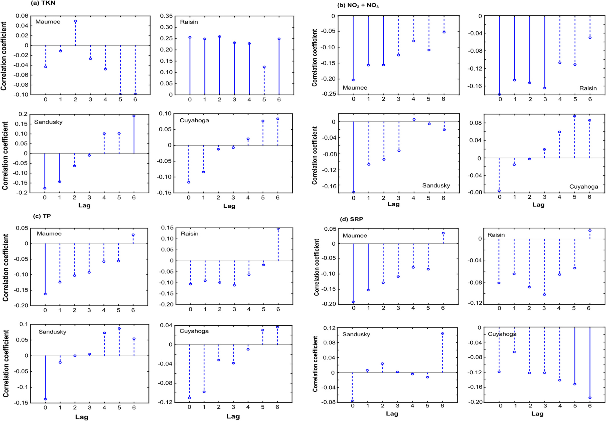
Correlation between (a) total Kjeldahl Nitrogen (TKN), (b) Nitrite and Nitrate (), (c) total phosphorus (TP), and (d) soluble reactive phosphorus (SRP) discharged from the four rivers and CI at different time-lags where one time-lag corresponds to 10 days. Solid and dashed bars show statistically significant and insignificant correlations at 5 % significance level.
Fig. 8 shows the correlations of CI with nutrients and streamflow discharged from the four rivers aggregated and averaged over the previous 30, 40, 50, and 60 days. All the discharges (nutrients and streamflow) from Maumee River averaged over the previous 30, 40, 50, and 60 days had a negative correlation with CI. The negative correlation between TP and CI is surprising. Among various discharges from Raisin River, TP, , and TSS daily loadings, and rivers discharge rates averaged over the time periods had negative correlations with CI. But TKN load discharge from Raisin River averaged over the time periods had strong positive correlations with CI. Based on these correlation plots, the following variables were used as predictor variables: (1) Daily TP discharged from Maumee and Raisin Rivers averaged over the previous 30 days, (2) Daily TKN discharged from Maumee and Raisin Rivers averaged over previous 60 and 30 days, respectively, (3) Daily discharged from Maumee and Raisin Rivers averaged over previous 30 days, (4) Daily SRP discharged from Maumee River averaged over previous 30 days, (5) Daily TSS discharged from Maumee and Raisin Rivers averaged over previous 30 days, and (6) Daily streamflows from Maumee and Raisin Rivers averaged over previous 30 days.
Fig. 8.
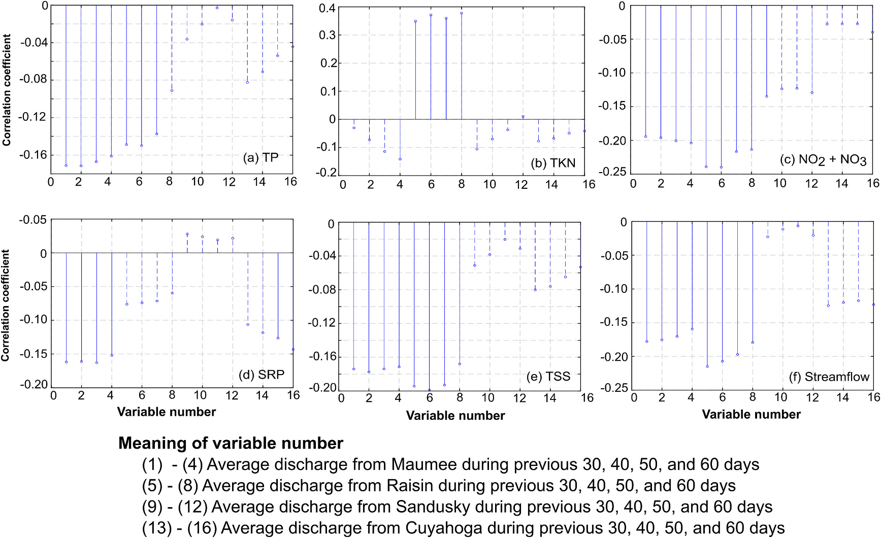
Correlation of the total CI with daily average nutrient loads and streamflow discharged from the four River during the previous 30, 40, 50, and 60 days. Solid and dashed bars show statistically significant and insignificant correlations at 5 % significance level. TP = Total phosphorus, TKN = Total Kjeldahl nitrogen, , SRP = Soluble reactive phosphorus, TSS = Total suspended solids. All nutrients are in kg/day unit and streamflow is in m3/s units.
3.3. Analysis with predictor variables at one time lag
Fig. 9 shows boxplots of the coefficients of determination () of the logarithm of total CI obtained by using the LASSO, ANN, RF, and EA models for 10-, 20- and 30-day lead time forecasting, for 1000 BS test sets. This figure also shows the results obtained using the multi-lag predictor variables, these results will be discussed in the next section. In all the scenarios, the RF was better than the LASSO with substantial differences for the 20- and 30-day lead time forecasts. The ANN performed slightly worse than the LASSO for the 10-day lead time forecasts, but better than LASSO for the 20- and 30-day lead time forecasts. The EA and the RF performed similarly for 10-day and 20-day lead time forecast. The mean values obtained by the LASSO, ANN, RF, and EA for 10-day lead time forecast were 0.54, 0.52, 0.59, and 0.59, respectively. The mean values obtained by the LASSO, ANN, RF, and EA for 20-day lead time forecast were 0.44, 0.51, 0.56, and 0.54, respectively. The mean values obtained by the LASSO, ANN, RF, and EA for 30-day lead time forecast were 0.37, 0.50, 0.53, and 0.43, respectively.
Fig. 9.
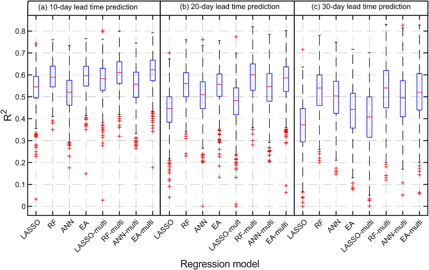
Box plots of coefficient of determination obtained by using LASSO regression, random forest (RF), artificial neural network (ANN), and ensemble average (EA) for (a) 10-day lead time prediction, (b) 20-day lead time prediction, and (c) 30-day lead time prediction of log-CI. These results were obtained using bootstrap sampling (BS) scheme on the test set.
Fig. 10 shows the observed and forecasted logarithm of total CI values for the test set using the LOOCV scheme. The RF outperformed the LASSO and the ANN for all three lead time forecasts. The EA and the RF performed similarly. For all three lead time forecasts, the large CI values were poorly forecasted and often underestimated across all the models. Due to fewer samples with large CI values, the ML algorithms could not approximate the relationship between the predictor and response variables for the high CI values.
Fig. 10.
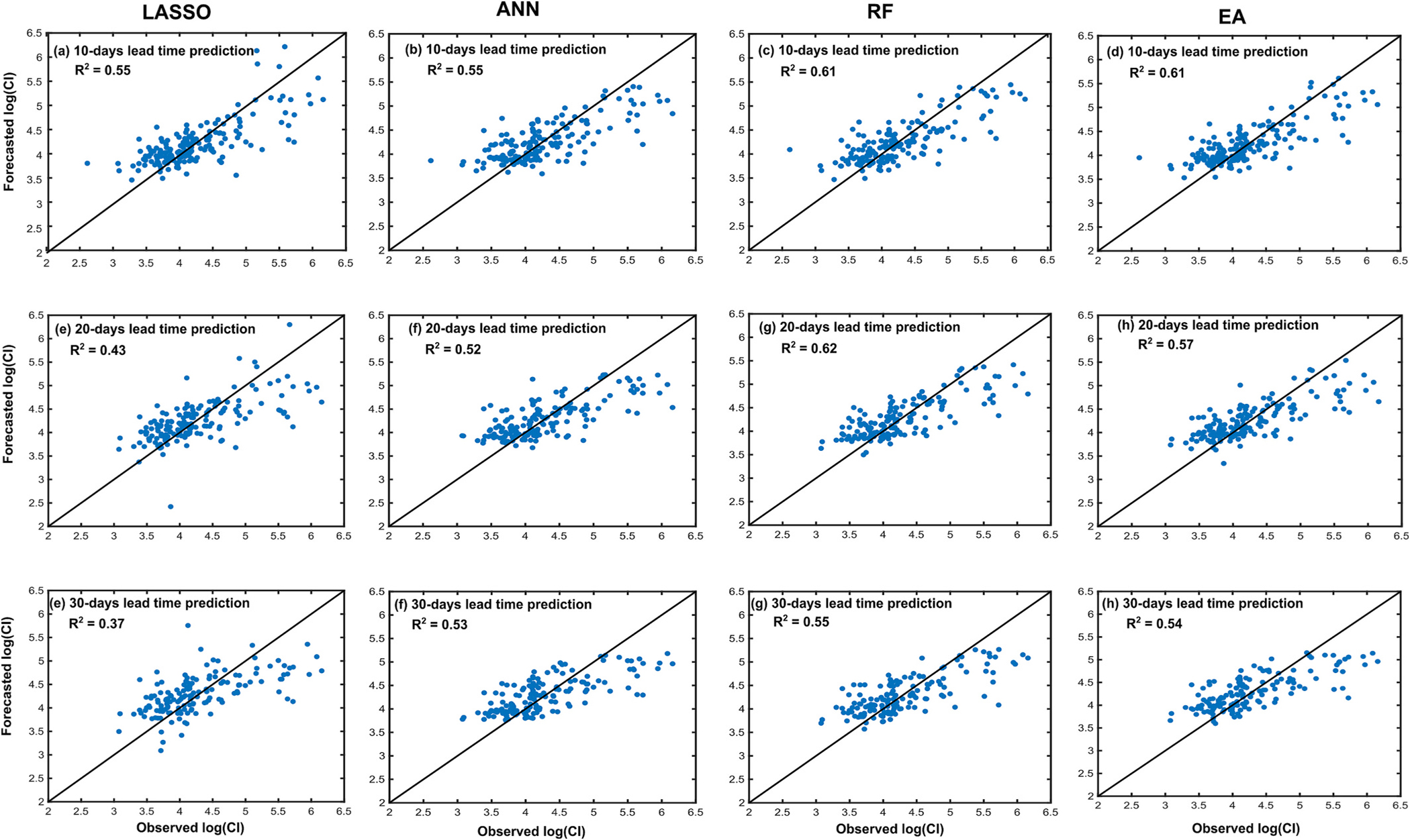
Observed and forecasted logarithm of CI excluding multi-lagged predictor variables using LASSO (first column), ANN (second column), random forest (RF; third column), and Ensemble Average (EA, fourth column). These results were obtained using leave-one-out cross-validation (LOOCV) scheme on the test set.
Table 5 lists the values obtained by the LOOCV scheme along with the fitted parameters of the SGGD to the corresponding residuals. For almost all the models, the shape parameter was significantly >0 but the skew parameter was close to 1, implying that a symmetric but heavy-tailed distribution was required to model the statistical structure of residuals. This information can be used to estimate the predictive uncertainty in the modeled CI values. The predictive uncertainty plots corresponding to EA models are shown in Fig. 11 which shows the 95 % prediction interval obtained from analysis of the residuals. The uncertainty bounds obtained were very wide. The statistical structure of the residuals is dependent upon the model and the data used to train the model.
Table 5.
LOOCV scheme. Coefficient of determination () for test set and error model parameters obtained for different models. The parameter denotes standard deviation, denotes shape parameter, and denotes the skew parameter. The parameter was derived from the scale parameter following Box and Tiao (1973).
| Model | Coefficient of determination () | Error model parameters (, , ) |
|---|---|---|
|
| ||
| 10-Day lead time forecast | ||
| Without multiple lag predictor variables | ||
| LASSO | 0.55 | (0.43, 0.60, 1.02) |
| ANN | 0.55 | (0.44, 0.49, 1.01) |
| RF | 0.61 | (0.41, 0.49, 1.01) |
| EA | 0.61 | (0.41, 0.38, 1.02) |
| With multiple lag predictor variables | ||
| LASSO | 0.60 | (0.40, 0.54, 1.03) |
| ANN | 0.59 | (0.42, 0.44, 1.02) |
| RF | 0.62 | (0.40, 0.19, 1.03) |
| EA | 0.64 | (0.39, 0.52, 1.03) |
| 20-Day lead time forecast | ||
| Without multiple lag predictor variables | ||
| LASSO | 0.43 | (0.48, 0.57, 1.05) |
| ANN | 0.52 | (0.45, 0.31, 1.02) |
| RF | 0.62 | (0.41, 0.30, 1.04) |
| EA | 0.57 | (0.43, 0.35, 1.04) |
| With multiple lag predictor variables | ||
| LASSO | 0.43 | (0.48, 0.57, 1.06) |
| ANN | 0.54 | (0.45, 0.36, 1.02) |
| RF | 0.64 | (0.41, 0.41, 1.02) |
| EA | 0.59 | (0.43, 0.46, 1.04) |
| 30-Day lead time forecast | ||
| Without multiple lag predictor variables | ||
| LASSO | 0.37 | (0.51, 0.14, 1.02) |
| ANN | 0.53 | (0.46, 0.04, 1.05) |
| RF | 0.55 | (0.44, 0.23, 1.02) |
| EA | 0.54 | (0.45, 0.10, 1.04) |
| With multiple lag predictor variables | ||
| LASSO | 0.38 | (0.52, 0.28, 1.03) |
| ANN | 0.55 | (0.46, 0.05, 1.03) |
| RF | 0.57 | (0.45, 0.25, 1.03) |
| EA | 0.55 | (0.46, 0.15, 1.04) |
Fig. 11.
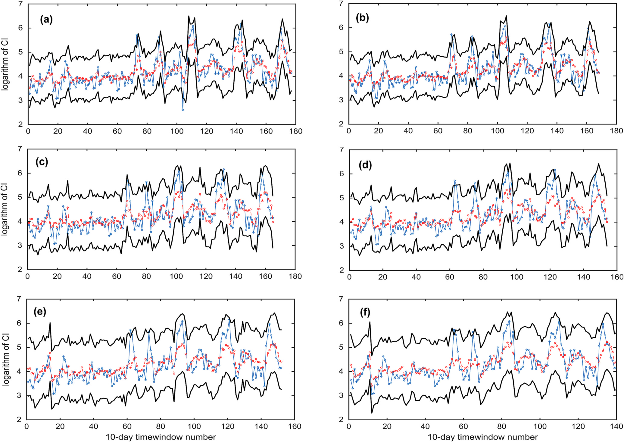
Ensemble Average (EA) models. LOOCV scheme. The observed (blue solid line), forecasted (red dash line), and 95 % prediction interval (black solid line). The subplots (a, b) correspond to 10-day lead time prediction, subplots (c, d) correspond to 20-day lead time prediction, and subplots (e, f) correspond to 30-day lead time prediction. The subplots on the left- and right-hand size correspond to without (Section 3.3) and with (Section 3.4) multiple time-lag variables, respectively.
Figs. 12–14 show the distributions of the importance of different predictor variables obtained by using the LASSO and RF for the 10-, 20- and 30-day lead time predictions without multiple time-lag variables, respectively. These results will be discussed next.
Fig. 12.
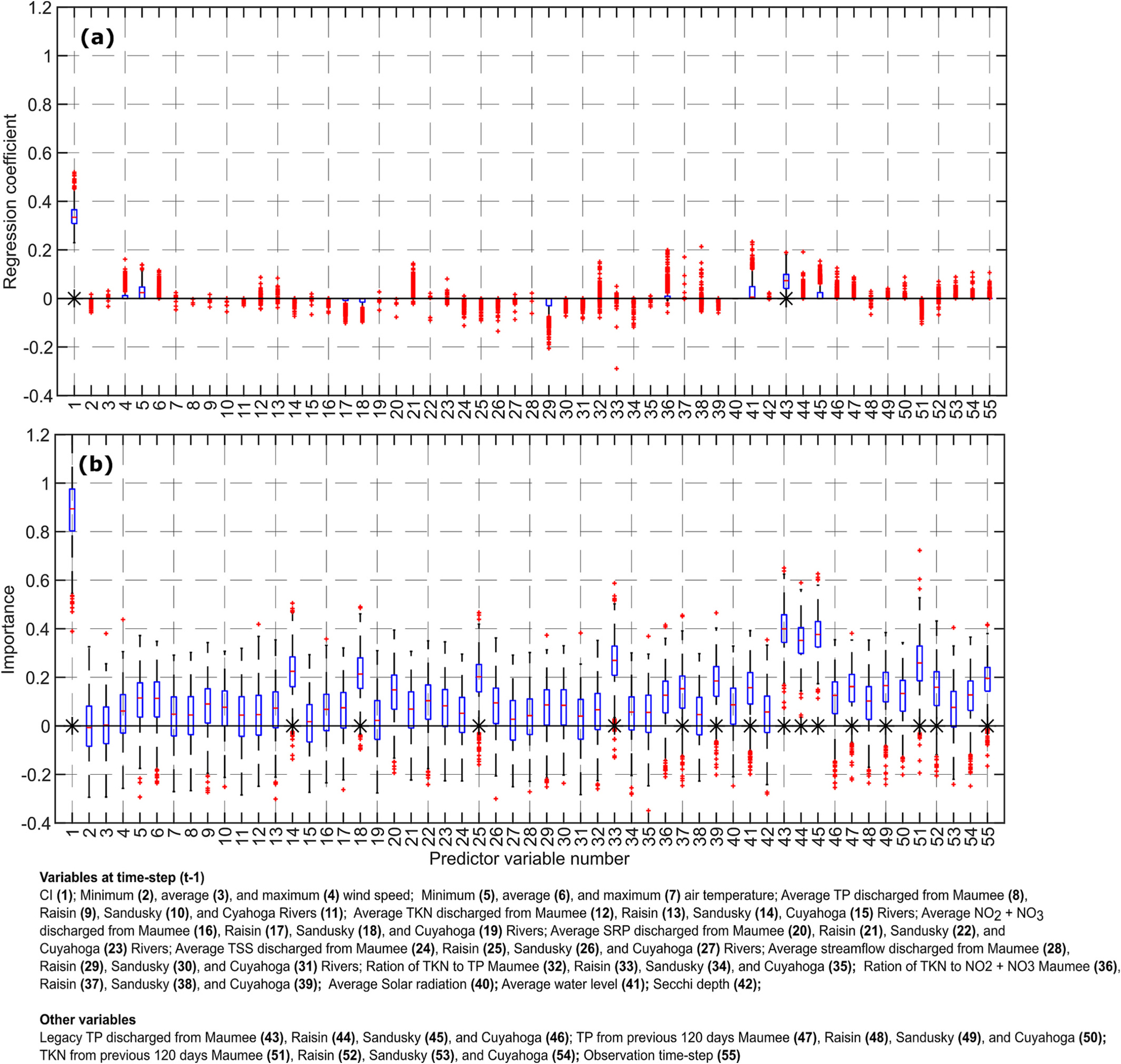
10-Day lead time forecast. Boxplots of the importance of the predictor variables obtained by using LASSO (top), and random forest (RF, bottom). These results were obtained using bootstrap sampling (BS) scheme. The symbol ‘*’ indicates that the variable was statistically significant at 5 % significance level.
Fig. 14.
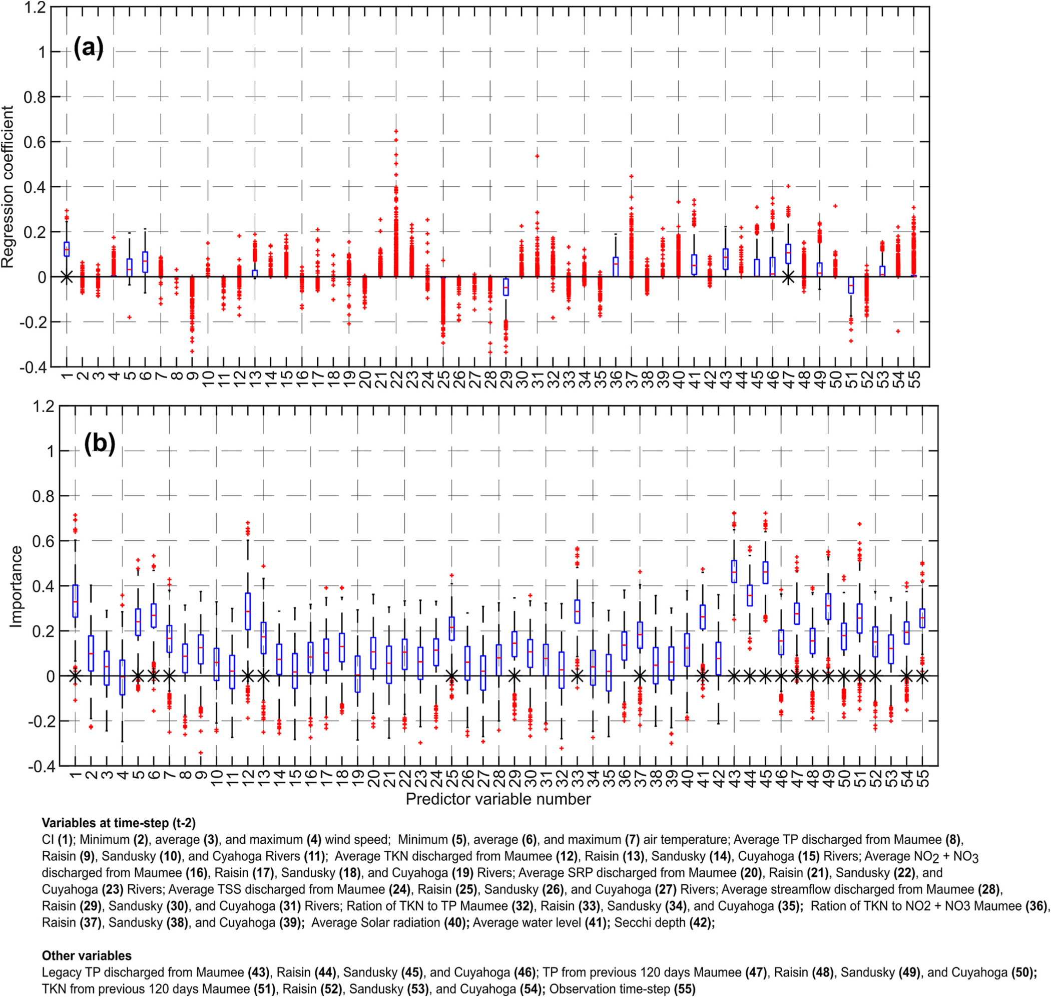
30-Day lead time forecast. Boxplots of the importance of the predictor variables obtained by using LASSO (top), and random forest (RF, bottom). These results were obtained using bootstrap sampling (BS) scheme. The symbol ‘*’ indicates that the variable was statistically significant at 5 % significance level.
3.3.1. CI
Both the algorithms recognized CI at the previous time step as an important predictor variable for the 10-, 20- and 30-day lead time forecasts. The importance of this predictor variable reduced as the lead time of the forecast increased. Since lag-1 CI is the most important of all the predictor variables, a LASSO model was trained and tested in the LOOCV scheme by using only the lag-1 CI as the predictor variable. The obtained by this strategy was equal to 0.49 compared to 0.55 when all the predictor variables were used. Thus, variables other than CI at the previous timestep do exert significant control over CyanoHAB growth.
3.3.2. Wind speed
The LASSO coefficients of the average and minimum wind speed at the previous time step were approximately zero for the 10-, 20- and 30-day lead time forecasts. The RF algorithm identified all three wind speed variables – minimum, average, and maximum wind speed – as unimportant. This seems reasonable since wind speed decreases CyanoHAB growth only if its magnitude is >5–7 m s−1 (Wynne et al., 2010), and within a 10-day period cyanobacteria would almost always get a few days with calm winds (Fig. S2 in SM), effectively reducing the importance of wind speed to forecast CyanoHAB cell count at the 10-day timescale.
Wind speed affects CyanoHAB growth because of the drag force it applies on the water surface. The drag force is directly proportional to the square of wind speed (Bengtsson, 1978). Therefore, one could argue that using the square of wind speed may make it an important predictor variable and improve the forecasting accuracy of the CI. We tested this hypothesis by training and testing a LASSO model in the LOOCV scheme and by using squares of the minimum, average, and maximum wind speeds as predictor variables, for 10-day lead time forecast. The obtained was 0.55, the same as obtained by using values of wind speed raised to power one as predictor variables. This result further asserts that wind speed at the previous time step is an unimportant predictor variable for CI forecast at the 10-day timescale. We also note that wind speed data used in this study may contain significant errors (Section S1 in SM) which might also result in reduced importance of this predictor variable.
3.3.3. Air temperature
In LASSO, the coefficients of minimum and average air temperature were typically positive for the 10-, 20- and 30-day lead time forecasts, as increased air temperature supports CyanoHAB growth. However, the values of these coefficients were only slightly greater than zero. The RF algorithm identified these two variables as unimportant for the 10-day lead time forecast but important for the 20- and 30-day lead time forecasts. Overall, results indicate that air temperature was a slightly important factor in explaining the variation in the CI values in Lake Erie, as was also concluded by Wynne et al. (2010). In most cases, the maximum air temperature was found to be an unimportant predictor variable according to both the LASSO and RF algorithms with the exception of 30-day lead time forecast by RF.
3.3.4. Nutrients, sediment loads, and streamflows during the previous 10 days
The results obtained by both the RF and LASSO suggest that the average TP, average TKN, and average streamflow at the previous time step were relatively unimportant predictors for the 10-day lead time forecast. It may be because nutrients discharged into the lake during the previous 10 days are not representative of the nutrients available for CyanoHAB growth in the lake. Another possibility is that the growth of CyanoHAB in the lake in limited by the nutrients discharged into the lake during the spring and early summer months, not by the nutrients discharged during the months of May-Oct. But some variables were identified as important by RF including TKN from the Sandusky and Cuyahoga Rivers, from the Sandusky River, TSS from the Raisin River, and the ratio of TKN to TP from the Raisin River.
Streamflow was an unimportant predictor variable based on both the RF and LASSO. The regression coefficients of streamflow were negative, consistent with the fact that higher streamflow implies a smaller residence time and a smaller growth rate. For the 30-day lead time forecast, streamflow from the Raisin River was an important predictor variable.
3.3.5. Solar radiation, water level, and Secchi depth
According to the RF, the importance of solar radiation increased as the lead time of forecast increased but remained statistically insignificant. For the 10-day lead time forecast, solar radiation at the time step did not play any role in determining the total CI according to the LASSO. For the 20- and 30-day lead time forecasts, the LASSO coefficients of solar radiation were almost always positive implying that higher solar radiation results in higher CyanoHAB growth. Average water level seems to be an important predictor variable according to the RF for all three lead-time forecasts; the regression coefficients of average water level were positive. Secchi depth was an unimportant predictor variable according to both the LASSO and RF algorithms.
3.3.6. Legacy nutrients
The TP discharged in the lake during the last 10 years (Legacy TP) from the Maumee, Raisin, and Sandusky Rivers were important predictor variables as suggested by the RF. The LASSO coefficients of these three variables were positive which indicates that higher legacy TP supports the growth of CyanoHAB. The importance of the legacy TP from the Cuyahoga River was lesser than those from the other three rivers. In this study, the legacy TP was used as a surrogate for the biologically available dissolved phosphate released to the water column from the lakebed. The results obtained affirm that phosphorous released from the lakebed is an important control over CyanoHAB growth (Ho and Michalak, 2017).
In addition to Legacy TP, TP discharged by all four rivers during the previous 120 days was an important predictor variable according to the RF and had positive regression coefficients for the 10-, 20- and 30-day lead time forecasts. This aligns with the evidence that increasing TP nutrient load in the lake during the spring months enhances CyanoHAB growth (Stumpf et al., 2012). TKN discharged in the lake during the previous 120 days from the Maumee, Raisin, and Cuyahoga Rivers were also important predictor variables. But the TKN discharged from the Sandusky River was not an important variable.
In summary, TP and TKN discharged into the lake during the previous 10 days were relatively unimportant. However, TP and TKN discharged into the lake during the previous 120 days were found to be important. This may be related to the mixing time of these nutrients into the lake and the time needed for particulate organic matter to be converted to biologically available nutrients for uptake and growth.
3.3.7. Observation time step
The RF algorithm showed that the observation time step was an important predictor variable for the 10-, 20-, and 30-day lead time forecasts. As noted earlier, providing the observation time step informs the model if the CyanoHAB dynamics is in the mortality or the growth phase.
3.4. Analysis with predictor variables at multiple time lags
Fig. 9 shows the values obtained by including the multiple-lag predictor variables in the BS scheme. Including the multiple lag variables slightly increased the value in most cases. For the 10-day lead time forecast, the highest of 0.61 was obtained by using the EA method. For the 20-day lead time forecast, the highest of 0.59 was obtained by using the RF model. For the 30-day lead time forecast, the highest of 0.53 was obtained by using the RF model.
Fig. 15 shows the observed and forecasted values of the logarithm of CI, in the LOOCV scheme, when the multiple-lag predictor variables were used along with the other predictor variables used in the previous section (as listed in Table 1). The inclusion of the multiple lag variables increased for the LASSO regression for the 10-day lead time forecast from 0.55 to 0.60. No improvements were obtained using the LASSO for 20- and 30-day lead time forecasts. Similarly, RF, ANN, and EA methods yielded null or only slight improvements. Therefore, this analysis alone does not tell us if the added multiple-lag predictor variables indeed better explain the variation in CI. To address this problem, the following analysis was conducted.
Fig. 15.
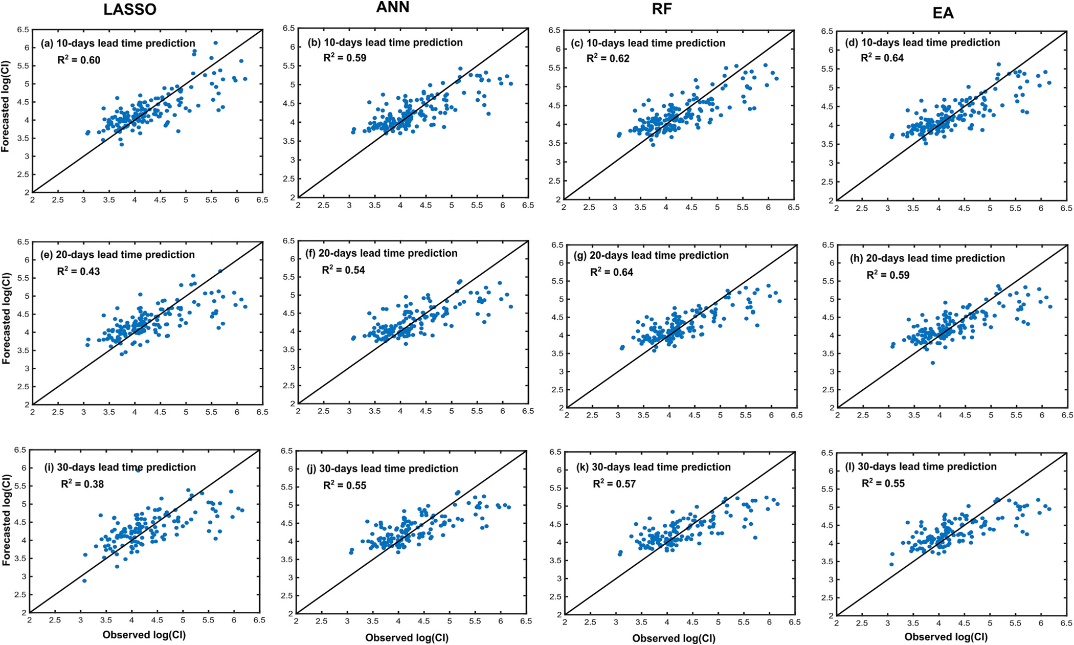
Observed and predicted logarithm of CI considering time-lagged predictor variables listed in Table 1 using LASSO (first column), ANN (second column), random forest (RF; third column), and average of ensemble (EA; fourth column). These results were obtained using leave-one-out cross-validation (LOOCV) scheme.
The predictor variables were ranked according to the median magnitude of their regression coefficients obtained by the LASSO in the BS scheme: the predictor variable with the highest value of the median of the regression coefficient was ranked 1, and so on. Then an RF regression analysis was carried out in the LOOCV scheme using an increasingly large number of predictor variables. For example, in the first iteration, only the predictor variable with rank 1 was used for the regression analysis. In the second iteration, only the predictor variables with ranks 1 and 2 were used for regression analysis, and so on. Thus, 72 (maximum number of predictors) regression analyses were carried out, and the mse and were computed for each of the analyses. The plotted mse and values obtained using these regression analyses are shown in Fig. 16. Note that this analysis was carried out for the 10-day lead time forecast.
Fig. 16.
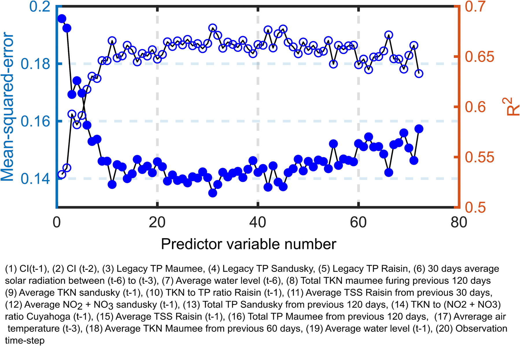
10-Day lead time prediction. Mean-square errors and coefficient of determination () computed by using the highest ranked predictor variables in RF regression. These results were obtained using leave-one-out-cross-validation (LOOCV) scheme using RF model.
The mse () decreased (increased) sharply by increasing the number of predictors from one highest-ranked to three highest-ranked. These three predictor variables in order of their rank were the CI at the time step , the CI at the time step , and the legacy TP from Maumee River. The mse further decreased until the 11 highest-ranked predictor variables were used for regression analysis – only small changes in mse values were seen beyond 11 predictor variables. Among these 11, the predictor variable with time-lag greater than one included the average solar radiation between the time steps and , the average water level at the time step , and the average TSS discharged from the Raisin river during the previous 30 days. Adding more predictor variables resulted in a further decrease (increase) in mse () values but at very slow rate, which reached the minimum (maximum) at 30. Other important multiple-lag predictors were the average air temperature at the time step , and the average TKN from the Maumee River during the previous 60 days. This analysis confirms that multiple-lag predictor variables indeed play a role in explaining the variation in CI.
The result that the 30-day average solar radiation during the time steps to are significantly more important than the average solar radiation during the time step to is puzzling and needs to be investigated in future studies. Also, the highest obtained by the RF regression was 0.68 when 30 highest-ranked predictor variables were used for regression analysis compared to when all the variables were used. This result indicates that the data are noisy, the sample size is small, and that there is a potential for more accurate forecasts if more data are used for training. This result also suggests that a careful selection of important predictor variables can result in more robust ML models compared to the models developed using all the predictor variables, when the sample size is small (e.g., Feng Chang et al., 2023).
4. Summary and conclusions
The lack of in-situ data is a major hurdle in modeling the CyanoHAB dynamic in Lake Erie. Also, the coupled hydrodynamic and CyanoHAB growth dynamic models are costly to run and require significant computational effort. In this study, four data-driven models LASSO, RF, ANN, and an ensemble average of these three models (EA) along with remote sensing data were used to forecast CyanoHAB cell count at 10-, 20-, and 30-day lead time. Also, the important variables for forecasting were identified. Remote sensing data were used to derive a surrogate for CyanoHAB cell count, referred to as cyanobacterial index (CI). Overall, the results were encouraging, and it appears that the CyanoHAB cell counts in Lake Erie are predictable at 10-, 20- and 30-day lead time. Among the four data-driven models used in this study, RF and EA performed better than LASSO and ANN. The poorer performance of LASSO is not surprising since it can only capture linear relationships between predictor and response variables. The difference between the performance of the RF and the LASSO algorithms was significant for 20- and 30-day lead time forecasts. The reason for the poorer performance of the ANN algorithm compared to RF is unclear and a more definitive comparison would need a larger sample size. The performance of RF and EA were similar. The highest obtained for 10-day lead time forecast was 0.68 when thirty most important predictor variables were used.
Residual analysis revealed that a symmetric and heavy-tailed distribution was a suitable choice for modeling the residuals. The predictive uncertainty bounds obtained by the residual analysis were very wide. We note that part of this uncertainty comes from uncertainty in CI observations since the CI values used were based on remote sensing data. Further, the relationship between CI and CyanoHAB cell count has some scatter which contributes to predictive uncertainty. Therefore, it appears that advances in remote sensing technology will increase the model performance and reduce the predictive uncertainty.
The best predictor of CyanoHAB cell count for 10-, 20-, and 30-day lead time forecasts is the cell count at the current time step, thus, indicating temporal memory at 10-, 20-, and 30-day timescale. Among other predictor variables, time-integrated variables such as legacy TP (TP discharged over the previous 10 years) and TP discharged during the previous 120 days were important. The importance of predictor variables such as average TP, TKN, and streamflow at 10-day lag period was inconclusive. Similarly, variables such as wind speed, and Secchi depth over 10-day lag period were not important but water level averaged over a 10-day lag period was an important variable. Water levels were positively correlated with CI. The air temperature was only a slightly important variable. It appears that CyanoHAB intensity at sub-monthly timescales is mainly determined by the coarser timescale variables and biological processes of CyanoHABs. Surprisingly, the 30-day average solar radiation between the time steps and , and water level at the time step were important variables in determining CyanoHAB dynamics.
CI values themselves are a proxy for CyanoHAB cell count. In this study, the relationships of CI with in-situ measured phycocyanin concentration (volume and areal), chlorophyll-a concentration, and Microcystis biovolume were established. The first two relationships were good. But a significant scatter around the 1:1 line was observed. This scatter was partly due to a mismatch between the spatial scales of in-situ measurements and satellite-derived CI measurements. More in-situ data are required to reduce the uncertainty in these relationships.
One of the limitations of the study was that data from the Detroit River was not used in developing the models because of extreme sparsity of water quality data available from this river. It is the largest river (by volume) flowing into Lake Erie with a significant impact on the residence time of lake water. As was noted earlier, the largest source of nutrients in the lake is the Maumee River (Sayers et al., 2016; Muenich et al., 2016). Nevertheless, data from the Detroit River may result in better performing models. The effect of missing information regarding nutrients inputs to the lake on HAB modeling is a topic for future studies. Another limitation of this study was the small number of samples used for the analysis along with the uncertainties associated with several of the measured variables. For example, air temperature and wind speed data are likely to be highly uncertain. Generating a large sample size would not be possible for Lake Erie in the near future as a maximum of 19 samples can be collected for each year (one for each 10-day time window). An alternative is to use data across several different lakes to pool the information. Future work may also accommodate various uncertainties associated with different data and models in a Bayesian framework that would allow us to gain better insights into CyanoHAB growth dynamics in Lake Erie. The challenge is that such a framework would require an understanding of the statistical structure of errors, and such information is not readily available and would have to be inferred, if at all possible, from the limited data.
Supplementary Material
Fig. 13.
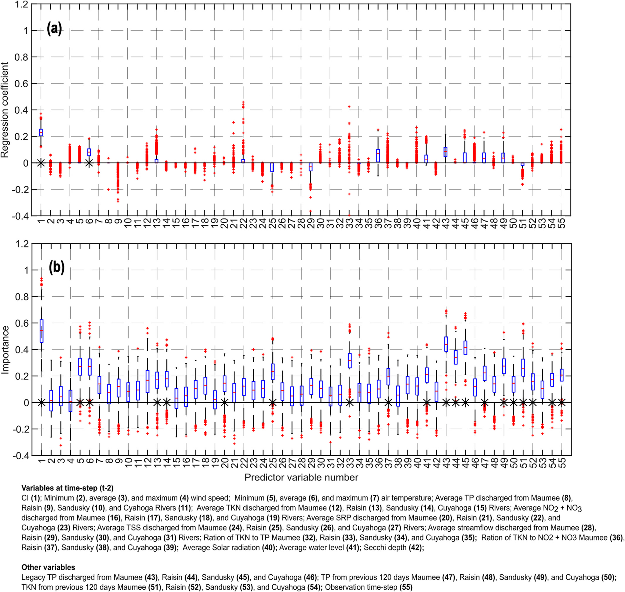
20-Day lead time forecast. Boxplots of the importance of the predictor variables obtained by using LASSO (top), and random forest (RF, bottom). These results were obtained using bootstrap sampling (BS) scheme. The symbol ‘*’ indicates that the variable was statistically significant at 5 % significance level.
Acknowledgement
The U.S. Environmental Protection Agency through its Office of Research and Development funded and managed the research described here under EPA Contract #EP-C-15-010. This document has been reviewed in accordance with U.S. Environmental Protection Agency policy and approved for publication. The views expressed in this article are those of the author(s) and do not necessarily represent the views or policies of the U.S. Environmental Protection Agency. AG was partially funded by DRI’s postdoctoral support funds during the preparation of this manuscript. We thank an anonymous reviewer for useful comments on an earlier draft of the paper that helped us improve the paper substantially.
Footnotes
Declaration of competing interest
The authors declare the following financial interests/personal relationships which may be considered as potential competing interests: Abhinav Gupta reports financial support was provided by United States Environmental Protection Agency.
CRediT authorship contribution statement
Abhinav Gupta: Conceptualization, Methodology, Formal analysis, Data curation, Writing – original draft, Visualization. Mohamed M. Hantush: Conceptualization, Funding acquisition, Writing – review & editing. Rao S. Govindaraju: Conceptualization, Funding acquisition, Writing – review & editing, Supervision.
Appendix A. Supplementary data
Supplementary data to this article can be found online at https://doi.org/10.1016/j.scitotenv.2023.165781.
Data relevant to this paper can be found at manuscript data.
Data availability
The link to data have been provided in the manuscript.
References
- Abu-Mostafa YS, Magdon-Ismail M, Lin HT, 2012. Learning from data, vol. 4. AMLBook, New York, NY, USA. [Google Scholar]
- Baker DB, Confesor R, Ewing DE, Johnson LT, Kramer JW, Merryfield BJ, 2014. Phosphorus loading to Lake Erie from the Maumee, Sandusky and Cuyahoga rivers: the importance of bioavailability. J. Great Lakes Res. 40 (3), 502–517. [Google Scholar]
- Beletsky D, Hawley N, Rao YR, 2013. Modeling summer circulation and thermal structure of Lake Erie. J. Geophys. Res. Oceans 118 (11), 6238–6252. [Google Scholar]
- Bengtsson L, 1978. Wind induced circulation in lakes. Hydrol. Res. 9 (2), 75–94. [Google Scholar]
- Box GE, Tiao GC, 1973. Bayesian Inference in Statistical Analysis. John Wiley & Sons. [Google Scholar]
- Breiman L, 2001. Random forests. Mach. Learn. 45 (1), 5–32. [Google Scholar]
- Bridgeman TB, Chaffin JD, Filbrun JE, 2013. A novel method for tracking western Lake Erie Microcystis blooms, 2002–2011. J. Great Lakes Res. 39 (1), 83–89. [Google Scholar]
- Burtner A, Palladino D, Kitchens C, Fyffe D, Johengen T, Stuart D, Cooperative Institute for Great Lakes Research, University of Michigan, Fanslow, David, Gossiaux, Duane, National Oceanic and Atmospheric Administration, Great Lakes Environmental Research Laboratory, 2019. Physical, Chemical, and Biological Water Quality Data Collected From a Small Boat in Western Lake Erie, Great Lakes From 2012-05-15 to 2018-10-09 (NCEI Accession 0187718). [Indicate Subset Used]. NOAA National Centers for Environmental Information. Dataset. https://accession.nodc.noaa.gov/0187718. (Accessed January 2020). [Google Scholar]
- Chaffin JD, Bridgeman TB, Heckathorn SA, Mishra S, 2011. Assessment of Microcystis growth rate potential and nutrient status across a trophic gradient in western Lake Erie. J. Great Lakes Res. 37 (1), 92–100. [Google Scholar]
- Chaffin JD, Bridgeman TB, Bade DL, 2013. Nitrogen constrains the growth of late summer cyanobacterial blooms in Lake Erie. Adv. Microbiol. 2013. [Google Scholar]
- Cheng RT, Powell TM, Dillon TM, 1976. Numerical models of wind-driven circulation in lakes. Appl. Math. Model. 1 (3), 141–159. [Google Scholar]
- Den Uyl PA, Harrison SB, Godwin CM, Rowe MD, Strickler JR, Vanderploeg HA, 2021. Comparative analysis of Microcystis buoyancy in western Lake Erie and Saginaw Bay of Lake Huron. Harmful Algae 108, 102102. [DOI] [PubMed] [Google Scholar]
- Deng T, Chau KW, Duan HF, 2021. Machine learning based marine water quality prediction for coastal hydro-environment management. J. Environ. Manag. 284, 112051. [DOI] [PubMed] [Google Scholar]
- European Space Agency, 2006. MERIS Product Handbook Issue 2.1, 24th October. [Google Scholar]
- Fahnenstiel GL, Millie DF, Dyble J, Litaker RW, Tester PA, McCormick MJ, Klarer D, 2008. Microcystin concentrations and cell quotas in Saginaw Bay, Lake Huron. Aquat. Ecosyst. Health Manag. 11 (2), 190–195. [Google Scholar]
- Fastner J, Abella S, Litt A, Morabito G, Vörös L, Pálffy K, Chorus I, 2016. Combating cyanobacterial proliferation by avoiding or treating inflows with high P load—experiences from eight case studies. Aquat. Ecol. 50 (3), 367–383. [Google Scholar]
- Feng Chang C, Astitha M, Yuan Y, Tang C, Vlahos P, Garcia V, Khaira U, 2023. A new approach to predict tributary phosphorus loads using machine learning and physics-based modeling systems. Artif. Intel. Earth Syst. 1–43. [DOI] [PMC free article] [PubMed] [Google Scholar]
- Fernández C, Steel MF, 1998. On Bayesian modeling of fat tails and skewness. J. Am. Stat. Assoc. 93 (441), 359–371. [Google Scholar]
- Franks PJ, 2018. Recent advances in modelling of harmful algal blooms. Glob. Ecol. Oceanogr. Harmful Algal Blooms 359–377. [Google Scholar]
- Friedman J, Hastie T, Tibshirani R, 2001. The Elements of Statistical Learning, vol. 1, No. 10. Springer, New York (series in statistics.). [Google Scholar]
- Handler AM, Compton JE, Hill RA, Leibowitz SG, Schaeffer BA, 2023. Identifying lakes at risk of toxic cyanobacterial blooms using satellite imagery and field surveys across the United States. Sci. Total Environ. 869, 161784. [DOI] [PMC free article] [PubMed] [Google Scholar]
- Haykin S, 2009. Neural Networks and Learning Machines, 3/E. Pearson Education India. [Google Scholar]
- Ho JC, Michalak AM, 2017. Phytoplankton blooms in Lake Erie impacted by both long-term and springtime phosphorus loading. J. Great Lakes Res. 43 (3), 221–228. [Google Scholar]
- Ho JC, Michalak AM, Pahlevan N, 2019. Widespread global increase in intense lake phytoplankton blooms since the 1980s. Nature 574 (7780), 667–670. [DOI] [PubMed] [Google Scholar]
- Huisman J, Hulot FD, 2005. Population dynamics of harmful cyanobacteria. Factors affecting species composition. In: Harmful cyanobacteria, pp. 143–176. [Google Scholar]
- Huisman J, Codd GA, Paerl HW, Ibelings BW, Verspagen JM, Visser PM, 2018. Cyanobacterial blooms. Nat. Rev. Microbiol. 16 (8), 471–483. [DOI] [PubMed] [Google Scholar]
- Huntington JL, Hegewisch KC, Daudert B, Morton CG, Abatzoglou JT, McEvoy DJ, Erickson T, 2017. Climate engine: cloud computing and visualization of climate and remote sensing data for advanced natural resource monitoring and process understanding. Bull. Am. Meteorol. Soc. 98 (11), 2397–2410. [Google Scholar]
- Kotut K, Ballot A, Krienitz L, 2006. Toxic cyanobacteria and their toxins in standing waters of Kenya: implications for water resource use. J. Water Health 4 (2), 233–245. [PubMed] [Google Scholar]
- Kromkamp J, Konopka A, Mur LR, 1988. Buoyancy regulation in light-limited continuous cultures of Microcystis aeruginosa. J. Plankton Res. 10 (2), 171–183. [Google Scholar]
- Kutser T, 2004. Quantitative detection of chlorophyll in cyanobacterial blooms by satellite remote sensing. Limnol. Oceanogr. 49 (6), 2179–2189. [Google Scholar]
- Leon LF, Smith RE, Hipsey MR, Bocaniov SA, Higgins SN, Hecky RE, Guildford SJ, 2011. Application of a 3D hydrodynamic–biological model for seasonal and spatial dynamics of water quality and phytoplankton in Lake Erie. J. Great Lakes Res. 37 (1), 41–53. [Google Scholar]
- Liu G, Simis SG, Li L, Wang Q, Li Y, Song K, Shi K, 2017. A four-band semi-analytical model for estimating phycocyanin in inland waters from simulated MERIS and OLCI data. IEEE Trans. Geosci. Remote Sens. 56 (3), 1374–1385. [Google Scholar]
- Ma R, Kong W, Duan H, Zhang S, 2009. Quantitative estimation of phycocyanin concentration using MODIS imagery during the period of cyanobacterial blooming in Taihu Lake. China Environ. Sci. 29 (3), 254–260. [Google Scholar]
- Michalak AM, Anderson EJ, Beletsky D, Boland S, Bosch NS, Bridgeman TB, DePinto JV, 2013. Record-setting algal bloom in Lake Erie caused by agricultural and meteorological trends consistent with expected future conditions. Proc. Natl. Acad. Sci. 110 (16), 6448–6452. [DOI] [PMC free article] [PubMed] [Google Scholar]
- Millie DF, Weckman GR, Fahnenstiel GL, Carrick HJ, Ardjmand E, Young WA, Shuchman RA, 2014. Using artificial intelligence for CyanoHAB niche modeling: discovery and visualization of Microcystis–environmental associations within western Lake Erie. Can. J. Fish. Aquat. Sci. 71 (11), 1642–1654. [Google Scholar]
- Mishra S, Stumpf RP, Schaeffer BA, Werdell PJ, Loftin KA, Meredith A, 2019. Measurement of cyanobacterial bloom magnitude using satellite remote sensing. Sci. Rep. 9 (1), 18310. [DOI] [PMC free article] [PubMed] [Google Scholar]
- Mitrovic SM, Hardwick L, Dorani F, 2011. Use of flow management to mitigate cyanobacterial blooms in the Lower Darling River, Australia. J. Plankton Res. 33 (2), 229–241. [Google Scholar]
- Muenich RL, Kalcic M, Scavia D, 2016. Evaluating the impact of legacy P and agricultural conservation practices on nutrient loads from the Maumee River Watershed. Environ. Sci. Technol. 50 (15), 8146–8154. [DOI] [PubMed] [Google Scholar]
- NCWQR, 2022. Heidelberg Tributary Loading Program (HTLP) Dataset. Zenodo. 10.5281/zenodo.6606949. [DOI] [Google Scholar]
- Paerl HW, Huisman J, 2009. Climate change: a catalyst for global expansion of harmful cyanobacterial blooms. Environ. Microbiol. Rep. 1 (1), 27–37. [DOI] [PubMed] [Google Scholar]
- Paerl HW, Otten TG, 2013. Harmful cyanobacterial blooms: causes, consequences, and controls. Microb. Ecol. 65 (4), 995–1010. [DOI] [PubMed] [Google Scholar]
- Ranjbar MH, Hamilton DP, Etemad-Shahidi A, Helfer F, 2021. Individual-based modelling of cyanobacteria blooms: physical and physiological processes. Sci. Total Environ. 792, 148418. [DOI] [PubMed] [Google Scholar]
- Reinart A, Kutser T, 2006. Comparison of different satellite sensors in detecting cyanobacterial bloom events in the Baltic Sea. Remote Sens. Environ. 102 (1–2), 74–85. [Google Scholar]
- Reitz LA, 2020. Quantification of Microcystin Production and Loss Rates for the Spatiotemporal Distribution of Microcystis aeruginosa Blooms in Lake Erie (Doctoral dissertation,. Bowling Green State University. [Google Scholar]
- Reutter JM, 2019. Lake Erie: past, present, and future. In: Encyclopedia of Water: Science, Technology, and Society, pp. 1–15. [Google Scholar]
- Rinta-Kanto JM, Konopko EA, DeBruyn JM, Bourbonniere RA, Boyer GL, Wilhelm SW, 2009. Lake Erie Microcystis: relationship between microcystin production, dynamics of genotypes and environmental parameters in a large lake. Harmful Algae 8 (5), 665–673. [Google Scholar]
- Rousso BZ, Bertone E, Stewart R, Hamilton DP, 2020. A systematic literature review of forecasting and predictive models for cyanobacteria blooms in freshwater lakes. Water Res. 182, 115959. [DOI] [PubMed] [Google Scholar]
- Sayers M, Fahnenstiel GL, Shuchman RA, Whitley M, 2016. Cyanobacteria blooms in three eutrophic basins of the Great Lakes: a comparative analysis using satellite remote sensing. Int. J. Remote Sens. 37 (17), 4148–4171. [Google Scholar]
- Scheffer M, Rinaldi S, Huisman J, Weissing FJ, 2003. Why plankton communities have no equilibrium: solutions to the paradox. Hydrobiologia 491 (1–3), 9–18. [Google Scholar]
- Soontiens N, Binding C, Fortin V, Mackay M, Rao YR, 2019. Algal bloom transport in Lake Erie using remote sensing and hydrodynamic modelling: sensitivity to buoyancy velocity and initial vertical distribution. J. Great Lakes Res. 45 (3), 556–572. [Google Scholar]
- Stow CA, Cha Y, Johnson LT, Confesor R, Richards RP, 2015. Long-term and seasonal trend decomposition of Maumee River nutrient inputs to western Lake Erie. Environ. Sci. Technol. 49 (6), 3392–3400. [DOI] [PubMed] [Google Scholar]
- Stumpf RP, Wynne TT, Baker DB, Fahnenstiel GL, 2012. Interannual variability of cyanobacterial blooms in Lake Erie. PLoS One 7 (8), e42444. [DOI] [PMC free article] [PubMed] [Google Scholar]
- Stumpf RP, Johnson LT, Wynne TT, Baker DB, 2016. Forecasting annual cyanobacterial bloom biomass to inform management decisions in Lake Erie. J. Great Lakes Res. 42 (6), 1174–1183. [Google Scholar]
- Verhamme EM, Redder TM, Schlea DA, Grush J, Bratton JF, DePinto JV, 2016. Development of the Western Lake Erie Ecosystem Model (WLEEM): application to connect phosphorus loads to cyanobacteria biomass. J. Great Lakes Res. 42 (6), 1193–1205. [Google Scholar]
- Visser PM, Ibelings BW, Bormans M, Huisman J, 2016. Artificial mixing to control cyanobacterial blooms: a review. Aquat. Ecol. 50 (3), 423–441. [Google Scholar]
- Wallace BB, Bailey MC, Hamilton DP, 2000. Simulation of vertical position of buoyancy regulating Microcystis aeruginosa in a shallow eutrophic lake. Aquat. Sci. 62 (4), 320–333. [Google Scholar]
- Welander P, 1957. Wind action on a shallow sea: some generalizations of Ekman’s theory. Tellus 9 (1), 45–52. [Google Scholar]
- Wilhelm SW, Bullerjahn GS, McKay RML, 2020. The complicated and confusing ecology of Microcystis blooms. Mbio 11 (3) (e00529–20). [DOI] [PMC free article] [PubMed] [Google Scholar]
- Wynne TT, Stumpf RP, 2015. Spatial and temporal patterns in the seasonal distribution of toxic cyanobacteria in western Lake Erie from 2002–2014. Toxins 7 (5), 1649–1663. [DOI] [PMC free article] [PubMed] [Google Scholar]
- Wynne TT, Stumpf RP, Tomlinson MC, Dyble J, 2010. Characterizing a cyanobacterial bloom in western Lake Erie using satellite imagery and meteorological data. Limnol. Oceanogr. 55 (5), 2025–2036. [Google Scholar]
- Yan Y, Bao Z, Shao J, 2018. Phycocyanin concentration retrieval in inland waters: a comparative review of the remote sensing techniques and algorithms. J. Great Lakes Res. 44 (4), 748–755. [Google Scholar]
- You J, Mallery K, Hong J, Hondzo M, 2018. Temperature effects on growth and buoyancy of Microcystis aeruginosa. J. Plankton Res. 40 (1), 16–28. [Google Scholar]
- Zhu Y, Feng Y, Browning TJ, Wen Z, Hughes DJ, Hao Q, Chai F, 2022. Exploring variability of trichodesmium photophysiology using multi-excitation wavelength fast repetition rate fluorometry. Front. Microbiol. 13. [DOI] [PMC free article] [PubMed] [Google Scholar]
- Zolfaghari K, Duguay CR, 2016. Estimation of water quality parameters in lake Erie from MERIS using linear mixed effect models. Remote Sens. 8 (6), 473. [Google Scholar]
Associated Data
This section collects any data citations, data availability statements, or supplementary materials included in this article.
Supplementary Materials
Data Availability Statement
The link to data have been provided in the manuscript.


