Software Application Profile: The daggle app—a tool to support learning and teaching the graphical rules of selecting adjustment variables using directed acyclic graphs

Abstract

Motivation

Directed acyclic graphs (DAGs) are used in epidemiological research to communicate causal assumptions and guide the selection of covariate adjustment sets when estimating causal effects. For any given DAG, a set of graphical rules can be applied to identify minimally sufficient adjustment sets that can be used to adjust for bias due to confounding when estimating the causal effect of an exposure on an outcome. The daggle app is a web-based application that aims to assist in the learning and teaching of adjustment set identification using DAGs.

General features

The application offers two modes: tutorial and random. The tutorial mode presents a guided introduction to how common causal structures can be presented using DAGs and how graphical rules can be used to identify minimally sufficient adjustment sets for causal estimation. The random mode tests this understanding by presenting the user with a randomly generated DAG—a daggle. To solve the daggle, users must correctly identify a valid minimally sufficient adjustment set.

Implementation

The daggle app is implemented as an R shiny application using the golem framework. The application builds upon existing R libraries including pcalg to generate reproducible random DAGs, dagitty to identify all valid minimal adjustment sets and ggdag to visualize DAGs.

Availability

The daggle app can be accessed online at [http://cbdrh.shinyapps.io/daggle]. The source code is available on GitHub [https://github.com/CBDRH/daggle] and is released under a Creative Commons CC BY-NC-SA 4.0 licence.

Introduction

Directed acyclic graphs (DAGs) allow researchers to formalize and communicate their assumptions regarding the data generation mechanism(s) underlying causal research questions and to identify appropriate covariate adjustment sets to minimize bias when estimating causal effects of interest. A growing body of theoretical expositions^1,2 and applied tutorials^3–7 demonstrates how DAGs can be used to support causal inference. Here we describe the daggle app, a gamified, web-based application that aims to support teaching and learning the graphical rules for covariate selection from a DAG.

The task of identifying appropriate covariate adjustment sets from a given DAG can be automated using computationally efficient implementation of graphical rules. Software solutions are convenient and essential for more complex DAGs where manually applying graphical rules quickly becomes intractable. Whereas several software options are available to support identification of minimally sufficient adjustment sets,^9–13 it is critical for researchers to have a thorough understanding of the concepts and rules underlying DAGs to support appropriate application in their research.¹⁴

The daggle app aims to help foster this understanding by using a gamified approach to learning the underlying graphical rules of causal DAG theory. Whereas existing applications present users with a valid adjustment set for a given DAG, the daggle app has an educational focus and requires the user to reason out the solution. Users are presented with a randomly generated causal DAG—a daggle—and must provide a solution by correctly identifying a minimally sufficient covariate adjustment set. Recent research has shown that gamified approaches to statistical education can improve students’ experience and performance.^15,16 By choosing a gamified rather than didactic exposition, we aim to make the learning experience accessible and playful, and to help researchers—from students to senior faculty—build an intuitive understanding of the graphical rules for adjustment variable selection from DAGs. We hope that a thorough understanding of these foundational rules will help to build students’ and practitioners’ confidence in applying DAG-based covariate selection.

Understanding the graphical rules for covariate selection from a DAG

To use the daggle app, users must apply a set of graphical rules to identify a minimally sufficient adjustment set, i.e. the smallest subset of covariates that is sufficient to obtain an unbiased estimate of the causal effect of interest. Here we briefly review those rules.

Figure 1 shows a causal DAG with an exposure $\mathrm{X}$, outcome $\mathrm{Y}$ and three additional variables ${\mathrm{Z}}_1$, ${\mathrm{Z}}_2$ and ${\mathrm{Z}}_3$. A directed or causal path on a DAG is a path where all the arrows along the path point from the exposure to the outcome. For example, in Figure 1, the path $\mathrm{X}\to \mathrm{Y}$ is a causal path. The path $\mathrm{X}\to {\mathrm{Z}}_2\to \mathrm{Y}$ is also a causal path. Here, ${\mathrm{Z}}_2$ is a mediator, or a variable along the causal path from X to Y (i.e. ${\mathrm{Z}}_2$ is caused by X and causes Y). A non-causal path is a path from the exposure to outcome where one or more arrows along the path point back towards the exposure. In Figure 1, the path $\mathrm{X}\leftarrow {\mathrm{Z}}_1\to \mathrm{Y}$ is a backdoor path, an example of a non-causal path which starts with an arrow pointing towards the exposure $\mathrm{X}$. Importantly, the absence of arrow between two nodes in a DAG carries the strongest assumptions. For example, this DAG assumes that $\mathrm{X}$ has no effect on ${\mathrm{Z}}_3$.

Figure 1.

An example directed acyclic graph (DAG)

Paths on a DAG are open if they transmit statistical association, otherwise they are closed. In Figure 1, the path $\mathrm{X}\leftarrow {\mathrm{Z}}_1\to \mathrm{Y}$ is an open backdoor or confounding path. On this path, ${\mathrm{Z}}_1$ is a confounder of the effect of the exposure on the outcome, so even in the absence of a direct causal effect of $\mathrm{X}$ on $\mathrm{Y},$ we would expect to find a statistical association between $\mathrm{X}$ and $\mathrm{Y}$ in the presence of confounding. There is a second non-causal path in Figure 1, the path $\mathrm{X}\to {\mathrm{Z}}_2\leftarrow {\mathrm{Z}}_3\to \mathrm{Y}$. This path is closed at ${\mathrm{Z}}_2$ because there is no implied statistical association between $\mathrm{X}$ and $\mathrm{Y}$, which we explain in further detail below.

To estimate the total effect of an exposure on an outcome, all open non-causal paths between the exposure and outcome must be closed, a condition referred to as the backdoor criterion.¹ To estimate the direct effect of an exposure on an outcome, excluding any mediated effects, it is also necessary to close any causal paths apart from the direct path of interest $\mathrm{X}\to \mathrm{Y}$.

A simple way to graphically confirm whether a path is open or closed is to examine each consecutive triplet of nodes along the path: if any triplet is closed, the entire path is closed. Given any three consecutive nodes on a path, three possible combinations arise (Figure 2). The path ${\mathrm{Z}}_1\to {\mathrm{Z}}_2\to {\mathrm{Z}}_3$ is open, and controlling for ${\mathrm{Z}}_2$ will close the path. Similarly, the path ${\mathrm{Z}}_1\leftarrow {\mathrm{Z}}_2\to {\mathrm{Z}}_3$ is open, and controlling for ${\mathrm{Z}}_2$ will close the path. In contrast, the path ${\mathrm{Z}}_1\to {\mathrm{Z}}_2\leftarrow {\mathrm{Z}}_3$ is closed. Here, controlling for ${\mathrm{Z}}_2$ will open the path. In this final example, ${\mathrm{Z}}_2$ is a collider because the arrows from ${\mathrm{Z}}_1$ and ${\mathrm{Z}}_3$ collide at ${\mathrm{Z}}_2$. Paths on a DAG are closed at uncontrolled colliders, and no statistical association is transmitted along these paths. Controlling for a collider can potentially open a non-causal path between the exposure and outcome, resulting in collider stratification bias.

Figure 2.

Examples of open and closed paths, and the effect of conditioning in three different scenarios

Returning to Figure 1, to estimate the total effect of $\mathrm{X}$ on $\mathrm{Y}$, it would be necessary to close the open backdoor path $\mathrm{X}\leftarrow {\mathrm{Z}}_1\to \mathrm{Y}$. The path can be closed by adjusting for ${\mathrm{Z}}_1$ in the analysis, for example by including ${\mathrm{Z}}_1$ as a covariate in a regression of $\mathrm{Y}$ on $\mathrm{X}$. To estimate the direct effect of $\mathrm{X}$ on $\mathrm{Y}$, excluding any mediated effects, it would be necessary to control for ${\mathrm{Z}}_1$ to close the open backdoor path $\mathrm{X}\leftarrow {\mathrm{Z}}_1\to \mathrm{Y}$, and also to control for the mediator ${\mathrm{Z}}_2$ to close the open causal path $\mathrm{X}\to {\mathrm{Z}}_2\to \mathrm{Y}$. However, in this example, controlling for ${\mathrm{Z}}_2$ has the effect of opening the non-causal path $\mathrm{X}\to {\mathrm{Z}}_2\leftarrow {\mathrm{Z}}_3\to \mathrm{Y}$. This is because although ${\mathrm{Z}}_2$ is a mediator on the path $\mathrm{X}\to {\mathrm{Z}}_2\to \mathrm{Y}$, it is also a collider on the path $\mathrm{X}\to {\mathrm{Z}}_2\leftarrow {\mathrm{Z}}_3\to \mathrm{Y}$ (i.e. the arrows from $\mathrm{X}$ and ${\mathrm{Z}}_3$ collide at ${\mathrm{Z}}_2$) and controlling for a collider opens a path. This newly opened path can be closed by controlling for ${\mathrm{Z}}_3$, an example of a mediator-outcome confounder. So, to estimate the direct effect of $\mathrm{X}$ on $\mathrm{Y}$ in this example, it is necessary to control for ${\mathrm{Z}}_1$, ${\mathrm{Z}}_2$ and ${\mathrm{Z}}_3$.

To review, using a DAG to identify a minimally sufficient adjustment set to identify the total effect of an exposure $\mathrm{X}$ on an outcome $\mathrm{Y}$ amounts to identifying all open non-causal paths between $\mathrm{X}$ and $\mathrm{Y}$ and selecting the smallest set of adjustment variables necessary to close these paths. To identify the direct effect of $\mathrm{X}$ on $\mathrm{Y}$ it is also necessary to close any mediated causal paths, while taking care not to control for a mediator which is also a collider on a separate path. Doing so can open new non-causal paths which will also need to be closed to avoid collider stratification bias.³

Implementation

daggle is a web-based app implemented using the shiny web application framework for R¹⁷ and developed following the golem schema for shiny apps.¹⁸ The app builds on several functions implemented in R, including the randomDAG() function from the pcalg package¹³ to generate a pseudo-random DAG, the adjustmentSets() function from the dagitty package¹⁰ to identify the minimally sufficient adjustment sets for the generated DAG, and ggdag functions to visualize the generated DAG and corresponding solutions. The app is deployed online to a shinyapps.io server and can be accessed using a desktop or mobile browser. Source code for the daggle app is available on GitHub [https://github.com/CBDRH/daggle] and is released under a Creative Commons CC BY-NC-SA 4.0 licence.

Use

The daggle app offers two modes: tutorial and random. The tutorial mode presents a guided introduction describing how common causal structures of confounding, mediation and collider bias can be represented using DAGs and how graphical rules can be used to identify minimally sufficient adjustment sets to estimate the causal effect of an exposure on an outcome. Users are presented with a series of vignettes and must select adjustment variables to identify either total or direct effects.

The random mode presents the user with a randomly generated causal DAG—a daggle (Figure 3). To solve the daggle, users must identify a minimally sufficient adjustment set to obtain an unbiased estimate of the specified effect and click or tap on the corresponding variables to indicate their selection. Clicking or tapping on a variable changes the shape and colour of the node, with grey circles indicating unadjusted variables and pink squares indicating adjusted variables. In some cases, the specified effect can be estimated without any adjustment, in which case the user leaves all variables unadjusted.

Figure 3.

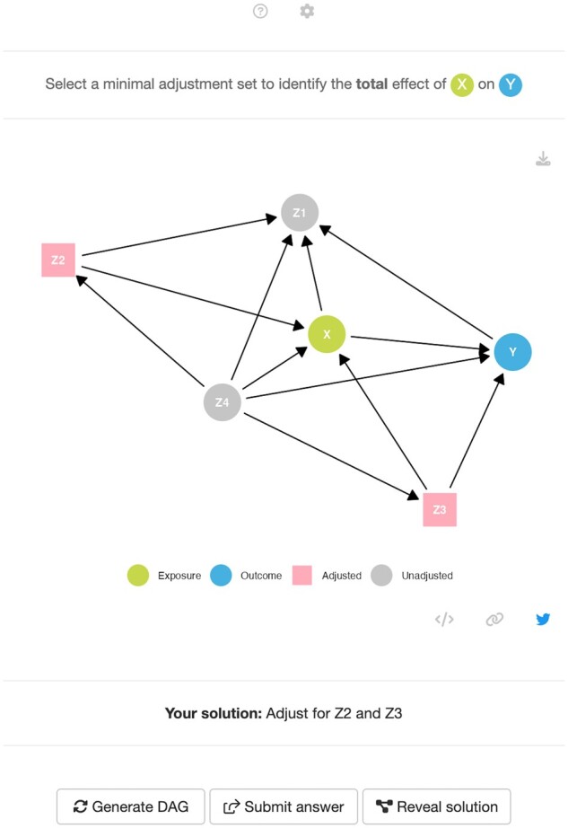
A screenshot of the daggle app in random mode, with variables Z₂ and Z₃ selected for adjustment. Try to solve this daggle at [cbdrh.shinyapps.io/daggle/?_values_&id=145590]

When playing in random mode, users can specify the number of nodes (from three to eight) and the complexity of the DAG (easy, moderate or hard). The DAG complexity determines the probability of connecting a node to another node in the random DAG generation algorithm, with the easy, moderate and hard settings corresponding to probabilities 40%, 60% and 80%, respectively. Users can also choose between the total or direct effect as the causal effect of interest. To correctly identify the total effect of the exposure on the outcome, all non-causal paths must be closed. To identify the direct effect, all non-causal paths must be closed as well as any causal path apart from the direct path $\mathrm{X}\to \mathrm{Y}$.

Once a user has selected their answer, they can tap or click on the Submit Answer button. If correct, they are given randomly generated praise (e.g. ‘Correct! Absolutely fabulous!’) and prompted to generate a new daggle. If they submit a valid adjustment set which is not a minimally sufficient adjustment set, a message will appear to indicate this. If their submission is incorrect, they are given randomly generated encouragement (e.g. ‘Try it again. I have a good feeling about this.’) and prompted to enter another solution or to launch a hint. The hint screen restates the desired estimand and displays the open and closed causal and non-causal paths based on their current submission. At any time, the user can click or tap on the Reveal Solution button to see all the valid minimally sufficient adjustment sets for the given daggle.

The app provides three ways to reproduce or share the randomly generated DAGs and the tutorial DAGs. Clicking on the download icon will download a local .png version of the DAG. Clicking on the code icon provides the model code to reproduce the DAG on dagitty.net or in the R implementation of dagitty. Clicking on the link icon will generate a unique URL, allowing the user to share or return to a specific daggle.

Discussion

Using DAGs to inform modelling decisions is increasingly popular in epidemiological research. The daggle app aims to support epidemiologists to teach and learn the basic graphical rules for using DAGs to identify minimally sufficient adjustment sets. Combining randomly generated DAGs with algorithmically derived solutions in a simple interface avoids the need for an instructor to develop examples and provide solutions. Instead, learners can start with the guided tutorial, move on to simple daggles and then increase the difficulty as they become comfortable with implementing the graphical rules of covariate selection. By choosing a gamified rather than solely didactic exposition, we aimed to make the learning experience novel, engaging and intuitive. As a freely available and web-based app, daggle can easily be incorporated into existing curricula and used to supplement the many excellent tutorial papers and software applications available to students, educators, and practitioners.

We have used daggle for two terms as part of a course in statistical modelling in the Master of Science in Health Data Science at the University of New South Wales (UNSW), Sydney. Students use the app in two ways, first by playing in random mode as an interactive group exercise to reinforce their understanding of the graphical rules of covariate selection, following a more traditional introduction to the material. As a follow-up exercise, students work individually to find and solve an interesting daggle and then explain the logic of the solution to their peers. We have found that the randomly generated DAGs are most compelling with 5–6 nodes and moderate connectivity or 7–8 nodes with low connectivity. Simple daggles with fewer nodes are trivially easy to solve, and more complex daggles with many nodes can be visually cluttered and difficult to solve manually.

Whereas the daggle app is designed to reinforce the graphical rules for covariate selection, there are several other applications of DAGs that are relevant to students but not featured. This includes the ability to simulate data from a given DAG to better understand bias,^12,19,20 and assessing the consistency between a proposed DAG and a given dataset by testing the DAG-implied testable implications¹⁰ (an under-used feature of causal DAG theory).⁶ In general, DAGs are not without their limitations.²¹ The implications of a given DAG are only useful if the DAG itself is a reasonable representation of the data-generating mechanism underlying the causal process of interest. Accordingly, DAGs must be informed by expert domain knowledge, but eliciting and representing that knowledge is arguably a much more difficult task than analysing the resulting DAG(s).^22,23 As non-parametric graphs, DAGs cannot capture the assumed magnitude, direction or shape of an implied effect. There are also limitations in terms of the type of causal mechanisms that can be represented using a DAG, including interaction and effect modification, although recent work is clarifying how that can be achieved in a way that is consistent with the existing theoretical framework.^24,25 There are continual advances in DAG theory and application, including graphical criteria for identifying optimal adjustment sets which minimize the variance of the total effect estimate.^26,27 Whereas the daggle app is designed as an introduction to the basics of causal DAGs, these more advanced topics will be important for researchers to consider as they become more familiar with DAGs.

Conclusion

Despite their limitations, DAGs are a useful tool available to epidemiologists involved in observational research. As their use grows in popularity, we hope the daggle app can be used to support teaching and learning the graphical rules of covariate selection from DAGs and to contribute towards best practice use.

Data availability

No new data were generated or analysed in support of this research.

Ethics approval

Not applicable. No human data were used in the development of this application.

Author contributions

M.H. conceived of the project, developed the daggle app and drafted the manuscript. B.B. drafted the tutorial vignettes. All authors contributed to user-testing the daggle app and to critically reviewing and revising the tutorial vignettes and draft manuscript. All authors read and approved the final manuscript before submission and agreed with the decision to submit to the International Journal of Epidemiology.

Funding

This study received no specific funding.

Conflict of interest

None declared.

References

- 1. Pearl J. Causal diagrams for empirical research. Biometrika 1995;82:669–88. [Google Scholar]
- 2. Greenland S, Pearl J, Robins JM.. Causal diagrams for epidemiologic research. Epidemiology 1999;37–48. [PubMed] [Google Scholar]
- 3. Austin AE, Desrosiers TA, Shanahan ME.. Directed acyclic graphs: an under-utilized tool for child maltreatment research. Child Abuse Negl 2019;91:78–87. [DOI] [PMC free article] [PubMed] [Google Scholar]
- 4. VanderWeele TJ. Principles of confounder selection. Eur J Epidemiol 2019;34:211–19. [DOI] [PMC free article] [PubMed] [Google Scholar]
- 5. Etminan M, Collins GS, Mansournia MA.. Using causal diagrams to improve the design and interpretation of medical research. Chest 2020;158:S21–28. [DOI] [PubMed] [Google Scholar]
- 6. Tennant PW, Murray EJ, Arnold KF. et al. Use of directed acyclic graphs (DAGs) to identify confounders in applied health research: Review and recommendations. Int J Epidemiol 2021;50:620–32. [DOI] [PMC free article] [PubMed] [Google Scholar]
- 7. Hernán M. Causal Diagrams: Draw Your Assumptions Before Your Conclusions. 2022. https://www.edx.org/course/causal-diagrams-draw-your-assumptions-before-your (10 March 2023, date last accessed).
- 8. Digitale JC, Martin JN, Glymour MM.. Tutorial on directed acyclic graphs. J Clin Epidemiol 2022;142:264–67. [DOI] [PMC free article] [PubMed] [Google Scholar]
- 9. Textor J, Hardt J, Knüppel S.. DAGitty: a graphical tool for analyzing causal diagrams. Epidemiology 2011;22:745. [DOI] [PubMed] [Google Scholar]
- 10. Textor J, Van der Zander B, Gilthorpe MS, Liśkiewicz M, Ellison GT.. Robust causal inference using directed acyclic graphs: the R package ‘dagitty’. Int J Epidemiol 2016;45:1887–94. [DOI] [PubMed] [Google Scholar]
- 11. Barrett M. ggdag: Analyze and Create Elegant Directed Acyclic Graphs. R package version 0.2.7. 2022. https://cran.r-project.org/web/packages/ggdag/index.html (10 March 2023, date last accessed).
- 12. Breitling LP, Duan C, Dragomir AD, Luta G.. Using dagR to identify minimal sufficient adjustment sets and to simulate data based on directed acyclic graphs. Int J Epidemiol 2021;50:1772–77. [Google Scholar]
- 13. Kalisch M, Mächler M, Colombo D, Maathuis MH, Bühlmann P.. Causal inference using graphical models with the R package pcalg. J Stat Softw 2012;47:1–26. [Google Scholar]
- 14. Lübke K, Gehrke M, Horst J, Szepannek G.. Why we should teach causal inference: Examples in linear regression with simulated data. J Stat Educ 2020;28:133–39. [Google Scholar]
- 15. Legaki N-Z, Xi N, Hamari J, Karpouzis K, Assimakopoulos V.. The effect of challenge-based gamification on learning: an experiment in the context of statistics education. Int J Hum Comput Stud 2020;144:102496. [DOI] [PMC free article] [PubMed] [Google Scholar]
- 16. Smith T. Gamified modules for an introductory statistics course and their impact on attitudes and learning. Simul Gaming 2017;48:832–54. [Google Scholar]
- 17. Chang W, Cheng J, Allaire J. et al. Shiny: Web Application Framework for R. 2021. https://CRAN.R-project.org/package=shiny (10 March 2023, date last accessed).
- 18. Fay C, Guyader V, Rochette S, Girard C.. Golem: A Framework for Robust Shiny Applications. 2021. https://CRAN.R-project.org/package=golem (10 March 2023, date last accessed).
- 19. Duan C, Dragomir AD, Luta G, Breitling LP.. Reflection on modern methods: Understanding bias and data analytical strategies through DAG-based data simulations. Int J Epidemiol 2022;50:2091–97. [DOI] [PubMed] [Google Scholar]
- 20. Fox MP, Nianogo R, Rudolph JE, Howe CJ.. Illustrating how to simulate data from directed acyclic graphs to understand epidemiologic concepts. Am J Epidemiol 2022;191:1300–06. [DOI] [PubMed] [Google Scholar]
- 21. Krieger N, Davey Smith G.. The tale wagged by the DAG: broadening the scope of causal inference and explanation for epidemiology. Int J Epidemiol 2016;45:1787–808. [DOI] [PubMed] [Google Scholar]
- 22. Hernán MA, Hernández-Dı’az S, Werler MM, Mitchell AA.. Causal knowledge as a prerequisite for confounding evaluation: an application to birth defects epidemiology. Am J Epidemiol 2002;155:176–84. [DOI] [PubMed] [Google Scholar]
- 23. Rodrigues D, Kreif N, Lawrence-Jones A, Barahona M, Mayer E.. Reflection on modern methods: constructing directed acyclic graphs (DAGS) with domain experts for health services research. Int J Epidemiol 2022;51:1339–48. [DOI] [PMC free article] [PubMed] [Google Scholar]
- 24. Attia J, Holliday E, Oldmeadow C.. A proposal for capturing interaction and effect modification using DAGs. Int J Epidemiol 2022;51:1047–53. [DOI] [PMC free article] [PubMed] [Google Scholar]
- 25. Webster-Clark M, Breskin A.. Directed acyclic graphs, effect measure modification, and generalizability. Am J Epidemiol 2021;190:322–27. [DOI] [PubMed] [Google Scholar]
- 26. Cinelli C, Forney A, Pearl J.. A crash course in good and bad controls. Sociol Methods Res 2021;00491241221099552. [Google Scholar]
- 27. Henckel L, Perković E, Maathuis MH.. Graphical criteria for efficient total effect estimation via adjustment in causal linear models. J R Stat Soc Series B Stat Methodol 2022;82:579–99. [Google Scholar]
Associated Data
This section collects any data citations, data availability statements, or supplementary materials included in this article.
Data Availability Statement