Detection and estimation of multiple transient changes

Abstract

Change-point detection methods are proposed for the case of temporary failures, or transient changes, when an unexpected disorder is ultimately followed by a re-adjustment and return to the initial state. A base distribution of the ‘in-control’ state changes to an ‘out-of-control’ distribution for unknown periods of time. Likelihood based sequential and retrospective tools are proposed for the detection and estimation of each pair of change-points. The accuracy of the obtained change-point estimates is assessed. Proposed methods offer simultaneous control of the familywise false alarm and false re-adjustment rates at the pre-chosen levels.

1. Introduction to transient changes

Transient changes, or temporary disorders, refer to the situations when an initial distribution of observed data changes to a different one and eventually returns to the original state. The moments of change are usually unexpected and a priori unknown, the underlying distributions may be known or unknown, but the ultimate return to the initial distribution is assumed to be inevitable. In general, a data sequence may experience one or more transient changes, which can be changes in the mean value, variance, or other characteristics of the observed process. This article focuses on the detection of such changes and estimation of change-points.

There is a wide range of practical situations that are subject to transient changes. Applications in signal and image processing for the detection of finite signals are mentioned in [41], with the detection of space objects detailed in [41, Section 6]. Detection of transient changes appears useful in medical diagnostics based on the heart rate variability [7]. Similar models, termed ‘the pulse form’ or ‘the epidemic alternative’, were introduced in [17,23,46] for epidemiologic monitoring and malformation surveillance. Application to the monitoring of chemical concentrations in drinking water is detailed in [16], Section 6. Analysis of transient changes is important in industrial process control and power systems, for the identification of in-control and out-of-control periods; specific applications are described in [1,48]. Another application studied in [1] deals with the exploration of vertical ocean shears.

Similar situations also occur in financial data from deregulated energy markets. During the periods of high demand, extreme weather conditions, maintenance or closure of a power plant, the instantaneous price of electricity may experience a spike lasting from several hours to several days, as shown on Figure 1. After each spike, the distribution of prices returns to the initial state [5,6,39,47]. Accurate detection of spikes and estimation of their parameters is needed for financial modeling and prediction that is critical for proper valuation of energy options and contracts [29,30].

Figure 1.

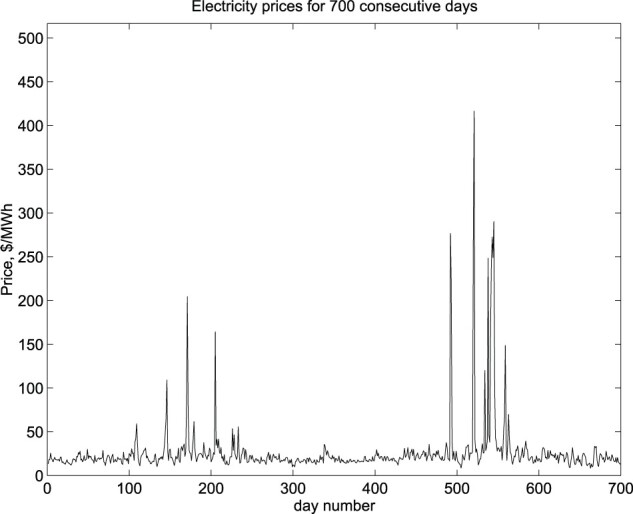
Spikes in instantaneous electricity prices during two years in the PJM (Pennsylvania–New Jersey–Maryland) energy market.

The field of change-point analysis is well studied over the last 70 years or so [33]. Thorough surveys of proposed methods can be found in [8,27,42]. Many of the proposed tools can be applied to the analysis of transient changes; for example, [18] evaluates performance of the Page's CUSUM procedure [25,26] for transient changes of a known duration. As we show, the transient change-point analysis is a different problem; in particular, the likelihood-ratio testing for a transient change is related to the maximum value of a CUSUM process.

We start with the retrospective (off-line, non-sequential) analysis of one transient change. Our goals focus on testing occurrence of a change and estimating its starting and ending moments. The level α likelihood-ratio test is derived, which leads to the maximum likelihood estimation of the interval of change. Then, we derive the asymptotic distribution of the maximum likelihood estimator.

In the case of Normal distributions, our estimator of the end of a transient segment coincides with the test statistic of [46, Section 2.2] and [35, Section 3.6]. A number of other tests are presented in [46] for a transient change in a sequence of Normal random variables. A short survey of other tests is given in [1, Section 1].

We then generalize our method to the situation of multiple transient changes. A number of algorithms have been proposed for multiple change-points that are not transient. One can use an overall maximum likelihood estimation procedure [14], although without a restriction it tends to produce false alarms. To limit false alarms, one can restrict the number of change-points or the distance between them, as in [22]. Alternatively, one can utilize binary segmentation [43,44] and wild binary segmentation [12,13], the isolate-detect scheme [2], Bayesian recursion [11] and its regression version [31], scan statistics [10], and other methods.

Building upon our analysis of one transient change, we utilize a fully sequential scheme of [3] to detect and estimate multiple transient changes. In other words, a retrospective problem that arises from a sample of a fixed size n is being solved sequentially, where change-points are detected sequentially, one at a time.

Several sequential statistical methods have been proposed for the analysis of transient changes. Under the assumption of a known duration of the post-change period, the standard CUSUM algorithm for change-point detection is modified and optimized in [15,16,41]. The optimality is understood as the lowest probability of missing a transient change [15,16] or the highest probability of detection [41], subject to the given probability of a false alarm within the given time. The optimized detection rule is the window-limited CUSUM, or WL-CUSUM. The special case of changes in the mean is considered in [24], where an approximate expression for the average run length to false alarm is given for the moving-average sum (MOSUM) algorithm.

When the assumption of a completely known duration of the period of change is not realistic, one may consider it random, put a prior distribution on each change-point, and consider the resulting Bayesian problem, as in [6,28,40].

For a more detailed overview of literature on Bayesian and non-Bayesian transient change-point detection methods, see [9,16,46].

In this work, we focus on the detection of transient changes and estimation of change-points when the change intervals are completely unknown. The considered scenarios are retrospective, in which a fixed-length data sequence is already collected, and it may contain one or more transient changes that we aim to detect without an option of requesting more data.

Existence of two alternating distributions, regarded as ‘in-control’ and ‘out-of-control’ states, leads us to a new problem of a simultaneous control of the false alarm and the false re-adjustment rates.

The new results include simultaneous control of these rates in the case of one transient change, their familywise control in the case of multiple transient changes, and the asymptotic distribution of the maximum likelihood estimator of the interval of change. Notably, our introduced threshold for α-testing of one transient change, is extended to the case of multiple transient changes, providing α-control of both familywise error rates without a Bonferroni-type correction or another adjustment for multiple comparisons. The Doob's maximal inequality, used in the derivation of this threshold, appears sufficient to guarantee familywise control regardless of the number of transient changes.

Algorithms for the detection, estimation, and testing of one transient change are derived in Section 2, and for multiple transient changes in Section 4, where the number of changes may be known or unknown. The proposed detection method, a self-correcting CUSUM procedure, is shown to detect transient changes while controlling the familywise false alarm rate and the familywise false re-adjustment rate simultaneously at the pre-determined levels. Asymptotic results are derived in Section 3. Section 5 contains illustrations and simulation results.

2. Estimation and testing of one transient change interval

In this section, we assume at most one interval of change and derive the transient change detection scheme that controls the probability of a false alarm at a pre-chosen level α. Two scenarios are possible - either all the data follow the base distribution,

$$\begin{array}{r}{H}_0:X_1,\dots ,X_n\sim F,\end{array}$$

or there is one region of change $[a,b]$, so that

$$\begin{array}{r}{H}_1:\{\begin{array}{lll}{X}_1,\dots ,X_a& \sim & F\\ X_{a+1},\dots ,X_b& \sim & G\\ X_{b+1},\dots ,X_n& \sim & F\end{array}\end{array}$$

where a and b are unknown change-points while the distributions F and G are known. The former case can be viewed as the no-change null hypothesis $H_0$, and the latter as the transient-change alternative $H_1$.

The goals are [1] to distinguish between $H_0$ and $H_1$ with a given level of significance, and [2] to estimate change-point parameters a and b in the case of $H_1$.

2.1. Maximum likelihood estimation

From now on, we assume independent observations $X_1,\dots ,X_n$. (The case of dependent data is usually solved by representing the joint likelihood function as a product of conditional densities, given past observations. Probability results will then require additional assumptions.) For the parameter $(a,b)$, the log-likelihood function is written as

$$\begin{array}{rl}L(X;a,b)& =\sum _{i=1}^a\log f\left(X_i\right)+\sum _{i=a+1}^b\log g\left(X_i\right)+\sum _{i=b+1}^n\log f\left(X_i\right)\\ & =\sum _{i=a+1}^b\log \frac{g\left(X_i\right)}{f\left(X_i\right)}+\sum _{i=1}^n\log f\left(X_i\right)\\ & =S_b-S_a+\text{const},\end{array}$$ (1)

where f and g are probability densities of distributions F and G with respect to a reference measure μ;

$$\begin{array}{r}{S}_t=\sum _{i=1}^t\log \frac{g\left(X_i\right)}{f\left(X_i\right)}=\sum _{i=1}^t{z}_i\end{array}$$

is a random walk built on marginal log-likelihood ratios $z_i$ as its increments; and $\sum _{i=1}^n\log f\left(X_i\right)$ is a constant term as it does not depend on the unknown parameters a and b. Measures F and G are not required to be mutually absolutely continuous, so that the log-likelihood ratio $\log \left(g/f\right)$ assumes values in $\overline{\mathbb{R}}=[-\mathrm{\infty },\mathrm{\infty }]$.

Maximizing  (1), we immediately obtain the maximum likelihood estimator (MLE)

$$\begin{array}{r}(\hat{a},\hat{b})=({\hat{a}}_n,{\hat{b}}_n)=\underset{a\le b}{\mathrm{a}\mathrm{r}\mathrm{g}\mathrm{m}\mathrm{a}\mathrm{x}}(S_b-S_a).\end{array}$$ (2)

Naturally, the log-likelihood (1) and the maximizer (2) are functions of the sample size n. To simplify notations, n will often be omitted, except for the asymptotic study in Section 3.4, exploring the distribution of (2) as $n\to \mathrm{\infty }$.

According to (2), the MLE returns the interval of the largest growth of random walk $S_t$. A direct method of calculating $\hat{a}$ and $\hat{b}$ can be proposed in terms of the associated cumulative-sum (CUSUM) process

$$\begin{array}{r}{W}_t=S_t-\underset{i\le t}{min}{S}_i,\end{array}$$ (3)

which vanishes at every successive point of minimum of $S_t$. Given $\hat{b}$, one finds $\hat{a}$ by minimizing $S_t$ for $t\le \hat{b}$, that is, finding the most recent zero of the CUSUM $W_t$. Then, the CUSUM does not return to zero between $\hat{a}$ and $\hat{b}$, and therefore,

$$\begin{array}{r}{S}_{\hat{b}}-S_{\hat{a}}=W_{\hat{b}}-W_{\hat{a}}=W_{\hat{b}}.\end{array}$$ (4)

Maximizing (4), we obtain its computational formula for the MLE,

$$\begin{array}{r}\hat{b}={\hat{b}}_n=\underset{0<t\le n}{\mathrm{a}\mathrm{r}\mathrm{g}\mathrm{m}\mathrm{a}\mathrm{x}}{W}_t,\hat{a}={\hat{a}}_n=max\left\{\text{Ker}\right(W)\cap [0,\hat{b}\left)\right\},\end{array}$$ (5)

where Ker $\left(W\right)=t:W_t=0$ denotes the CUSUM's ‘kernel’, or the set of its zeros.

Our estimator $\hat{b}$ matches the Levin-Kline statistic [3] of [23], which is applied to the case of Normal distributions in Section 3.6 of [35] and Section 2.2 of [46].

As an illustration, an example of a log-likelihood ratio based random walk $S_t$, the associated CUSUM process $W_t$, and the resulting transient change-point estimator $(\hat{a},\hat{b})$ is shown in Figure 2.

Figure 2.

Maximum likelihood estimation of a single transient change interval. The likelihood-ratio test statistic Λ is the largest increment of both processes $S_t$ and $W_t$.

2.2. Testing appearance of a transient change

The largest increment (4) of the random walk $S_t$ also serves as the log-likelihood ratio test statistic

$$\begin{array}{r}\mathrm{\Lambda }={\mathrm{\Lambda }}_n=\log \frac{\underset{a<b}{max}\left\{f\right(X_{0:a}\left)g\right(X_{a:b}\left)f\right(X_{b:n}\left)\right\}}{f\left(X_{0:n}\right)}=\underset{a<b}{max}(S_b-S_a)=W_{\hat{b}}\end{array}$$

for testing the no-change null hypothesis against an alternative hypothesis that a transient change occurred in our data,

$$\begin{array}{r}{H}_0:X_{0:n}\sim F\text{ vs. }{H}_1:\{\begin{array}{lll}{X}_{0:a}& \sim & F\\ X_{a:b}& \sim & G\\ X_{b:n}& \sim & F\end{array}\text{ for some }a<b,\end{array}$$

where ${\mathit{X}}_{k:m}=(X_{k+1},\dots ,X_m)$ for any k<m, and $F\left({\mathit{X}}_{k:m}\right)$ and $G\left({\mathit{X}}_{k:m}\right)$ denote joint distributions.

The likelihood-ratio test (LRT) rejects $H_0$ in favor of $H_0$ if $\mathrm{\Lambda }\ge h$ for some threshold h. The choice of h controls the balance between probabilities of Type I and Type II errors, or in other words, between the detection sensitivity and the rate of false alarms.

In order to control the probability of a false alarm at the given level α, we take advantage of the Doob's Maximal Inequality (for example, see [32], Section VII-3; [38], Section 7.1.1). It states that for a submartingale $\left\{Y_t\right\}$ and any constant $c\ge 0$,

$$\begin{array}{r}\mathbb{P}\{\underset{0\le t\le n}{sup}{Y}_t\ge c\}\le \frac{\mathbb{E}\left(Y_n^{+}\right)}{c},\end{array}$$

where $x^{+}=max\{x,0\}$.

The Doob's inequality can be applied directly to the LRT statistic

$$\begin{array}{r}\mathrm{\Lambda }=W_{\hat{b}}=\underset{0\le t\le n}{max}{W}_t\end{array}$$

in the following way. The CUSUM process (3) admits a recursive representation

$$\begin{array}{r}{W}_0=0,W_{t+1}=max\{0,W_t+z_{t+1}\}\end{array}$$

with $z_i=\log \frac{g\left(X_i\right)}{f\left(X_i\right)}$ ([25], Section 2.2). Similarly, $U_t=\exp \left\{W_t\right\}$ can be expressed recursively as

$$\begin{array}{r}{U}_0=1,U_{t+1}=max\{1,U_t{e}^{z_{t+1}}\}.\end{array}$$ (6)

It follows that ${\mathbb{E}}_F|U_t|<\mathrm{\infty }$ for every t, because

$$\begin{array}{rl}1& \le {\mathbb{E}}_F(e^{z_1}\vee 1)={\mathbb{E}}_F\{e^{z_1};z_1\ge 0\}+{\mathbb{P}}_F\{z_1<0\}\le {\mathbb{E}}_F{e}^{z_1}+1\\ & =\int \frac{g}{f}f\mathrm{d}\mu +1=1+1=2,\end{array}$$

and therefore,

$$\begin{array}{r}1\le {\mathbb{E}}_F\left(U_t\right)\le {\mathbb{E}}_F^t(e^{z_1}\vee 1)\le 2^t<\mathrm{\infty }.\end{array}$$

Also, from (6),

$$\begin{array}{r}{\mathbb{E}}_F\{U_{t+1}|U_1,\dots ,U_t\}\ge U_t{\mathbb{E}}_F{e}^{z_{t+1}}=U_t,\end{array}$$

showing that $U_t$ is a submartingale. Applying the Doob's maximal inequality to the process $\left\{U_t\right\}$, we have

$$\begin{array}{rl}\mathbb{P}\left\{\text{ Type I error }\right\}& ={\mathbb{P}}_F\{\mathrm{\Lambda }\ge h\}={\mathbb{P}}_F\{\underset{0\le t\le n}{max}{W}_t\ge h\}={\mathbb{P}}_F\{\underset{0\le t\le n}{max}{U}_t\ge e^h\}\end{array}$$ (7)

$$\begin{array}{rl}& \le e^{-h}{\mathbb{E}}_F\left(U_n\right)=e^{-h}{\mathbb{E}}_F\left(e^{W_n}\right).\end{array}$$ (8)

Thus, setting the threshold at

$$\begin{array}{r}{h}_{\alpha }=-\log \frac{\alpha }{{\mathbb{E}}_F\left(e^{W_n}\right)}\end{array}$$ (9)

guarantees the probability of a false alarm no higher than α.

A large-sample, large-threshold asymptotic expression for the Type I error probability (7) is derived in [36, Theorem 2]. By comparison, (8) is an inequality, which is valid for any finite n and h.

We conclude this section summarizing the obtained results.

Proposition 2.1 Detection of a single transient segment —

For the case of at most one transient change in the interval $[0,n]$,

• (1)The maximum likelihood estimator of the interval of change $[a,b]$ is given by (2) in terms of the random walk $S_t$ and by (5) in terms of the CUSUM process $W_t$.
• (2)
  The likelihood-ratio test (LRT) rejects the no-change hypothesis if

  $$\begin{array}{r}\mathrm{\Lambda }=\underset{0\le t\le n}{max}{W}_t\ge h\end{array}$$

  for some threshold h.
• (3)Threshold $h_{\alpha }$ determined by (9) yields a level α LRT.
• (4)The change-point detection algorithm that reports a transient change at the stopping time $T_{\alpha }=min\{t:W_t\ge h_{\alpha }$} produces a false alarm with probability $\mathbb{P}\left\{\text{false alarm}\right\}\le \alpha$.

3. Precision and limiting distribution of the MLE

In this section, we assume existence of a transient interval $(a,b]$. In other words, we assume the alternative hypothesis $H_1$ and study the distribution of the maximum likelihood estimators $(\hat{a},\hat{b})$ under $H_1$. Under this condition, we study precision of the maximum likelihood estimator for the interval of change and derive its large-sample limiting distribution.

Several concepts will be introduced as building blocks in this derivation:

• –pre-likelihood estimators (PLE), defined by condition (10), weaker than the MLE, and therefore, including all MLE;
• –local likelihood estimators (LLE), defined constructively for any local point γ;
• –detection point, which belongs to the interval of change with a given probability.

3.1. Pre-Likelihood estimators

We start by introducing so-called pre-likelihood estimators (PLE). PLE satisfy the necessary (but not sufficient) conditions (10) for a pair of points to be the MLE.

To this end, introduce the direct and inverse shifted random walk processes $\{S_{\tau ,i}^{+}{\}}_{i=1}^{n-\tau }$: $S_{\tau ,i}^{+}=S_{\tau +i}-S_{\tau }$ and $\{S_{\tau ,i}^{-}{\}}_{i=1}^{\tau -1}$: $S_{\tau ,i}^{-}=S_{\tau -i}-S_{\tau }$ respectively; $S_0^{+}=S_0^{-}=0$, $S_i=S_i^{+}=S_{1,i}=$ and $S_i^{-}=S_{n,i}^{-}$, $i=1,\dots ,n$. The MLE $(\hat{a},\hat{b})$ must satisfy inequalities

$$\begin{array}{r}\begin{array}{r}{min}_i{S}_{\hat{a},i}^{-}>0,{min}_{i\le \hat{b}-\hat{a}}{S}_{\hat{a},i}^{+}>0,\\ {max}_{i\le \hat{b}-\hat{a}}{S}_{\hat{b},i}^{-}<0,{max}_i{S}_{\hat{b},i}^{+}<0.\end{array}\end{array}$$ (10)

In the sequel, any pair $(\tilde{a},\tilde{b})$ that satisfies (10) will be called a pre-likelihood estimator (PLE). The PLE conditions (10) ensure that the left-side estimate $\tilde{a}$ cannot be improved for the given right-end $\tilde{b}$ by shifting it to increase $S_{\tilde{b}}-S_{\tilde{a}}$, and similarly, the right-side estimate $\tilde{b}$ cannot be improved for the given left-end $\tilde{a}$.

PLE are directly related to MLE, because if there exists a unique PLE, it is equal to the MLE. In the next section, we find conditions for the PLE to be unique, for a sufficiently large n.

PLE can be constructed by a combination of the direct and reverse CUSUM processes, $W_t$ and $W_t^{-}$, where the reverse CUSUM process is defined as

$$\begin{array}{r}{W}_0^{-}=0,W_{n-k}^{-}=max(0,S_1^{-},\dots ,S_k^{-})-S_k^{-},k=1,\dots ,n.\end{array}$$

The direct CUSUM $W_t$ is based upon the random walk $S_t=z_1+\dots +z_t$, whereas the reverse CUSUM is built upon the random walk that starts at time n and proceeds back in time, adding increments $(-z_i)$. Any PLE can be obtained from the kernels of these CUSUM processes, defined as $K=\{t:W_t=0\}$, $K^{-}=\{t:W_t^{-}=0\}$, and $\tilde{K}=K\bigcup K^{-}$. A pair $(\tilde{a},\tilde{b})$ is a PLE if and only if $\tilde{a}<\tilde{b}$, $\tilde{a}\in K$, $\tilde{b}\in K^{-}$, and $\{i\in \tilde{K}:\tilde{a}<i<\tilde{b}\}=\mathrm{\varnothing }$.

3.2. Local likelihood estimators

In general, there may be multiple PLEs, and their number is random. To study their distribution, we define a class of local estimators $({\tilde{a}}_{\gamma },{\tilde{b}}_{\gamma })$ that are constructed around a fixed point γ,

$$\begin{array}{r}{\tilde{a}}_{\gamma }=\gamma -\arg {min}_{i\le \gamma }{S}_{\gamma ,i}^{-}\text{and}{\tilde{b}}_{\gamma }=\gamma +\arg {max}_{i\le n-\gamma }{S}_{\gamma ,i}^{+}.\end{array}$$

We call them local likelihood estimators (LLE). Every PLE coincides with an LLE with respect to any point γ inside the interval defined by this PLE.

Below, we derive the distribution of an LLE with respect to a fixed point γ. Constructed this way, LLE ${\tilde{a}}_{\gamma }$ and ${\tilde{b}}_{\gamma }$ are independent for any fixed γ. We consider the interesting case of $a<\gamma \le b$. The distribution of ${\tilde{b}}_{\gamma }$ under $b-\gamma =k\ge 0$ is the same as the distribution of MLE in the change point problem. Then

$$\begin{array}{rl}\mathbb{P}({\tilde{b}}_{\gamma }& =b)=R_{G,k}^{-}(0\left)R_{F,n-b}^{+}\right(0)\\ & \ge \exp (-{\sum }_{m=1}^{\mathrm{\infty }}{m}^{-1}({\mathbb{P}}_F({\sum }_{j=1}^m{Y}_j\ge 0)+{\mathbb{P}}_G({\sum }_{j=1}^m{Y}_j\le 0))),\end{array}$$

where

$$\begin{array}{r}\begin{array}{rl}{R}_{H,k}^{+}\left(x\right)& ={\mathbb{P}}_H(max(0,S_1^{+},\dots ,S_k^{+})<x),\\ R_{H,k}^{-}\left(x\right)& ={\mathbb{P}}_H(max(0,S_1^{-},\dots ,S_k^{-})<x),\end{array}\end{array}$$ (11)

and the random walk process $S_k$ based on the sample from a distribution H. The last inequality follows from the Spitzer's formula (see [45]) as $k,(n-b)\to \mathrm{\infty }$ [21]. Moreover [19], under r>0,

$$\begin{array}{r}\mathbb{P}({\tilde{b}}_{\gamma }=b+r)={\int }_0^{\mathrm{\infty }}{R}_{G,b-\gamma }^{-}\left(x\right)B_{F,r,n-b-r}^{+}\left(x\right)\mathrm{d}x,\end{array}$$

and under r<0,

$$\begin{array}{r}\mathbb{P}({\tilde{b}}_{\gamma }=b+r)={\int }_0^{\mathrm{\infty }}{R}_{F,n-b}^{+}\left(x\right)B_{G,-r,b-\gamma +r}^{-}\left(x\right)\mathrm{d}x,\end{array}$$

where

$$\begin{array}{r}\begin{array}{rl}{B}_{H,k,s}^{+}\left(y\right)\mathrm{d}y& ={\mathbb{P}}_H({\mathrm{a}\mathrm{r}\mathrm{g}\mathrm{m}\mathrm{a}\mathrm{x}}_{0\le i\le k+s}{S}_i=k,S_k\in [y,y+\mathrm{d}y\left)\right)\\ B_{H,k,s}^{-}\left(y\right)\mathrm{d}y& ={\mathbb{P}}_H({\mathrm{a}\mathrm{r}\mathrm{g}\mathrm{m}\mathrm{a}\mathrm{x}}_{0\le i\le k+s}(-S_i)=k,-S_k\in [y,y+\mathrm{d}y\left)\right).\end{array}\end{array}$$ (12)

The distribution of ${\tilde{a}}_{\gamma }$ can be obtained in a similar manner:

$$\begin{array}{rl}\mathbb{P}({\tilde{a}}_{\gamma }& =a)=R_{F,a}(0\left)R_{G,\gamma -a+1}^{-}\right(0)\\ & \ge \exp (-{\sum }_{m=1}^{\mathrm{\infty }}{m}^{-1}({\mathbb{P}}_G({\sum }_{j=1}^m{Y}_j\ge 0)+{\mathbb{P}}_F({\sum }_{j=1}^m{Y}_j\le 0)));\end{array}$$

$$\begin{array}{r}\mathbb{P}({\tilde{a}}_{\gamma }=a+l)={\int }_0^{\mathrm{\infty }}{R}_{G,\gamma -a+1}^{-}\left(x\right)B_{F,-l,a+l}^{+}\left(x\right)\mathrm{d}x\end{array}$$

for l<0; and

$$\begin{array}{r}\mathbb{P}({\tilde{a}}_{\gamma }=a+l)={\int }_0^{\mathrm{\infty }}{R}_{F,a}^{+}\left(x\right)B_{G,l,\gamma -a-l+1}^{-}\left(x\right)\mathrm{d}x\end{array}$$

for l>0.

Proposition 3.1

Let a, b are fixed. Then for each $r\in J=\{-b+1,\dots ,n-b\}$,

$$\begin{array}{rl}& \underset{\gamma \in (a,b]}{inf}\mathbb{P}({\tilde{b}}_{\gamma }=b+r)\\ & \ge p_r=\{\begin{array}{l}\exp (-\sum _{m=1}^{\mathrm{\infty }}\frac{1}{m}({\mathbb{P}}_F(\sum _{j=1}^m{Y}_j\ge 0,)+{\mathbb{P}}_G(\sum _{j=1}^m{Y}_j\le 0)))\text{for}r=0,\\ {\int }_0^{\mathrm{\infty }}{R}_{F,\mathrm{\infty }}^{+}\left(x\right)B_{G,-r,\mathrm{\infty }}^{-}\left(x\right)\mathrm{d}x\text{for}r<0,+.2em\\ {\int }_0^{\mathrm{\infty }}{R}_{G,\mathrm{\infty }}^{-}\left(x\right)B_{F,r,\mathrm{\infty }}^{+}\left(x\right)\mathrm{d}x\text{for}r>0,\end{array}\end{array}$$

and for each $l\in J^{\ast }=\{-a+1,\dots ,n-a\}$,

$$\begin{array}{rl}& \underset{\gamma \in (a,b]}{inf}\mathbb{P}({\tilde{a}}_{\gamma }=a+l)\\ & \ge q_l=\{\begin{array}{l}\exp (-\sum _{m=1}^{\mathrm{\infty }}\frac{1}{m}({\mathbb{P}}_G(\sum _{j=1}^m{Y}_j\ge 0)+{\mathbb{P}}_F(\sum _{j=1}^m{Y}_j\le 0)))\text{for}l=0,\\ {\int }_0^{\mathrm{\infty }}{R}_{G,\mathrm{\infty }}^{-}\left(x\right)B_{F,-l,\mathrm{\infty }}^{+}\left(x\right)\mathrm{d}x\text{for}l<0,+.2em\\ {\int }_0^{\mathrm{\infty }}{R}_{F,\mathrm{\infty }}^{+}\left(x\right)B_{G,l,\mathrm{\infty }}^{-}\left(x\right)\mathrm{d}x\text{for}l>0.\end{array}\end{array}$$

Proof.

Continuing trajectories of the random walks occurring at time k in a neighborhood of y, we conclude that the probability of reaching maximum at time k is not increased. Hence, $B_{H,k,s}^{+}\left(x\right)$, $B_{H,k,s}^{-}\left(x\right)$ are non increased in s as s>0. In a similar manner we obtain that $R_{H,s}^{+}\left(x\right)$ and $R_{H,s}^{-}\left(x\right)$ are non increased in s as s>0. The proposition follows immediately.

The right hand sides of inequalities in the last proposition for $r\ne 0$ or $s\ne 0$ are quite complicated for practical use. Approximations suitable for computation are obtained in [19].

The inequalities in Proposition 3.1 can be used immediately to get the lower bound for the cumulative probabilities,

$$\begin{array}{r}\mathbb{P}(s\le {\tilde{a}}_{\gamma }-a\le t)\ge \sum _{l=s}^t{q}_l\text{ and }\mathbb{P}(s\le {\tilde{b}}_{\gamma }-b\le t)\ge \sum _{r=s}^t{p}_r\end{array}$$ (13)

for $s\le t$ and any $\gamma \in (a,b]$, where $p_r$ and $q_l$ are given in Proposition 3.1.

3.3. Local estimation around a detection point

The next result extends (13) from fixed γ to a random point $\hat{\gamma }$, possibly dependent on data, that has a probability of falling into $(a,b]$ bounded from below. If $\mathbb{P}(\hat{\gamma }\in (a,b\left]\right)\ge 1-\alpha$, the random point $\hat{\gamma }$ will be called a detection point of level α.

An example of a level α detection point can be constructed as follows. Let $\alpha ={\alpha }_1+{\alpha }_2$, and consider the stopping time $T_{{\alpha }_1}$, defined by part 4 of Proposition 2.1. Similarly, consider the stopping time $T_{{\alpha }_2}^{-}$ that is based on the reverse CUSUM process $W_t^{-}$. If $T_{{\alpha }_1}\le T_{{\alpha }_2}^{-}$, then any point in the interval $[T_{{\alpha }_1},T_{{\alpha }_2}^{-}]$ is a detection point of level $\alpha$.

Cumulative and tail probabilities for LLE with respect to such a point $\hat{\gamma }$ are bounded from below in the following proposition.

Proposition 3.2

Let $\hat{\gamma }$ be a detection point of level α, as defined above. Then

$$\begin{array}{rl}\mathbb{P}(s\le {\tilde{a}}_{\hat{\gamma }}-a\le t)& \ge \sum _{l=s}^t{q}_l-\alpha ;\\ \mathbb{P}(s\le {\tilde{b}}_{\hat{\gamma }}-b\le t)& \ge \sum _{r=s}^t{p}_r-\alpha ,\end{array}$$

where probabilities $p_r$ and $q_l$ are given in Proposition 3.1.

Proof.

The proof is based on the Boole inequality

$$\begin{array}{r}1-\mathbb{P}\left(AB\right)=\mathbb{P}(\overline{A}\cup \overline{B})\le \mathbb{P}\left(\overline{A}\right)+\mathbb{P}\left(\overline{B}\right)\end{array}$$

that implies $\mathbb{P}\left(AB\right)\ge \mathbb{P}\left(A\right)-\mathbb{P}\left(\overline{B}\right)$. Then for any fixed a<b,

$$\begin{array}{rl}\mathbb{P}(s\le {\tilde{a}}_{\hat{\gamma }}-a\le r)& \ge \mathbb{P}(s\le {\tilde{a}}_{\hat{\gamma }}-a\le r,\hat{\gamma }\in (a,b\left]\right)\\ & \ge {inf}_{\gamma \in (a,b]}\mathbb{P}(s\le {\tilde{a}}_{\gamma }-a\le r,\gamma \in (a,b\left]\right)\\ & \ge {inf}_{\gamma \in (a,b]}\mathbb{P}(s\le {\tilde{a}}_{\gamma }-a\le r)-\alpha \ge \sum _{l=s}^t{q}_l-\alpha ,\end{array}$$

from (13). The second inequality is obtained analogously.

3.4. Asymptotic distribution of the MLE

In this section, we study the large-sample asymptotic behavior of MLE $(\hat{a},\hat{b})$ as the sample size and all homogeneous segments tend to infinity. We assume that the parameters $a=a\left(n\right)$ and $b=b\left(n\right)$ and the interval of change $D=\left[a\right(n),b(n\left)\right]$ are dependent on n, and $\mathrm{\Delta }=min\left\{a\right(n),b(n)-a(n),n-b(n\left)\right\}\to \mathrm{\infty }$ as $n\to \mathrm{\infty }$. We use the notation $\mathbb{P}\equiv {\mathbb{P}}_{(D,n)}$ for the distribution with a transient change and ${\mathbb{P}}_H$ for the case of i.i.d. random variables $X_1,\dots ,X_n$ with the common distribution function H. In particular, ${\mathbb{P}}_F\equiv {\mathbb{P}}_{(\mathrm{\varnothing },n)}$ and ${\mathbb{P}}_G\equiv {\mathbb{P}}_{(\mathcal{N},n)}$, where $\mathcal{N}=\{1,\dots ,n\}$.

Next, we define random walks $S_k=\sum _{i=1}^k{Y}_i$ and ${\tilde{S}}_k=-\sum _{i=1}^k{Y}_i$. For example, for the transient change-point detection problem, with log-likelihood ratios $Y_i=\log \frac{g}{f}\left(X_i\right)$, the random walk $S_k$ is used to detect a change from F to G whereas ${\tilde{S}}_k$ is used to detect a change from G to F.

Let $W_k$, ${\tilde{W}}_k$ be the corresponding CUSUM processes, where $W_0={\tilde{W}}_0=0$, $W_k=S_k-\underset{i\le k}{min}{S}_i=(W_{k-1}+Y_k)\vee 0$, and ${\tilde{W}}_k=\underset{i\le k}{max}{S}_i-S_k=({\tilde{W}}_{k-1}-Y_k)\vee 0$.

We start with the following auxiliary results.

Lemma 3.3

Let ${\mathbb{E}}_{F}Y=c_1<0$. Then for any $ϵ>0$

$$\begin{array}{r}{\mathbb{P}}_F({sup}_{n\ge m}{max}_{j\le n}{W}_j/n>ϵ)\to 0\text{as}m\to \mathrm{\infty }.\end{array}$$

Proof.

Let $\mathbb{F}=\{{\mathcal{F}}_k{\}}_{k\in \mathbb{N}}$ be the natural filtration associated with the process $Y_1,Y_2,\dots$; and ${\tau }_1,{\tau }_2,\dots$ be the successive zeroes of the CUSUM process $\{W_k{\}}_{k\in \mathbb{N}}$.

Introduce $Y_k^{\ast }=Y_{k}1{\mathrm{I}}_{\{Y_k\ge 0\}}$ and $S_k^{\ast }=\sum _{j=1}^k{Y}_j^{\ast }$, $k\in \mathbb{N}$. Note that ${\mathbb{E}}_F{Y}_k^{\ast }=c_2<\mathrm{\infty }$. By the Markov property of the random process $\{S_k^{\ast }{\}}_{k\in \mathbb{N}}$: $S_k^{\ast }=\sum _{j\le k}{Y}_j^{\ast }$ with respect to the filtration $\mathbb{F}$ using Wald's identity, we obtain that ${\mathbb{E}}_F{S}_{{\tau }_k}^{\ast }={\mathbb{E}}_F{S}_{{\tau }_1}^{\ast }=c_2{\mathbb{E}}_F{\tau }_1$ for all k>1.

Let $Z_1,Z_2,\dots$ be independent copies of the random variable $S_{{\tau }_1}^{\ast }$. Then

$$\begin{array}{r}{\mathbb{P}}_F({max}_{j\le n}{W}_j/n>ϵ)\le {\mathbb{P}}_F({max}_{j\le n}{Z}_j/n>ϵ).\end{array}$$ (14)

Denote, $H\left(u\right)={\mathbb{P}}_F(Z_1\le u)$ is the distribution function of Z's. Note that the events $\{{max}_{j\le n}{Z}_j/n>ϵ\}$, $n\in \mathbb{N}$, occur infinitely many times iff the events $\{Z_k>kϵ\}$, $k\in \mathbb{N}$, occur infinitely many times; ${\mathbb{P}}_F(Z_k>kϵ)=1-H\left(kϵ\right)$. By the Borel–Cantelli lemma and Maclaurin–Cauchy test, ${\mathbb{P}}_F$ almost sure $Z_k\le kϵ$ under a sufficiently large k if

$$\begin{array}{r}{\int }_0^{\mathrm{\infty }}(1-H(xϵ\left)\right)\mathrm{d}x=\mathbb{E}{Z}_1<\mathrm{\infty }.\end{array}$$

The lemma is proved.

The next lemma follows immediately from the strong law of large numbers (SLLN) and Lemma 3.3.

Lemma 3.4

Let ${\mathbb{E}}_{F}Y=c_1<0$, ${\mathbb{E}}_{G}Y=c_2>0$ and $lim\underset{n\to \mathrm{\infty }}{inf}\frac{{\mathrm{\Delta }}_n}{n}\ge ϵ$ for some $ϵ>0$. Then

$$\begin{array}{r}\underset{r\to \mathrm{\infty }}{lim}\underset{n\to \mathrm{\infty }}{lim}\mathbb{P}(|{\hat{a}}_n-a|\ge r)=0;\underset{r\to \mathrm{\infty }}{lim}\underset{n\to \mathrm{\infty }}{lim}\mathbb{P}(|{\hat{b}}_n-b|\ge r)=0.\end{array}$$

Proof.

For the most distant from a version of the PLE ${\tilde{a}}_n$ we can write that

$$\begin{array}{rl}\mathbb{P}(a-{\hat{a}}_n\ge r)& \le \mathbb{P}(a-{\tilde{a}}_n\ge r)=\mathbb{P}({sup}_{k\le a-r}{W}_k={sup}_{k\le n}{W}_k)\\ & \le {\mathbb{P}}_F({inf}_{r\le k\le a}{\tilde{S}}_k\le 0)+\mathbb{P}({sup}_{k\le a}{W}_k\ge S_{a,b-a})\end{array}$$

where

$$\begin{array}{rl}& {\mathbb{P}}_F({inf}_{r\le k\le a}{\tilde{S}}_k\le 0)\le {\mathbb{P}}_F({inf}_{k\ge r}{\tilde{S}}_k\le 0)\\ & ={\mathbb{P}}_F({sup}_{k\ge r}{S}_k\ge 0)={\mathbb{P}}_F\left({sup}_{k\ge r}\right(S_k/k-c_1)\ge -c_1)\to 0\end{array}$$ (15)

as $r\to \mathrm{\infty }$. Moreover, for any $\delta >0$,

$$\begin{array}{r}\mathbb{P}({sup}_{k\le a}{W}_k\ge S_{a,b-a})\le {\mathbb{P}}_F({sup}_{k\le a}{W}_k>a\delta )+{\mathbb{P}}_G(S_{b-a}\le a\delta ).\end{array}$$

The first term in the right-hand side of the last inequality tends to 0 as $n\to \mathrm{\infty }$ by Lemma 3.3, and the second term tends to 0 as $n\to \mathrm{\infty }$ by the law of large numbers since $lim\underset{n\to \mathrm{\infty }}{sup}a/(b-a)\le {ϵ}^{-1}$ and $c_2>0$.

Analogously, we obtain that $\mathbb{P}({\hat{b}}_n-b\ge r)\to 0$ as $r\to \mathrm{\infty }$.

Let $ϵ>0$; $r_{ϵ}$ and $n_{ϵ}$ are such that

$$\begin{array}{r}\mathbb{P}({\hat{b}}_n-b>r_{ϵ})\le ϵ/2\end{array}$$

for all $n\ge n_{ϵ}$. Since ${\hat{a}}_n\le {\hat{b}}_n$, on the event $A_{ϵ}=\{{\hat{b}}_n-b\le r_{ϵ}\}$,

$$\begin{array}{r}\mathbb{P}({\hat{a}}_n-a\ge r)\le {\mathbb{P}}_G(\underset{r\le k\le b-a}{sup}{S}_k\le 0)+\mathbb{P}(S_{a,b-a}-\underset{k\le r_{ϵ}}{min}{S}_{b-a,k}\ge 0).\end{array}$$ (16)

The first term in the right hand side of the last inequality is tended to 0 as $r\to \mathrm{\infty }$ uniformly in $n\ge 1$ as in (15). Then there exists an $r_{0ϵ}$, such that ${\mathbb{P}}_G(\underset{r_{0ϵ}\le k\le b-a}{sup}{S}_k\le 0)\le ϵ/4$. Finally, $\underset{k\le r_{ϵ}}{min}{S}_{b-a,k}=O_P\left(1\right)$, and, therefore,

$$\begin{array}{r}\mathbb{P}(S_{a,b-a}-\underset{k\le r_{ϵ}}{min}{S}_{b-a,k}\ge 0)=\mathbb{P}\left(S_{a,b-a}/\right(b-a)-c_2\ge -c_2+\underset{k\le r_{ϵ}}{min}{S}_{b-a,k}/(b-a\left)\right)\to 0\end{array}$$

as $b-a\to \mathrm{\infty }$. Hence, the second term in (16) is not exceed $ϵ/4$ under the sufficiently large Δ. We obtained that $\mathbb{P}({\hat{a}}_n-a\ge r_{ϵ}\vee r_{0ϵ})\le ϵ,$ under the sufficiently large Δ, and, therefore,

$$\begin{array}{r}\underset{r\to \mathrm{\infty }}{lim}\underset{\mathrm{\Delta }\to \mathrm{\infty }}{lim}\mathbb{P}({\hat{a}}_n-a\ge r)=0.\end{array}$$

Convergence $\underset{r\to \mathrm{\infty }}{lim}\underset{\mathrm{\Delta }\to \mathrm{\infty }}{lim}\mathbb{P}(\hat{b}-b_n\le r)=0$ can be obtained in the similar manner. Therefore, the lemma is proved.

Lemma 3.4 yields the following proposition.

Proposition 3.5

Let $\gamma =\lambda a+(1-\lambda )b$, $\hat{\gamma }=\lambda \hat{a}+(1-\lambda )\hat{b}$ for some $\lambda \in (0,1)$; ${\mathbb{E}}_{F}Y<0$ and ${\mathbb{E}}_{G}Y>0$. Then

$$\begin{array}{r}{\mathbb{P}}_{\theta }(\hat{a}<\gamma <\hat{b})\to 1\text{and}{\mathbb{P}}_{\theta }(a<\hat{\gamma }<b)\to 1,\end{array}$$

as $lim\underset{n\to \mathrm{\infty }}{inf}{\mathrm{\Delta }}_n/n\ge ϵ$ for some $ϵ>0$. Moreover,

$$\begin{array}{r}{\mathbb{P}}_{\theta }(max(\hat{b}-\gamma ,\gamma -\hat{a})>M)\to 1\text{and}{\mathbb{P}}_{\theta }(max(b-\hat{\gamma },\hat{\gamma }-a)>M)\to 1\end{array}$$

for any fixed M>0 for all $\theta =(a,b)$ as $lim\underset{n\to \mathrm{\infty }}{inf}{\mathrm{\Delta }}_n/n\ge ϵ$ for some $ϵ>0$.

Remark 3.1

1. Lemma 3.4 actually proves that the MLE $(\hat{a},\hat{b})$ is unique with probability tending to 1 as $n\to \mathrm{\infty }$, and if $\gamma \in (a,b)$ and $({\tilde{a}}_{\gamma },{\tilde{b}}_{\gamma })$ is the LLE with respect to some point γ, then

   $$\begin{array}{r}{\mathbb{P}}_{\theta }(\hat{a}={\tilde{a}}_{\gamma },\hat{b}={\tilde{b}}_{\gamma })\to 1\end{array}$$

   as $n\to \mathrm{\infty }$ uniformly for all $a\left(n\right),b\left(n\right):lim\underset{n\to \mathrm{\infty }}{inf}{\mathrm{\Delta }}_n/n\ge ϵ$ for some $ϵ>0$.

2. Under some known point γ between a and b, the estimation problem reduces to two separate change-point estimation problems, on the direct $i=1,\dots ,\gamma$ and the inverse $i=n,n-1,\dots ,\gamma$ sets of indices.

3. The main results can be easily extended to the case of multiple transient changes ${\mathcal{D}}_n=\bigcup _{i=1}^{J_n}(a_j,b_j]$ as ${\mathrm{\Delta }}_n=\underset{j=0,\dots ,J_{n+1}}{min}(b_j-a_j)\to \mathrm{\infty }$ as $n\to \mathrm{\infty }$, where $a_0=0$ and $a_{J_n+1}=n$.

Remark 3.1(i), together with Proposition 3.1, yield the following result, which establishes the asymptotic distribution of the MLE $(\hat{a},\hat{b})$.

Proposition 3.6

Under the conditions of Lemma 3.4, for any fixed r and l,

$$\begin{array}{rl}\underset{n\to \mathrm{\infty }}{lim}\mathbb{P}(\hat{b}& =b+r)=p_r\\ & =\{\begin{array}{l}\exp (-\sum _{m=1}^{\mathrm{\infty }}\frac{1}{m}({\mathbb{P}}_F(\sum _{j=1}^m{Y}_j\ge 0,)+{\mathbb{P}}_G(\sum _{j=1}^m{Y}_j\le 0)))\text{for}r=0,\\ {\int }_0^{\mathrm{\infty }}{R}_{F,\mathrm{\infty }}^{+}\left(x\right)B_{G,-r,\mathrm{\infty }}^{-}\left(x\right)\mathrm{d}x\text{for}r<0,\\ {\int }_0^{\mathrm{\infty }}{R}_{G,\mathrm{\infty }}^{-}\left(x\right)B_{F,r,\mathrm{\infty }}^{+}\left(x\right)\mathrm{d}x\text{for}r>0;\end{array}\\ \underset{n\to \mathrm{\infty }}{lim}\mathbb{P}(\hat{a}& =a+l)=q_l\\ & =\{\begin{array}{l}\exp (-\sum _{m=1}^{\mathrm{\infty }}\frac{1}{m}({\mathbb{P}}_G(\sum _{j=1}^m{Y}_j\ge 0)+{\mathbb{P}}_F(\sum _{j=1}^m{Y}_j\le 0)))\text{for}l=0,\\ {\int }_0^{\mathrm{\infty }}{R}_{G,\mathrm{\infty }}^{-}\left(x\right)B_{F,-l,\mathrm{\infty }}^{+}\left(x\right)\mathrm{d}x\text{for}l<0,\\ {\int }_0^{\mathrm{\infty }}{R}_{F,\mathrm{\infty }}^{+}\left(x\right)B_{G,l,\mathrm{\infty }}^{-}\left(x\right)\mathrm{d}x\text{for}l>0;\end{array}\end{array}$$

where $\sum _{r\in \mathbb{Z}}{p}_r=\sum _{l\in \mathbb{Z}}{q}_l=1$, and $R^{+}$, $R^{-}$, $B^{+}$, and $B^{-}$ are defined by (11) and (12) in the previous section. Moreover,

$$\begin{array}{r}\underset{n\to \mathrm{\infty }}{lim}\underset{I\subseteq \mathbb{Z}}{sup}\left|\sum _{r\in I}\mathbb{P}\right(\hat{b}=b+r)-\sum _{r\in I}{p}_r|=0\end{array}$$ (17)

and

$$\begin{array}{r}\underset{n\to \mathrm{\infty }}{lim}\underset{I\subseteq \mathbb{Z}}{sup}\left|\sum _{l\in I}\mathbb{P}\right(\hat{a}=a+l)-\sum _{l\in I}{q}_l|=0.\end{array}$$ (18)

Proof.

Let $p_{rn}=\underset{\gamma \in (a,b)}{inf}\mathbb{P}(\hat{b}=b+r)$ for some $\gamma \in (a,b)$ and $J=\{-b+1,\dots ,n-b\}$. Then Proposition 3.1 implies that $\sum _{r\in J}{p}_{rn}\ge \sum _{r\in J}{p}_r$. Moreover, $p_{rn}=0$ for $r\notin J$ and $\sum _{r\in J}{p}_r\to 1$ as $n\to \mathrm{\infty }$. Hence, $\underset{I\subseteq \mathbb{Z}}{sup}\underset{\gamma \in (a,b)}{inf}|\sum _{r\in I}{p}_{rn}-\sum _{r\in I}{p}_r|\to 0$ as $n\to \mathrm{\infty }$. On the other hand, let $\lambda =(a+b)/2$ and $A_{\lambda }=\{\hat{b}={\tilde{b}}_{\lambda }\}$. Then $|\mathbb{P}(\hat{b}\in I)-\mathbb{P}(\tilde{b}\in I)|=|\mathbb{P}(\hat{b}\in I,{\overline{A}}_{\lambda })-\mathbb{P}({\tilde{b}}_{\gamma }\in I,{\overline{A}}_{\lambda })|\le \mathbb{P}\left(A_{\lambda }\right)\to 0$ as $n\to \mathrm{\infty }$ uniformly on $I\subseteq \mathbb{Z}$. The convergence in (17) holds. The convergence in (18) can be obtained in a similar manner. The proposition is proved.

The quantities of the type

$$\begin{array}{r}\exp (-\sum _{m=1}^{\mathrm{\infty }}\frac{1}{m}({\mathbb{P}}_F(\sum _{j=1}^m{Y}_j\ge 0,)+{\mathbb{P}}_G(\sum _{j=1}^m{Y}_j\le 0)))\end{array}$$

that appear in the limiting distribution of MLE $\hat{a}$ and $\hat{b}$ represent probabilities for a random walk with a negative drift to stay in the negative half-plane, in the case of $\hat{b}$, and for a random walk with a positive drift to stay in the positive half-plane, in the case of $\hat{a}$. These probabilities refer back to [37], later cited by many authors including [19,34]. Corollary 8.44 of [34] specifies these precise probabilities, rephrasing the fact of staying within a negative half-plane as ∞ being the first moment of becoming positive. Our probabilities in Proposition 3.6 are for two-sided random walks, making $\hat{a}$ a minimum and $\hat{b}$ a maximum, when r = 0 and l = 0.

4. Multiple transient changes and the familywise false alarm rate

Next, we consider a possibility of multiple transient changes $[a_k,b_k]$, $k=1,\dots ,K$, where K is the number of transient change intervals. The distribution of observed data oscillates between distributions F and G, switching at unknown times, so that

$$\begin{array}{r}\begin{array}{lcccc}{X}_{0:a_1}& =& (X_1,\dots ,X_{a_1})& \sim & F\\ X_{a_1:b_1}& =& (X_{a_1+1},\dots ,X_{b_1})& \sim & G\\ X_{b_1:a_2}& =& (X_{b_1+1},\dots ,X_{a_2})& \sim & F\\ X_{a_2:b_2}& =& (X_{a_2+1},\dots ,X_{b_2})& \sim & G\\ \cdots & & \cdots & & \cdots \\ X_{b_K:n}& =& (X_{b_K+1},\dots ,X_n)& \sim & F\end{array}\end{array}$$

One interpretation of this setting is a base distribution F, when the observed process is ‘in control’, that is subject to sudden disorder times $a_k$, when it goes ‘out of control’ to a disturbed distribution G. Each disorder will eventually be followed by a ‘re-adjustment’ to the base distribution, which takes place at time $b_k$.

The goal is to detect all the changes and estimate all $\left(2K\right)$ change-points $a_k$ and $b_k$. Facing a possibility of multiple changes, we aim to control a familywise false alarm rate and a familywise false re-adjustment rate that are understood as the probability of at least one erroneously detected change-point.

In the class of multiple change-point problems, existence of two alternating distributions leads to two special forms of familywise detection errors that we aim to control.

That is, a $\left(2K\right)$-dimensional change-point parameter

$$\begin{array}{r}\{a_k,b_k{\}}_{k=1}^{k=K}=\{a_1,b_1;\dots ;a_K,b_K\}\end{array}$$

is estimated by a $2\hat{K}$-dimensional estimator

$$\begin{array}{r}\{{\hat{a}}_k,{\hat{b}}_k{\}}_{k=1}^{k=\hat{K}}=\{{\hat{a}}_1,{\hat{b}}_1;\dots ;a_{\hat{K}},b_{\hat{K}}\}.\end{array}$$

A false alarm is understood as an estimated segment $[{\hat{a}}_k,{\hat{b}}_k]$ that does not intersect with any disorder region $[a_m,b_m]$. The familywise false alarm rate will be defined as the familywise error rate in the sense of [20], the probability of at least one false alarm,

$$\begin{array}{r}\text{FAR}=\mathbb{P}\left\{{\cup }_k\left(\right[{\hat{a}}_k,{\hat{b}}_k]\cap ({\cup }_j[a_j,b_j])=\varnothing )\right\}.\end{array}$$ (19)

Similarly, we call it a false re-adjustment when the estimated ‘in control’ interval $[{\hat{b}}_k,{\hat{a}}_{k+1}]$ does not contain any in-control observations, that is,

$$\begin{array}{r}\text{FRR}=\mathbb{P}\left\{{\cup }_k\left(\right[{\hat{b}}_k,{\hat{a}}_{k+1}]\cap \left({\cup }_j\right[b_j,a_{j+1}\left]\right)=\varnothing )\right\}.\end{array}$$ (20)

We aim at controlling the familywise rates of false alarms and false adjustments at pre-chosen levels α and β, respectively,

$$\begin{array}{r}\text{FAR}\le \alpha ,\text{and}\text{FRR}\le \mathrm{\text{β}}.\end{array}$$

We consider two situations, when the number of transient changes K is known or unknown.

4.1. Known number of transient changes and MLE

The log-likelihood function of $(a_k,b_k),k=1,\dots ,K$ is written as

$$\begin{array}{r}L(X;\{(a_k,b_k)\left\}\right)=\sum _{k=1}^K\sum _{i=a_k+1}^{b_k}\log \frac{g\left(X_i\right)}{f\left(X_i\right)}\end{array}$$

Maximizing it, we obtain the maximum likelihood estimator

$$\begin{array}{r}\left\{\right({\hat{a}}_k,{\hat{b}}_k){\}}_{k=1}^{k=K}=\underset{a_1<b_1<\dots <a_k<b_K}{\mathrm{a}\mathrm{r}\mathrm{g}\mathrm{m}\mathrm{a}\mathrm{x}}\sum _{k=1}^K(S_{b_k}-S_{a_k}),\end{array}$$

which are K mutually disjoint intervals of the biggest growth of $S_t$ (Figure 3).

Figure 3.

Estimation of multiple change-points.

A computational algorithm for $\left\{\right({\hat{a}}_k,{\hat{b}}_k\left)\right\}$ can be obtained as an iteration of steps outlined in Section 1 for the single-interval case, with a few modifications.

Step 1. Apply 5 to obtain the first MLE interval that corresponds to the interval of the biggest growth of the random walk $S_t^{\left(1\right)}=S_t$ and the associated CUSUM process $W_t$,

$$\begin{array}{r}{\hat{b}}_1=\mathrm{a}\mathrm{r}\mathrm{g}\mathrm{m}\mathrm{a}\mathrm{x}{W}_t,{\hat{a}}_1=max\left\{\text{Ker}\right(W)\cap [0,\hat{b}\left)\right\}.\end{array}$$

Step 2. Apply Step 1 to the processes

$$\begin{array}{rl}{S}_t^{(2,1)}& =S_t\text{for }1\le t\le {\hat{a}}_1,\\ S_t^{(2,2)}& =-(S_t-S_{{\hat{a}}_1})\text{for }{\hat{a}}_1\le t\le {\hat{b}}_1,\\ S_t^{(2,3)}& =S_t-S_{{\hat{b}}_1}\text{for }{\hat{b}}_1\le t\le n.\end{array}$$

This results in three new intervals, $[c_1,d_1]$, $[c_2,d_2]$, and $[c_3,d_3]$. Compare $D_1=S_{d_1}-S_{c_1}$, $D_2=-(S_{d_2}-S_{c_2})$, and $D_3=S_{d_3}-S_{c_3}$, and let $D_j=max\{D_1,D_2,D_3\}$.

If j = 1 or j = 3, add the corresponding interval to the MLE, i.e. let

$$\begin{array}{r}{\hat{a}}_2=c_j\text{ and }{\hat{b}}_2=d_j.\end{array}$$

If j = 2, then let

$$\begin{array}{r}{\hat{b}}_1=c_2\text{ and }{\hat{a}}_2=d_2,\end{array}$$

replacing the previously found interval $[{\hat{a}}_1,{\hat{b}}_1]$ with two intervals, $[{\hat{a}}_1,c_2]$ and $[d_2,{\hat{b}}_1]$.

Based on the reversed log-likelihood ratios $\log \left(f/g\right)$, the process $(-S_t)$ is actually the random walk that can be used to detect a change from G to F. Thus, the found interval $[c_2,d_2]$ is a candidate for a re-adjustment period, a change back to the base distribution. When the original walk $S_t$ drops more on $[c_2,d_2]$ than it grows on $[c_1,d_1]$ or $[c_3,d_3]$, the sum of increments along the obtained intervals $[{\hat{a}}_1,{\hat{b}}_1]$ and $[{\hat{a}}_2,{\hat{b}}_2]$ is higher that on any other two intervals, and thus, they will form the MLE for K = 2.

Step k. For $k=2,\dots ,K\wedge N$ (where N is the number of intervals where the random walk $S_t$ increases), we repeat the same operations as in Step 2. In every detected interval of change, $[{\hat{a}}_j,{\hat{b}}_j]$, we find an interval of the largest drop of $S_t$. In every interval between them including $[1,{\hat{a}}_1]$ and $[{\hat{b}}_{k-1},n]$, we find an interval of the largest growth of $S_t$. Then we find the interval of the largest change among them. If it is an interval of growth between ${\hat{b}}_j$ and ${\hat{a}}_{j+1}$, we simply add it to the list of intervals of change. If it is an interval $[c,d]$ of decrease between ${\hat{a}}_j$ and ${\hat{b}}_j$, we replace the previously found $[{\hat{a}}_j,{\hat{b}}_j]$ with two intervals, $[{\hat{a}}_j,c]$ and $[d,{\hat{b}}_j]$.

An example is shown in Figure 3. At step 1, the interval of the largest growth is determined as $[{\hat{a}}_1=98,{\hat{b}}_1=263]$. At step 2, the second largest growth interval is determined as $[{\hat{a}}_2=400,{\hat{b}}_1=504]$. At step 3, the largest-growth interval with ends at c = 157 and d = 190 is found inside $[{\hat{a}}_1,{\hat{b}}_1]$. Therefore, we conclude that a re-adjustment occurred between c and d, and $[{\hat{a}}_1,{\hat{b}}_1]=[98,263]$ is now replaced with two intervals, $[98,157]$ and $[190,263]$.

4.2. Unknown number of transient changes and familywise error rates

Since the number of changes K is usually unknown, the algorithm in Section 4.1 may either miss changes or produce false alarms. As noted before, intervals of the biggest growth of the random walk $S_t$ signal transient changes. Therefore, those intervals where the increment in $S_t$ exceeds a certain threshold will serve as estimated transient change intervals.

This threshold controls the rate of false alarms. As we show below, no Bonferroni or Holm type correction is needed to control the familywise error rates. Instead, both the familywise rate of false alarms  (19) and the familywise rate of false re-adjustments  (20) can be controlled by thresholds that are independent of the true number of change-points, which can remain unknown.

The algorithm can be described as follows.

1. Introduce two CUSUM processes, renewed at a random time $T\ge 0$,

   $$\begin{array}{rl}{W}_{T,t}& =S_{T+t}-\underset{0\le i\le t}{min}{S}_{T+i}=\text{CUSUM based on }(S_{T+t}-S_T),\text{renewed at }T\\ {\tilde{W}}_{T,t}& =\underset{0\le i\le t}{max}{S}_{T+i}-S_{T+t}=\text{CUSUM based on }-(S_{T+t}-S_T),\text{renewed at }T\end{array}$$

   The CUSUM $W_{T,t}$ is set to detect the next disorder time, whereas ${\tilde{W}}_{T,t}$ is tuned to determine the next re-adjustment time. A special case of T = 0 results in the initial CUSUM processes $W_t$ and ${\tilde{W}}_t$ without any resetting.
2. To control the familywise false alarm and false re-adjustment rates at the desired levels α and β, respectively, define thresholds as

   $$\begin{array}{r}{h}_{\alpha }=-\log \left(\alpha {\mathbb{E}}_F^{-1}\right(e^{W_n}\left)\right)\mathrm{a}\mathrm{n}\mathrm{d}{\tilde{h}}_{\mathrm{\text{β}}}=-\log \left(\mathrm{\text{β}}{\mathbb{E}}_G^{-1}\right(e^{{\tilde{W}}_n}\left)\right)\end{array}$$ (21)
3. The algorithm proceeds through the data series, detecting disorders and re-adjustments at stopping times ${\tau }_k$ and post-estimating change-points $a_k$ and $b_k$ sequentially for $k=1,2,\dots ,K$ as follows,

   $$\begin{array}{rl}{\tau }_1& =inf\{t:0<t\le n,W_t\ge h_{\alpha }\},\\ {\hat{a}}_1& =max\{\text{Ker}{W}_t\cap [0,{\tau }_1\left)\right\}\\ {\tilde{\tau }}_k& ={\tau }_k+inf\{t:0<t\le n-{\tau }_k,{\tilde{W}}_{{\tau }_k,t}\ge {\tilde{h}}_{\mathrm{\text{β}}}\},\\ {\hat{b}}_k& ={\tau }_k+max\{\text{Ker}{\tilde{W}}_{{\tau }_k,t}\cap [0,{\tilde{\tau }}_k-{\tau }_k\left)\right\};\\ {\tau }_k& ={\tilde{\tau }}_{k-1}+inf\{t:0<t\le n-{\tilde{\tau }}_{k-1},W_{{\tilde{\tau }}_{k-1},t}\ge h_{\alpha }\},\\ {\hat{a}}_k& ={\tilde{\tau }}_{k-1}+max\{\text{Ker}{W}_{{\tilde{\tau }}_{k-1},t}\cap [0,{\tau }_k-{\tilde{\tau }}_{k-1}\left)\right\},\end{array}$$

   until ${\tau }_k=\mathrm{\infty }$ or ${\tilde{\tau }}_k=\mathrm{\infty }$.

By this definition of stopping times ${\tau }_k$, ${\tilde{\tau }}_k$ and change-point estimates ${\hat{a}}_k$, ${\hat{b}}_k$, each stopping time belongs to the corresponding interval of transient change that it is designed to detect, ${\hat{a}}_k<{\tau }_k\le {\hat{b}}_k$ and ${\hat{b}}_{k-1}<{\tilde{\tau }}_k\le {\hat{a}}_k$. CUSUM processes $W_t$ and ${\tilde{W}}_t$ are restarted and grounded at these times. As in the previous sections, change-points $a_k$ and $b_k$ are then estimated by the last zero points of restarted CUSUM processes $W_{{\tilde{\tau }}_{k-1},t}$ and ${\tilde{W}}_{{\tau }_k,t}$, respectively.

Proposition 4.1

The transient change-point detection and estimator scheme (i)-(iii) resulting in the estimator $\{{\hat{a}}_k,{\hat{b}}_k{\}}_{k=1}^{k=K}$ controls familywise rates of false alarms and false re-adjustments at levels

$$\begin{array}{r}\text{FAR}\le \alpha \text{and}\text{FRR}\le \mathrm{\text{β}},\end{array}$$

for any unknown number of transient changes K.

Proof.

According to the algorithm (i)-(iii), a false alarms occurs in the interval $[{\hat{a}}_k,{\hat{b}}_k)$ if all the data in this interval follow the distribution F, including the segment ${\mathit{X}}_{{\hat{a}}_k:{\tau }_k}$ that triggered the false detection at time ${\tau }_k$.

Also note that each renewed CUSUM process $W_{{\tau }_k,t}=S_{{\tau }_k+t}-\underset{0\le t\le {\tau }_k}{min}{S}_{{\tau }_k+t}$ is dominated by the original CUSUM process $W_t$ on the corresponding segment,

$$\begin{array}{r}{W}_{{\tau }_k,t}\le W_{{\tau }_k+t}.\end{array}$$

This is because the subtracted term $\underset{t\ge 0}{min}{S}_t$ in the original CUSUM process cannot exceed the corresponding minimum $\underset{0\le t\le {\tau }_k}{min}{S}_{{\tau }_k+t}$ of the renewed CUSUM.

Therefore, at least one false alarm can possibly occur only if the original CUSUM process $W_t$ exceeds the threshold $h_{\alpha }$ at least once in the interval $(0,n]$ under the distribution F. The probability of the latter event is bounded by the Doob's inequality. Similarly to  (8), obtain

$$\begin{array}{rl}\text{FAR}& \le {\mathbb{P}}_F\left\{\bigcup _k(\underset{0<t\le (b_k-{\tilde{\tau }}_{k-1}{)}^{+}}{max}{W}_{{\tau }_k,t}\ge h_{\alpha })\right\}\le {\mathbb{P}}_F\{\underset{0<t\le n}{max}{W}_t\ge h_{\alpha }\}\\ & \le e^{-h}{\mathbb{E}}_F\left(e^{W_n}\right)=\alpha ,\end{array}$$

after substituting the first expression in  (21) for $h_{\alpha }$.

The inequality $\text{FRR}\le \mathrm{\text{β}}$ is proven along the same lines, replacing the CUSUM process $W_t$ with ${\tilde{W}}_t$, and accordingly, the stopping times ${\tau }_k$ with ${\tilde{\tau }}_k$ and vice versa.

5. Experimental study

In this section, we illustrate the proposed methods and explore their detection and estimation power by a simulation study. Our considered scenarios are

1. Transient changes in the mean of a Normal distribution;

2. Transient changes in the variance of a Normal distribution;

3. Transient changes between the Normal and Laplace distributions.

In this study, we estimate the detection thresholds that yield the preset rate of false alarms $\alpha =0.05$, rate of false re-adjustments $\mathrm{\text{β}}=0.05$, evaluate the detection power of the proposed methods, and assess the accuracy of change-point estimators. Familywise rates are controlled at levels $\alpha =\mathrm{\text{β}}=0.05$ in the case of multiple transient changes.

The symmetric case of changes in the mean appears quite different from the asymmetric situation of changes in the variance, where it appears more difficult to detect a variance reduction than a variance increase. Scenario [3] is interesting from a practical point of view. The Standard Normal distribution and the Laplace (Double Exponential) distribution with the location parameter $\mu =0$ and the scale parameter $b=1/\sqrt{2}$ are both symmetric, with the same zero means and the same unit variances. However, the Laplace distribution has heavier tails resulting in higher probabilities of large deviations. In industrial manufacturing, for example, large deviations may imply overheating, overcooling, a lack or an excess of a chemical ingredient. Timely detection of such changes and accurate estimation of their locations are critical parts of the quality control, because the items produced during the transient change interval are likely to be non-conforming. The use of likelihood ratios (for example, instead of Shewart charts) allows to detect such changes.

5.1. Detection and estimation of change points

Table 1 contains the probability of detection, as well as means and standard deviations of change-point estimates $\hat{a}$ and $\hat{b}$. An observed sample of size n = 1000 is assumed, with a transient change between a = 500 and b = 700. The considered scenarios include a change from the Standard Normal base distribution to the disturbed distribution:

1. To the Normal distribution with mean μ and unit variance (change in the mean);

2. To the Normal distribution with mean 0 and variance ${\sigma }^2$ (change in the variance);

3. To the Laplace distribution with mean 0 and variance 1 (change neither in the mean nor in the variance).

Table 1.

Detection thresholds, detection probabilities, and properties of change-point estimates for transient changes in the means and in the variances of Normal distributions and from the Normal to Laplace distributions.

Disturbed distribution		Threshold	Detection probability	Accuracy of Estimation
μ	σ	h	${\mathbb{P}}_{a,b}(\mathrm{\Lambda }\ge h)$	$\mathbb{E}\left(\hat{a}\right)$	$\mathrm{S}\mathrm{t}\mathrm{d}\left(\hat{a}\right)$	$\mathbb{E}\left(\hat{b}\right)$	$\mathrm{S}\mathrm{t}\mathrm{d}\left(\hat{b}\right)$
0.05	1	2.65	0.109	351.2	238.0	694.5	238.5
0.10	1	4.16	0.212	404.0	208.9	690.9	209.9
0.15	1	5.02	0.394	444.5	171.2	691.0	174.8
0.20	1	5.60	0.618	472.1	127.8	695.3	133.8
0.25	1	6.03	0.804	487.5	92.0	697.7	97.6
0.30	1	6.35	0.915	495.6	64.6	699.6	68.0
0.35	1	6.62	0.969	498.2	45.8	700.4	46.9
0.40	1	6.84	0.991	499.8	32.7	700.4	32.9
0.60	1	7.45	1	500.0	14.1	700.1	14.1
0.80	1	7.80	1	499.9	7.9	700.0	7.9
1.00	1	8.00	1	500.0	5.1	700.0	5.0
0	0.50	8.20	1	498.4	5.4	701.6	5.5
0	0.75	6.92	0.989	494.7	32.6	704.8	34.1
0	0.90	5.01	0.355	430.2	171.8	701.2	175.4
0	0.95	3.41	0.137	361.2	222.6	703.6	223.9
0	1.05	3.33	0.146	385.7	230.7	678.7	232.4
0	1.10	4.73	0.362	447.8	181.3	681.2	185.5
0	1.25	6.22	0.950	502.9	55.1	693.9	58.2
0	1.50	6.95	1	503.4	15.7	696.9	15.8
0	2.00	7.25	1	501.6	5.6	698.4	5.6
Laplace(0, $1/\sqrt{2}$)		6.4	0.975	499.9	45.7	698.1	47.4

Threshold $h_{\alpha }$ is calculated as the 95-th empirical percentile of the distribution of $\mathrm{\Lambda }=\underset{0\le t\le n}{max}\left(W_t\right)$, that yields the rate of false alarms $\text{FAR}=\alpha =0.05$. Results are based on $N=$50,000 Monte Carlo runs, and the threshold is estimated from $N_h=$200,000 Monte Carlo runs. Experimentally, we observed that estimation of the CUSUM's exponential moment ${\mathbb{E}}_F\left(e^{W_n}\right)$ for threshold 9 is less reliable due to a very high variance of $e^{W_n}$.

As one would anticipate, the detection power, expressed as the probability of detection, monotonically increases with the magnitude of change. When the transient change lasts for b−a = 200 observations, it is detected with the probability of 0.95 or higher when the mean drifts by 0.3+ standard deviations or when the standard deviation changes by 25%, in one or the other direction. Accordingly, the accuracy of estimators $\hat{a}$ and $\hat{b}$ improves with the magnitude of change resulting in lower standard errors. Results imply that the change-point estimators are nearly unbiased and distribution-consistent, converging in probability to the corresponding parameters, as the change grows in magnitude (unlike the standard notion of consistency related to large samples, see [4]).

5.2. Power analysis and the choice of a threshold

Table 2 shows power analysis for certain types of changes. The power, represented by the detection probability in change-point analysis, is estimated as a function of the magnitude and duration of transient change. Naturally, the difficulty in detecting small changes can be compensated by a sufficiently long interval where the data follows the new distribution. Even a 0.2σ change in the mean or a 10% shift in the standard deviation are quite likely to be detected, when the change sustains for a block of, say, b−a = 400 observations. A change from the Normal to the Laplace distribution with the same mean and the same variance has a 99% chance to be detected if the region of change lasts for about 250 observations.

Table 2.

Power analysis. Detection probabilities as functions of magnitude and duration of a transient change.

Change		Duration of the transient period Δ
From N(0,1) to N(μ,1)	μ	50	100	150	200	250	300	350	400	450	500
	0.1	0.068	0.102	0.152	0.213	0.281	0.346	0.394	0.465	0.532	0.571
	0.2	0.113	0.259	0.457	0.611	0.740	0.828	0.889	0.924	0.949	0.968
	0.3	0.216	0.567	0.808	0.916	0.968	0.983	0.992	0.997	0.999	1
	0.4	0.421	0.839	0.964	0.992	0.998	0.999	1	1	1	1
	0.5	0.659	0.957	0.995	1	1	1	1	1	1	1
	0.6	0.836	0.993	1	1	1	1	1	1	1	1
	0.7	0.937	0.999	1	1	1	1	1	1	1	1
	0.8	0.978	1	1	1	1	1	1	1	1	1
	0.9	0.994	1	1	1	1	1	1	1	1	1
	1.0	0.998	1	1	1	1	1	1	1	1	1
From N(0,1) to N(0,σ)	σ
	0.50	0.993	1	1	1	1	1	1	1	1	1
	0.75	0.305	0.797	0.952	0.989	0.997	0.999	1	1	1	1
	0.90	0.082	0.144	0.241	0.361	0.465	0.576	0.664	0.738	0.796	0.837
	0.95	0.062	0.084	0.108	0.142	0.171	0.211	0.254	0.290	0.330	0.357
	1.05	0.064	0.086	0.115	0.143	0.181	0.212	0.256	0.289	0.325	0.366
	1.10	0.086	0.162	0.256	0.365	0.462	0.559	0.637	0.703	0.756	0.801
	1.25	0.325	0.693	0.871	0.950	0.979	0.991	0.997	0.999	1	1
	1.50	0.865	0.992	0.999	1	1	1	1	1	1	1
	2.00	1	1	1	1	1	1	1	1	1	1
Normal to Laplace		0.323	0.731	0.905	0.973	0.991	0.997	0.999	1	1	1

A similar pattern is seen in the operating characteristic curve on Figure 4. The sensitivity-specificity ratio is represented by the probability of detection and the rate of false alarms. Easily detectable changes are represented by steeper ROC curves, which correspond to larger magnitudes of change μ and longer periods Δ of transient change. On this Figure, $\mathrm{\Delta }=10$ means that only 10 data points are observed from the changed distribution.

Figure 4.

Operating characteristics. ROC curves for change detection in the mean with various thresholds.

ROC curves can also be used for determining detection thresholds h that achieve the desired balance between the detection power and the rate of false alarms. A simple argument results in a lower bound for the needed threshold, which appears a good approximation of h for larger changes. Indeed, one large increment $z_i$ is sufficient for exceeding the threshold and triggering a false alarm, under the base distribution.

Let $F_z$ be the cumulative distribution function of the individual log-likelihood ratios $z_i=\log \left(g\right(X_i\left)/f\right(X_i\left)\right)$ under the base distribution F. The false alarm rate must be bounded from below by the probability of having at least one increment $z_i$ alone, $1,\dots ,n$, exceeding the threshold, and consequently, driving the whole CUSUM process over h. That is,

$$\begin{array}{r}\text{FAR}\ge \mathbb{P}\{\bigcup _{i=1}^n{z}_i\ge h=1-F_z^n(h\left)\right\}\end{array}$$

exceeds α if and only if $h<F_z^{-1}\left(\right(1-\alpha {)}^{1/n})$. Hence, we obtain the lower bound for the required threshold,

$$\begin{array}{r}h\ge F_z^{-1}\left(\right(1-\alpha {)}^{1/n}).\end{array}$$

For example, in case of a change in the mean of a Normal distribution, the base distribution of log-likelihood ratios $z_i$ is Normal with mean $(-{\mu }^2/2)$ and variance ${\mu }^2$. Hence,

$$\begin{array}{r}\text{FAR}\ge 1-{\mathrm{\Phi }}^n\left(\frac{h+{\mu }^2/2}{\mu }\right),\end{array}$$

and we obtain that any threshold satisfying

$$\begin{array}{r}h\ge \mu {\mathrm{\Phi }}^{-1}\left(\right(1-\alpha {)}^{1/n})-\frac{{\mu }^2}{2}\end{array}$$ (22)

yields the false alarm rate controlled at a level not exceeding α, where Φ denotes the Standard Normal c.d.f.

As seen in Figure 5,  (22) is a pretty accurate approximation of the required threshold for mean changes that are larger than 4 standard deviations. It means that detecting a change between substantially different distributions, a false alarm is likely to be cause by one extreme observation.

Figure 5.

Lower bound estimation of required thresholds.

5.3. Detection of multiple transient changes

The next experiment focuses on multiple changes whose number is unknown. In the data stream of length n = 1000, three transient change intervals are generated, each lasting for $b_k-a_k=100$ observations, k = 1, 2, 3. Each such segment is marked with a mean shifted by μ standard deviations. The algorithm described in Section 4.2 is then used to detect and estimate the start and end points of all intervals of change, with thresholds determined from the empirical null distribution of the test statistic. Since the actual number of change-points is treated as unknown, the algorithm may detect either fewer or more than N = 3 intervals of change.

In this study, we estimate the familywise false alarm rate FAR and the familywise false re-adjustment rate FRR, explore the frequency of detecting the correct and the incorrect number of changes, and evaluate the accuracy of all change-point estimators $({\hat{a}}_k,{\hat{b}}_k)$.

Results in Table 3 show that rather low familywise false alarm and false re-adjustment rates for all shifts μ; they are controlled by properly selected detection thresholds.

Table 3.

Analysis of multiple transient changes. Familywise false alarm and false re-adjustment rates and the distribution of detected intervals of change.

Shift	Threshold			Probability of detecting k intervals
μ	h	FAR	FRR	k = 0	k = 1	k = 2	k = 3	$k\ge 4$
0.1	4.14	0	0	0.77	0.23	0	0	0
0.2	5.60	0.001	0	0.44	0.49	0.07	0	0
0.3	6.36	0.002	0	0.09	0.37	0.41	0.13	0
0.4	6.84	0.007	0	0	0.07	0.36	0.56	0
0.5	7.18	0.013	0	0	0	0.11	0.87	0.01
0.6	7.44	0.020	0.002	0	0	0.02	0.96	0.02
0.7	7.64	0.024	0.003	0	0	0	0.97	0.03
0.8	7.79	0.028	0.006	0	0	0	0.97	0.03
0.9	7.94	0.027	0.008	0	0	0	0.97	0.03
1.0	8.01	0.030	0.010	0	0	0	0.96	0.04

When the sequence is observed with no change-points, the threshold explained in Section 5.1 guarantees exactly the desired rate of false alarms, subject to the Monte Carlo estimation error only. Based on the test statistic, the maximum CUSUM value, the threshold $h=h\left(n\right)$ depends on the sample size n, and it is an increasing function of n. In the presence of change-points, false alarms, if any, occur within shorter intervals between transient change segments. Shorter intervals could have been served by lower thresholds if their lengths were known. However, the duration and mere presence of transient changes is unknown, and we guarantee the desired FAR conservatively by selecting a threshold $h\left(n\right)$, which yields $\text{FAR}=\alpha$ in the absence of change-points and $\text{FAR}<\alpha$ in the presence of change-points, where the real FAR depends on the number and mutual location of transient changes, and more precisely, on the duration of each segment. The actual familywise error rates are reflected in columns 3-4 of Table 3.

Table 3 shows that for changes in the magnitude of 0.5 standard deviations or more, the multiple transient change detection algorithm is quite likely to detect precisely the correct number, K = 3 intervals of change. Small shifts are more difficult to detect. When the mean drifts away by 0.2 standard deviations or less, the procedure will almost certainly detect fewer than K transient changes. Of course, detection is more likely when a change lasts for longer than 100 observations, which can be achieved, for example, by more frequent measurements.

With the thresholds selected to control FAR and FRR, detecting more than K intervals of change is very unlikely. For K = 3, the probability of detecting more than 3 intervals is less than 0.001 for all the considered scenarios.

Accuracy of change-point estimators is evaluated in Table 4. Here, the means and standard deviations of all estimators $({\hat{a}}_k,{\hat{b}}_k)$ are calculated over those data streams that resulted in the correct number of detected intervals. Estimated means are to be compared with the actual intervals of change,

$$\begin{array}{r}[a_1,b_1]=[150,250],[a_2,b_2]=[450,550],\text{and}[a_3,b_3]=[750,850].\end{array}$$

Results suggest that change-point estimators are nearly unbiased for shifts of magnitude from about 0.4 standard deviations, with their precision visibly improving for larger shifts.

Table 4.

Analysis of multiple transient changes. Accuracy of change-point estimation.

	Means and standard deviations of change-point estimators
Shift μ	$\mathbb{E}\left({\hat{a}}_1\right)$	$\mathbb{E}\left({\hat{b}}_1\right)$	$\mathbb{E}\left({\hat{a}}_2\right)$	$\mathbb{E}\left({\hat{b}}_2\right)$	$\mathbb{E}\left({\hat{a}}_3\right)$	$\mathbb{E}\left({\hat{b}}_3\right)$	$\sigma \left({\hat{a}}_1\right)$	$\sigma \left({\hat{b}}_1\right)$	$\sigma \left({\hat{a}}_2\right)$	$\sigma \left({\hat{b}}_2\right)$	$\sigma \left({\hat{a}}_3\right)$	$\sigma \left({\hat{b}}_3\right)$
0.2	114.0	272.2	426.4	551.0	734.4	870.8	43.9	33.5	35.7	20.0	39.9	21.1
0.3	135.3	260.0	441.4	560.0	739.9	853.9	36.1	30.5	30.9	30.4	30.9	25.6
0.4	145.4	253.9	446.1	553.2	745.7	852.7	26.0	24.6	26.9	25.2	25.4	22.5
0.5	148.8	251.2	448.8	551.2	748.6	850.8	18.8	18.6	20.0	19.2	18.9	18.3
0.6	149.7	250.4	449.8	550.3	749.8	850.3	13.7	13.7	13.9	13.7	13.4	13.3
0.7	149.9	250.1	449.9	550.1	749.9	850.0	10.4	10.2	10.1	10.4	10.1	10.3
0.8	150.0	250.1	450.1	550.1	749.9	850.0	8.2	7.6	7.9	8.0	7.9	7.8
0.9	150.0	250.0	450.1	550.0	750.1	850.1	6.2	6.2	6.4	6.3	6.3	6.3
1.0	149.9	250.0	450.0	550.0	750.0	850.0	5.0	5.0	5.2	4.9	5.1	5.0

6. Summary and conclusions

The transient change-point analysis refers to temporary changes in the distribution of data. Here, we studied detection and maximum likelihood estimation of transient changes, including the cases of a single change and multiple changes, where their number may be known or unknown, and studied precision of the obtained estimators.

Even small transient changes can be detected, if they sustain for a sufficiently long period of time. The power of detection naturally reduces with smaller magnitudes or shorter durations of a change. Detection sensitivity depends on the selected threshold, which can be chosen to satisfy a preset rate of false alarms.

The next step is extension of these methods to the case of distributions with unknown (nuisance) parameters. Generalized likelihood ratios and Bayesian methods have been proposed to handle nuisance parameters in the situations of a single change. Application of similar techniques to the case of multiple transient changes will allow detecting changes from the base distribution to different disturbed distributions in each transient change interval.

Funding Statement

Research of M. Baron is supported by the NSF [grant number 1737960] and the Defense Advanced Research Projects Agency (DARPA) [grant number HR0011-18-C-0051]. Research of S. Malov is supported by the Russian Science Foundation (RSF) [grant number 20-14-00072].

Disclosure statement

No potential conflict of interest was reported by the author(s).

References

- 1.Abd-Elnaser S., Rabou A.S., and Gad A.M., Change-point rank tests with epidemic alternatives, Egypt. Stat. J. 50 (2006), pp. 114–135. [Google Scholar]
- 2.Anastasiou A. and Fryzlewicz P., Detecting multiple generalized change-points by isolating single ones, Metrika 85 (2022), pp. 141–174. [DOI] [PMC free article] [PubMed] [Google Scholar]
- 3.Baron M., Sequential methods for multistate processes, in Applied Sequential Methodologies, N. Mukhopadhyay, S. Datta, and S. Chattopadhyay, eds., Dekker, New York, 2004, pp. 55–73.
- 4.Baron M. and Granott N., Consistent estimation of early and frequent change points, in Foundations of Statistical Inference, J. Haitovsky, H. R. Lerche, and Y. Ritov, eds., Physica-Verlag, Heidelberg, New York, 2003, pp. 181–194.
- 5.Baron M., Rosenberg M., and Sidorenko N., Electricity pricing: Modeling and prediction with automatic spike detection, Energy, Power Risk Management 2001 (2001), pp. 36–39. [Google Scholar]
- 6.Baron M., Rosenberg M., and Sidorenko N., Divide and conquer: Forecasting power via automatic price regime separation, Energy, Power Risk Management 2002 (2002), pp. 70–73. [Google Scholar]
- 7.Bianchi A.M., Mainardi L., Petrucci E., Signorini M.G., Mainardi M., and Cerutti S., Time-variant power spectrum analysis for the detection of transient episodes in HRV signal, IEEE Trans. Biomed. Eng. 40 (1993), pp. 136–144. [DOI] [PubMed] [Google Scholar]
- 8.Chen J. and Gupta A.K., Parametric Statistical Change Point Analysis: With Applications to Genetics, Medicine, and Finance, Birkhäuser, Boston, MA, 2012.
- 9.Egea-Roca D., López-Salcedo J.A., Seco-Granados G., and Poor H.V., Performance bounds for finite moving average tests in transient change detection, IEEE. Trans. Signal. Process. 66 (2018), pp. 1594–1606. [Google Scholar]
- 10.Eichinger B. and Kirch C., A MOSUM procedure for the estimation of multiple random change points, Bernoulli 24 (2018), pp. 526–564. [Google Scholar]
- 11.Fearnhead P., Exact and efficient Bayesian inference for multiple changepoint problems, Stat. Comput. 16 (2006), pp. 203–213. [Google Scholar]
- 12.Fryzlewicz P., Wild binary segmentation for multiple change-point detection, Ann. Stat. 42 (2014), pp. 2243–2281. [Google Scholar]
- 13.Fryzlewicz P., Detecting possibly frequent change-points: Wild binary segmentation and steepest-drop model selection, J. Korean. Stat. Soc. 49 (2020), pp. 1027–1070. [DOI] [PMC free article] [PubMed] [Google Scholar]
- 14.Fu Y.-X and Curnow R.N., Maximum likelihood estimation of multiple change points, Biometrika 77 (1990), pp. 563–573. [Google Scholar]
- 15.Guépié B.K., Fillatre L., and Nikiforov I., Detecting a suddenly arriving dynamic profile of finite duration, IEEE Trans. Inform. Theory 63 (2017), pp. 3039–3052. [Google Scholar]
- 16.Guépié B.K., Fillatre L., and Nikiforov I.V., Sequential detection of transient changes, Seq. Anal. 31 (2012), pp. 528–547. [Google Scholar]
- 17.Gut A. and Steinebach J., A two-step sequential procedure for detecting an epidemic change, Extremes 8 (2005), pp. 311–326. [Google Scholar]
- 18.Han C., Willett P.K., and Abraham D.A., Some methods to evaluate the performance of page's test as used to detect transient signals, IEEE. Trans. Signal. Process. 47 (1999), pp. 2112–2127. [Google Scholar]
- 19.Hinkley D.V., Inference about the change-point in a sequence of random variables, Biometrika 57 (1970), pp. 1–17. [Google Scholar]
- 20.Hochberg Y. and Tamhane A.C., Multiple Comparison Procedures, Wiley, New York, 1987. [Google Scholar]
- 21.Hu I. and Rukhin A.L., A lower bound for error probability in change-point estimation, Stat. Sin. 5 (1995), pp. 319–331. [Google Scholar]
- 22.Lee C.-B., Nonparametric multiple change-point estimators, Statist. Probab. Lett. 27 (1996), pp. 295–304. [Google Scholar]
- 23.Levin B. and Kline J., The cusum test of homogeneity with an application in spontaneous abortion epidemiology, Stat. Med. 4 (1985), pp. 469–488. [DOI] [PubMed] [Google Scholar]
- 24.Noonan J. and Zhigljavsky A., Power of the MOSUM test for online detection of a transient change in mean, Seq. Anal. 39 (2020), pp. 269–293. [Google Scholar]
- 25.Page E.S., Continuous inspection schemes, Biomterika 41 (1954), pp. 100–115. [Google Scholar]
- 26.Page E.S., On problems in which a change in a parameter occurs at an unknown point, Biometrika 44 (1957), pp. 248–252. [Google Scholar]
- 27.Poor H.V. and Hadjiliadis O., Quickest Detection, Cambridge University Press, Cambridge (UK), 2009. [Google Scholar]
- 28.Repin V.G., Detection of a signal with unknown moments of appearance and disappearance, Problemy Peredachi Informatsii 27 (1991), pp. 61–72. [Google Scholar]
- 29.Rosenberg M., Bryngelson J.D., Baron M., and Papalexopoulos A.D., Transmission valuation analysis based on real options with price spikes, in Handbook of Power Systems II; Energy Systems Part I, S. Rebennack, P.M. Pardalos, M.V.F. Pereira and N. Iliadis, eds., Springer, Berlin-Heiderberg, 2010, pp. 101–125.
- 30.Rosenberg M., Bryngelson J.D., Sidorenko N., and Baron M., Price spikes and real options: transmission valuation, in Real Options and Energy Management, E.I. Ronn, ed., Risk Books, London, 2002, pp. 323–370.
- 31.Seidou O. and Ouarda T., Recursion-based multiple changepoint detection in multiple linear regression and application to river streamflows, Water. Resour. Res. 43(7) (2007). DOI: 10.1029/2006WR005021. [DOI] [Google Scholar]
- 32.Shiryaev A.N., Probability, 2nd ed. Springer-Verlag, New York, 1995. [Google Scholar]
- 33.Shiryaev A.N., Quickest detection problems: Fifty years later, Seq. Anal. 29 (2010), pp. 345–385. [Google Scholar]
- 34.Siegmund D., Sequential Analysis: Tests and Confidence Intervals, Springer-Verlag, New York, 1985. [Google Scholar]
- 35.Siegmund D., Boundary crossing probabilities and statistical applications, Ann. Stat. 14 (1986), pp. 361–404. [Google Scholar]
- 36.Siegmund D., Approximate tail probabilities for the maxima of some random fields, Ann. Probab. 16 (1988), pp. 487–501. [Google Scholar]
- 37.Spitzer F., Principles of Random Walk, Van Nostrand, New York, 1966. [Google Scholar]
- 38.Stroock D.W., Mathematics of probability, Vol. 149. American Mathematical Soc., 2013.
- 39.Tafakori L., Pourkhanali A., and Fard F.A., Forecasting spikes in electricity return innovations, Energy 150 (2018), pp. 508–526. [Google Scholar]
- 40.Tartakovskii A.G., Detection of signals with random moments of appearance and disappearance, Probl. Peredachi Inf. 24 (1988), pp. 39–50. [Google Scholar]
- 41.Tartakovsky A.G., Berenkov N.R., Kolessa A.E., and Nikiforov I.V., Optimal sequential detection of signals with unknown appearance and disappearance points in time, IEEE. Trans. Signal. Process. 69 (2021), pp. 2653–2662. [Google Scholar]
- 42.Tartakovsky A. G., Nikiforov I. V., and Basseville M., Sequential Analysis Hypothesis Testing and Change-Point Detection, Chapman & Hall/CRC, 2014. [Google Scholar]
- 43.Vostrikova L. Ju., Detecting ‘disorder’ in multidimensional random processes, Sov. Math. Dokl. 24 (1981), pp. 55–59. [Google Scholar]
- 44.Wang X., Liu B., Zhang X., and Liu Y., Efficient multiple change point detection for high-dimensional generalized linear models, Can. J. Stat. (2022). DOI: 10.1002/cjs.11721. [DOI] [PMC free article] [PubMed] [Google Scholar]
- 45.Woodroofe M., Nonlinear Renewal Theory in Sequential Analysis, SIAM, 1982. [Google Scholar]
- 46.Yao Q., Tests for change-points with epidemic alternatives, Biometrika 80 (1993), pp. 179–191. [Google Scholar]
- 47.Zhang L. and Li Y., Regime-switching based vehicle-to-building operation against electricity price spikes, Energy Econ. 66 (2017), pp. 1–8. [Google Scholar]
- 48.Zhou B., Chioua M., Bauer M., Schlake J.C., and Thornhill N.F., Improving root cause analysis by detecting and removing transient changes in oscillatory time series with application to a 1, 3-butadiene process, Ind. Eng. Chem. Res. 58 (2019), pp. 11234–11250. [Google Scholar]