Toward Automatic Inference of Glycan Linkages Using MSⁿ and Machine Learning—Proof of Concept Using Sialic Acid Linkages

Abstract

Glycosidic linkages in oligosaccharides play essential roles in determining their chemical properties and biological activities. MSⁿ has been widely used to infer glycosidic linkages but requires a substantial amount of starting material, which limits its application. In addition, there is a lack of rigorous research on what MSⁿ protocols are proper for characterizing glycosidic linkages. In this work, to deliver high-quality experimental data and analysis results, we propose a machine learning-based framework to establish appropriate MSⁿ protocols and build effective data analysis methods. We demonstrate the proof-of-principle by applying our approach to elucidate sialic acid linkages (α2′–3′ and α2′–6′) in a set of sialyllactose standards and NIST sialic acid-containing N-glycans as well as identify several protocol configurations for producing high-quality experimental data. Our companion data analysis method achieves nearly 100% accuracy in classifying α2′–3′ vs α2′–6′ using MS⁵, MS⁴, MS³, or even MS² spectra alone. The ability to determine glycosidic linkages using MS² or MS³ is significant as it requires substantially less sample, enabling linkage analysis for quantity-limited natural glycans and synthesized materials, as well as shortens the overall experimental time. MS² is also more amenable than MS^3/4/5 to automation when coupled to direct infusion or LC-MS. Additionally, our method can predict the ratio of α2′–3′ and α2′–6′ in a mixture with 8.6% RMSE (root-mean-square error) across data sets using MS⁵ spectra. We anticipate that our framework will be generally applicable to analysis of other glycosidic linkages.

Introduction

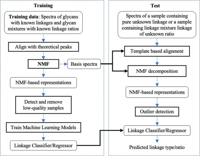
Tandem mass spectrometry (MSⁿ) has been widely used to characterize and infer glycosidic linkages. However, to obtain enough signals at the requisite MSⁿ level, it requires large quantities of starting material and additional instrumental time. Moreover, highly trained personnel are needed to conduct experiments, troubleshoot protocols, and interpret the collected data. We propose a framework (Figure 1) to deliver appropriate MSⁿ protocols for the characterization of glycosidic linkages as well as the development of machine learning techniques for the automatic inference of sialic acid–galactose linkage by analyzing collected MSⁿ data. To train the machine learning algorithm, a set of glycans with known structures and linkages was used to generate MSⁿ spectra training data sets utilizing various protocol settings and conditions. Using this data set, machine learning techniques were developed to train models to discover and recognize diagnostic MSⁿ patterns that differentiate glycosidic linkages, some of which can be too complex for humans to recognize without computer assistance. In addition, we hope machine learning can differentiate linkages at shallow MS levels as it will dramatically simplify the experimental procedure and reduce the amount of material needed, which may make it feasible to automate experiments.

Figure 1.

A machine learning-based framework for automatic inference of linkages using MSⁿ. An MSⁿ spectrum data set is collected by using glycans of known structures that contain various glycosidic linkages. (A) In the training phase, data preprocessing methods are developed to normalize raw MSⁿ spectra, detect outliers, and so on. Then, machine learning models are developed to learn representations of spectra, analyze linkage, and identify appropriate protocols for generating high-quality and informative spectra. (B) In the test phase, test spectra are first preprocessed by the data preprocessing component established in the training phase and then are fed to the machine learning models trained in the training phase to produce linkage analysis results. It is recommended that the test spectra should be generated using the MSⁿ protocol(s) identified in the training phase.

Sialic acids are a broad class of 9-carbon acidic sugars that are common moieties in an array of glycomaterials. As a terminal residue of N-linked glycans, sialic acids remain challenging to analyze for a variety of reasons. To date, more than 60 genes are known to be involved in sialic acid biology, leading to monosaccharide, positional, and linkage diversity in biological systems.¹ This diversity greatly increases the heterogeneity of biomaterials containing sialic acids, where multiple forms and linkage patterns can be present in isobaric glycoforms. In addition, the sialic acid glycosidic bond is quite labile, with several methods of analysis inadvertently resulting in the desialyation of target glycomaterials.

To develop a proof-of-principle, we focused on two common types of sialic acid linkages: α2′–3′ and α2′–6′. Many studies focused on glycosylation require multiple analytical techniques designed to separately handle sialic acid identification, composition, and linkage.²⁻⁶

Figure 2 shows a typical MSⁿ workflow, which is effective for determining sialic acid linkage (α2′–3′ and/or α2′–6′).⁷ However, this method requires collecting data up to the MS⁵ level and requires both a substantial amount of material and active user time, making this ineffective for many applications. Furthermore, numerous experimental parameters can be adjusted while collecting MSⁿ spectra, and it remains unclear which settings are appropriate for producing high-quality and reproducible data. Therefore, it is crucial to identify effective experimental settings that are applicable to other sialic acid-containing glycomaterials. This current MS⁵ experiment is unable to determine the approximate amounts of either α2′–3′ and/or α2′–6′ sialylation present. This method relies on the existence of very few MS⁵ signature ions to distinguish α2′–3′ and α2′–6′ and may overlook information carried by other fragment ions that may be useful to estimate the ratio of α2′–3′ to α2′–6′ linkage. These challenges contribute to the lack of knowledge pertaining to sialic acid glycobiology.

Figure 2.

Sialic acid linkage determination (α2′–3′ vs α2′–6′) using MS⁵. At each of the MS^2/3/4 levels, a fragment m/z (marked by an asterisk (*)) is manually decided as a precursor of the next MS level. All spectra use lithium as the ion adduct. The detection of diagnostic signatures for differentiating α2′–3′ and α2′–6′ occurs at the MS⁵ level. The fragments corresponding to the α2′–3′ and α2′–6′ MS⁵ signatures (i.e., F₁, F₂, F₃, and F₄) are shown in the box.

In this work, we aim to deliver appropriate MSⁿ workflows for characterizing sialic acid linkages (α2′–3′ and α2′–6′) and machine learning techniques and models for

• (A)differentiating sialic acid linkage type (α2′–3′ vs α2′–6′)
• (B)estimating the ratio of α2′–3′ vs α2′–6′ in samples containing mixtures of α2′–3′- and α2′–6′-linked sialic acids.

MS^2/3/4/5 spectra were collected using a set of standard sialic acid-containing glycomaterials, which were used to build linkage classifiers using machine learning. Test results show that sialic acid linkages (α2′–3′ to α2′–6′) can be robustly determined using only MS², MS³, or MS⁴ spectra. Additionally, we trained a regression model for accurately estimating the ratio between α2′–3′ and α2′–6′ in samples containing mixtures. Finally, we provide an optimized method for generating high-quality data for linkage classification/regression.

Methods

Preparation of Samples

The samples used in this experiment can be categorized into three distinct categories: sialyllactose “standard” samples, NIST standard N-glycans, and N-linked glycans released from purchased glycoprotein standards, some of which were selectively desialylated with α2′–3′-specific neuraminidase prior to release with PNGase F.

Stock solutions of α2′–3′ sialyllactose and α2′–6′ sialyllactose (Sigma-Aldrich, St. Louis, MO, USA) sugars were prepared at a concentration of 1 mg/mL in water. For the multilevel mass spectrometry experiments, five sialyllactose sample mixtures (a–e) were prepared: (a) 100% α2′–3′ sialyllactose, (b) 90% α2′–3′ sialyllactose with 10% α2′–6′ sialyllactose, (c) 50% α2′–3′ and 50% α2′–6′ sialyllactose, (d) 10% α2′–3′ sialyllactose with 90% α2′–6′ sialyllactose, and (e) 100% α2′–6′ sialyllactose. A 1 μg amount of total sugar was used for each sample, and samples were lyophilized prior to permethylation.

Six NIST standards were used from the NIST 3655 Glycans in Solution Standard Reference Material: G2S1(6), G2S2(3), G2S2(6), G2FS1(6), G2FS2(3), and G2FS2(6). No further preparation was required for these samples prior to permethylation.

N-Linked glycans were released from 100 μg of fetuin and transferrin, as previously reported,⁸⁻¹⁰ with the added step of neuraminidase treatment for select samples prior to release. Briefly, fetuin samples that were treated with α2′–3′ neuraminidase S (New England Biolabs, Cat# P0743S) were incubated with 2 μL of enzyme in ammonium bicarbonate buffer with a total reaction volume of 50 μL at 37 °C overnight. Following overnight incubation with α2′–3′ neuraminidase, the enzyme was heat inactivated at 95 °C for 5 min. Following heat inactivation, neuraminidase-treated samples and untreated glycoproteins were reduced using 25 mM dithiothreitol (DTT) and desalted using 10 kDa molecular weight cut off (MWCO) spin filters (Amicon Ultra). Glycoproteins were then incubated with 2 μL of PNGase F (New England Biolabs, Cat# P0709L) overnight at 37 °C. Released N-glycans were then isolated from the de-N-glycosylated protein using 10 kDa MWCO spin filters and further purified using a C18 SPE cartridge. Samples were lyophilized prior to permethylation.

Permethylation

Samples were permethylated as previously described.⁵ Briefly, samples were permethylated by the addition of DMSO–NaOH base and iodomethane while shaking the samples vigorously at room temperature for 15 min. The reaction was quenched with the addition of 4× volumes of water, and an aqueous–organic phase extraction was performed with the addition of dichloromethane. The aqueous layer was removed, and the organic layer was washed several times with additional water, followed by the removal and drying of the organic layer under a stream of nitrogen gas. Dried samples were resuspended in 200 μL of 50:50 methanol:water solution with 1 mM lithium carbonate for mass spectrometric analysis.

Multilevel Mass Spectrometry

Data was collected by direct infusion (1 μL/min) nanoelectrospray on a Thermo Fisher Orbitrap Eclipse Tribrid Mass Spectrometer (Thermo Fisher Scientific, Waltham, MA, USA) in positive ion mode. An applied voltage of 1900 V and an ion transfer tube temperature of 275 °C were used for data acquisition. Data was collected in profile mode. Quadrupole isolation was used with an activation Q of 0.25, and Orbitrap detection mode was used at a resolution of 120 000 for all MSⁿ levels except for MS⁵, for which ion trap detection mode was used. Fragmentation was performed using CID with the CID time set to 10 ms. The experimental parameters important for the purpose of data acquisition were isolation window and CID percentage; the isolation windows used were m/z = 1, m/z = 2, and m/z = 3, and the CID percentages that were used were 30%, 35%, 40%, 45%, and 50%. Table S1 (in Supporting Information) summarizes all MS experiments and conditions.

The fragmentation pathway for each sample was determined using GlycoWorkbench v1.1.3840. An example MS⁵ spectrum with the fragmentation pathway is shown in Figure S1. The fragmentation of the sialic acid-linked galactose at the MS⁵ level, which is necessary for α2′–3′ and α2′–6′ linkage determination, was the end product for all fragmentation pathways.¹¹ An example fragmentation pathway is shown in Figure 2. To summarize, three data sets were collected for machine learning tasks.

• (1)The University of Georgia Sialyllactose (UGA-S) Data Set: This data set comprises the mass spectra of the purchased samples containing only fragments of MS⁴. It encompasses five different α2′–3′ to α2′–6′ linkage ratios: 1:0, 0.9:0.1, 0.5:0.5, 0.1:0.9, and 0:1.
• (2)The NIST Data Set: This data set contains the MS^2/3/4/5 spectra of the NIST standard glycans: G2S2(3), G2FS2(3), G2S1(6), G2S2(6), G2FS1(6), and G2FS2(6).
• (3)The University of Georgia Released (UGA-R) Glycan Data Set: This data set contains the MS^2/3/4/5 mass spectra of released glycans extracted from biological samples: a control transferrin sample, a control fetuin sample, and an α2′–3′ neuraminidase-treated fetuin sample. This data set serves the primary purpose of testing and analyzing the model in question.

Table S2 (in Supporting Information) provides more details about the MSⁿ data sets collected in this study.

Overview of the Framework Implementation

Figure 3 illustrates our implementation of the framework (Figure 1) for building and applying the machine learning models to infer the sialic acid α2′–3′ and α2′–6′ linkages. The key components of this implementation are explained in the following sections. In the data preprocessing step of the training phase, since we know the structures of the glycans, we can align the experimental spectra with the theoretical spectra of glycans. Then, we employ non-negative matrix factorization (NMF)¹² to learn a set of basis spectra that spans the aligned experimental spectra. This step represents each experimental spectrum as a linear combination of the basis spectra, which also allows us to filter out outlier (low-quality) spectra. The NMF-based representations are later used to train machine learning models: linkage classifier for classifying linkage and linkage regressor for estimating the linkage ratio. In the data preprocessing step of the test phase, a test spectrum is aligned to the basis spectra. The derived NMF-based representation is then used to decide if the test spectrum is an outlier or not. If not, its representation is fed into the trained linkage classifier or regressor to produce a prediction. The implement was applied to build linkage classifiers at each of the MS^2/3/4/5 levels and linkage regressor at the MS⁵ level. It should be noted that this implementation is applied to each MS level independently. This allows us to pursue the goal of distinguishing linkages at lower MS levels.

Figure 3.

Implementing the framework. This diagram illustrates our implementation of the proposed framework. See the main text for detailed explanations. The training phase produces the basis spectra and linkage classifier/regressor that are applied to linkage analysis in the test phase.

Training Data Preprocessing

The raw mass spectra were converted to the mxXML format using msconvert.(13) The peaks in each scan of the MS data were extracted by using mzxml2peaks in MATLAB and were resampled to make the m/z of all scans equally spaced. The resampling resolutions for the MS², MS³, MS⁴, and MS⁵ are 23 000, 23 000, 23 000, and 10 000, respectively. In our data, each spectrum consists of 250 scans at different retention times. Each scan was aligned to its corresponding theoretical spectrum using the MATLAB msalign(14) function. The alignment of a spectrum was calculated as the mean of its aligned scans. The aligned spectra were then used in downstream analyses including spectrum representation learning, linkage classification, and linkage ratio estimation. After alignment, the spectra were log transformed to enable machine learning to capture diverse features with intensities of different scales and were also L1-normalized to reduce the effects of volume differences in the samples used to produce the data.

Learning Representations of Spectra Using NMF

We applied non-negative matrix factorization (NMF)¹² to learn representations of spectra at each MS level, which we call the basis spectra, to capture the characteristics of different linkages. NMF has been previously applied to chromatographic pattern detection,¹⁵ spectral deconvolution,¹⁶ and mass spectrometry imaging.¹⁷ In our context, NMF learns a small set of base spectra to span the training data. Mathematically, given a training spectrum set , where n is the number of spectra and m is the number of m/z readings, NMF factors X into the product of a nonnegative basis matrix and a nonnegative coefficient matrix so that the following Frobenius distance is minimized

1

Each column of the basis matrix W is a base spectrum, and each row of the coefficient matrix H specifies the coefficients for linearly combining the basis spectra to reconstruct the corresponding spectrum in X. Both W and H can be numerically estimated by the iterative procedure¹²

where × represents elementwise multiplication and fraction is also based on elements. We used nonnegative double singular value decomposition (NNDSVD)¹⁸ to initialize the base spectra. We can represent any given spectrum x by its decomposition into a linear combination of the base spectra in W as x ≈ Wh_x, where is the NMF-based representation of x and can be used in downstream tasks (e.g., linkage determination or linkage ratio estimation in our case).

In the test phase, given a test spectrum whose linkage identity is to be determined, we first align it to each of the learned basis spectra in W using msalign. The alignment score is calculated as the cosine similarity. Only peaks with relative abundance over 0.1 are used in calculating alignments. The alignment with the best score is chosen, and the NMF-based representation of the aligned spectrum is then calculated using the method described above.

Figure 4 illustrates the ability of our representation learning method to capture essential signals on the MS⁵ data. Two basis spectra were learned from the NIST data set, and they clearly encode two different patterns. One of them contains the signatures of α2′–3′ (m/z = 103.08 and 131.07), and the other contains the signatures of α2′–6′ (m/z = 89.06, 117.06). The basis spectra of other MS levels are provided in Supporting Information Figures S4–S7. We determine the number of components for the basis spectra via cross-validation (see the model evaluation section) in the following way. We tried 2, 4, 8, 16, and 32 basis spectra and obtained the best results for both the linkage classification and the regression tasks when utilizing only 2 basis spectra.

Figure 4.

MS⁵ basis spectra learned by NMF. The NIST data set is used. Two basis spectra are learned, and they align perfectly with the theoretical peaks of α2′–3′ and α2′–6′. The top basis spectrum contains the conventional α2′–3′ diagnostic signatures (m/z = 103.08 and 131.07), and the bottom basis spectrum contains the conventional α2′–6′ diagnostic signatures (m/z = 89.06, 117.06).

The learned basis spectra can serve as templates for aligning new spectra. Alignment is needed to remove systematic error/noise when analyzing mass spectra. A commonly used method is to align a new spectrum with a manually chosen library of spectra.¹⁹⁻²² The basis spectra learned by NMF span the spectrum space and hence offer a proper alternative to the manually chosen spectra. Since the number of basis spectra is small, the computational complexity of alignment is reduced significantly by replacing a spectrum library with the basis spectra.

The basis spectra also offer a means to robustly represent spectra. It is often the case that the number of training spectra is usually much smaller than the number of peaks in them. In machine learning, this is referred as the “p ≫ n” problem, where p and n indicate the numbers of predictors and samples, respectively. It can be challenging to learn a robust model when “p ≫ n”. The NMF-based representation learning explores interactions between predictors to learn a small set of base spectra and allows us to represent a spectrum as a weighted combination of the base spectra. This effectively reduces “p” in downstream tasks and enables the building of robust models.

Spectrum Outlier Detection

Spectra of low quality (i.e., outliers) can be occasionally produced in experiments. They should be detected and removed from the training set to help train a robust linkage classification/regression model. Moreover, we should also avoid generating predictions for outliers as the prediction results could be unreliable. Since the learned NMF base spectra are supposed to span the desired input space, they can be used to decide if a spectrum y is an outlier. We use the basis spectra to reconstruct y as ỹ = Wh_y, where h_y is the representation of y in the space defined by the basis spectra. The quality score of y is defined as the cosine similarity between y and its reconstruction using the basis spectra

2

A low similarity score indicates that the spectrum is likely to be an outlier. The similarity threshold should be empirically decided (see Outlier Detection in the Results section). The outlier detection was applied to test spectra to avoid producing misleading prediction results. Table S3 lists the outlier spectra detected.

Training Machine Learning Models

Linkage Classification

This task is to differentiate α2′–3′ or α2′–6′ linkages, which was treated as a binary classification problem. In instances where the sample contains both linkages, the system outputs the linkage associated with the higher probability. At each MS level, we had a training set {⟨x_i, y_i⟩}, where x_i represents NMF-learned representation of the ith spectrum and y_i ∈ {0, 1} (0 and 1 indicate α2′–3′ and α2′–6′, respectively) is the class label; we trained a model f: X → Y that takes the NMF-based representation of a spectrum as the input and decides if the spectrum is from α2′–3′ or α2′–6′. The trained model can be later applied to new spectra not in the training set. We chose support vector machine (SVM)²³ as the linkage classifier model. SVM learns a hyperplane that maximizes the separation between samples of different classes. Kernel functions can be used to allow SVM to produce nonlinearity boundaries between different classes. The radical basis function (RBF) kernel is used. Previous works have used SVMs in mass spectrometry data for predicting cancer.²⁴ The input to SVM is standardized so that every feature has a mean of 0 and a standard deviation of 1.

Linkage Regression

A sample can contain a mixture of α2′–3′ and α2′–6′ sialic acid linkages. It is important to estimate the ratio of α2′–3′- to α2′–6′-linked sialic acid in a sample; however, methods for doing so are scarce. To this end, we trained support vector regression (SVR) to predict the relative α2′–3′ abundance, i.e., (molarity of α2′–3′ sialylactose)/(molarity of α2′–3′ sialylactose + molarity of α2′–6′ sialylactose). The training objective function is the RMSE (root mean squared error) between the predictions and the ground truth. The relative α2′–3′ abundance can be easily converted to the ratio of α2′–3′ to α2′–6′ and should be between 0 and 1, where 0 stands for pure α2′–3′ linkage and 1 represents pure α2′–6′ linkage. Furthermore, to enhance the accuracy of the SVR model, we standardize the relative ratios by converting them to z scores. The results are reported in terms of relative ratios for ease of understanding. Cross-validation was used to decide the number of basis spectra, and we found that 2 basis spectra produced the best result. We used the SVR implementation in scikit-learn²⁵ and its default settings. The input to SVR is also standardized so that every feature has a mean of 0 and a standard deviation of 1.

Evaluating Machine Learning Models

Leave-one-glycan-out (LOGO) cross validation is used to evaluate a model in the linkage classification task. Each time the spectra of one α2′–3′ glycan and one α2′–6′ glycan are reserved as the test set, and the spectra of the rest of the glycans are used to train a model. The performance of the trained model on the reserved test glycan is recorded. The performance of all LOGO runs is averaged and reported. Five-fold cross validation is used to evaluate a model in the linkage regression task. The data is randomly divided into 5 folds. Each time one of them is reserved as the test subset. A model is trained using the rest of the four subsets, and its performance on the reserved test is recorded. The performance of all 5-fold cross validation runs is averaged and reported.

Results

Linkage Classification on NIST(MS^2/3/4)

We found that the α2′–3′ or α2′–6′ linkages could be accurately differentiated at a lower MS level (i.e., MS^2/3/4) than MS⁵, which was utilized for linkage determination previously.⁷ The data set used for teaching our machine learning model was developed using the NIST N-glycan standards. Glycans with α2′–3′ sialic acid linkage, including G2S2(3) and G2FS2(3), are labeled as class “1”, and glycans with α2′–6′ sialic acid linkage including, G2S1(6), G2S2(6), G2FS1(6), and G2FS2(6), are labeled as class “0”. After removing outliers, there are 79 MS² spectra, 89 MS³ spectra, and 87 MS⁴ spectra. The cleaned data of each MS level is split into training and test subsets in the leave-one-glycan-out (LOGO) cross-validation (CV) setting. In each LOGO-CV run, a classifier was trained using the training subset and was applied to the left-out test subset. The results of all LOGO-CV runs are averaged and reported in Table 1. The accuracy rates are 99.5%, 97.7%, and 99.2% for MS², MS³, and MS⁵, respectively.

Table 1. Leave-One-Glycan-Out Linkage Classification Cross-Validation Results on the MS^2/3/4 Spectra of the NIST Data Set^a.

	MS2	MS3	MS4
A30	100/1	100/1	100/1
A35	100/1	93.8/0.94	100/1
A40	100/1	93.8/0.94	100/1
A45	100/1	100/1	100/1
A50	100/1	100/1	100/1
B30	100/1	100/1	100/1
B35	100/1	100/1	100/1
B40	100/1	93.8/0.94	92.9/0.94
B45	100/1	93.8/0.94	100/1
B50	100/1	100/1	85.7/0.89
C30	90/0.94	100/1	100/1
C35	100/1	100/1	100/1
C40	100/1	100/1	100/1
C45	100/1	100/1	100/1
C50	100/1	93.8/0.94	100/1

^aThe row headers indicate the data collection protocols (see the Multilevel Mass Spectrometry section). The column headers indicate the MS levels. Each cell shows the LOGO–CV accuracy/F1 score of using the data collected under the corresponding setting.

The results from the MS² data suggest that sialic acid linkages can be distinguished by low-level tandem mass spectrometry using the proposed pipeline utilizing MS² spectra alone. To echo this observation, Figure 5 shows that the NMF-based representations of the α2′–3′ and α2′–6′ MS² spectra are indeed distinct, which also highlights the benefit of learning the basis spectra by NMF.

Figure 5.

T-SNE visualization of the NMF-based representation learning results on the MS² spectra in the NIST data set. The α2′–3′ linkages cluster together in the top-left corner, while the α2′–6′ linkages cluster together in the bottom-right part.

Linkage Regression on NIST(MS⁵) and UGA-S(MS⁴)

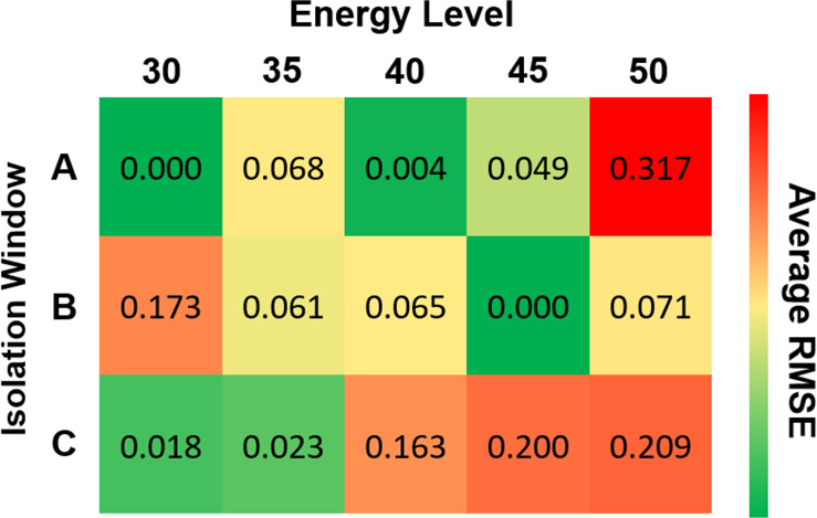
Sialic acids play important roles in many biological processes, including cell–cell communication and interaction, signaling, immune reactions, and carbohydrate–protein interactions.²⁶ The α2′–3′ to α2′–6′ ratio is important for multiple biological purposes and is a marker for early- and late-stage epithelial ovarian cancer.²⁷ Hence, we investigated the possibility of building a machine learning model to estimate the relative abundance of α2′–3′ using high MS level spectra. In this experiment, we utilized the MS⁵ spectra from the NIST standard data set and the MS⁴ spectra from the UGA-S data set, both of which share the same precursor ions. After removing outliers using 0.8 as the quality score threshold, we had 78 spectra from the UGA-S data set and 89 spectra from the NIST data set. We conducted four experiments. In the first one, we trained a model using the UGA-S data set and tested the model using the NIST data set. In the second one, we trained a model using the NIST data set and tested the model using the UGA-S data set. In the third one, we ran a 5-fold cross-validation using the UGA-S data set. In the last one, we ran a 5-fold cross-validation using the NIST data set. The results are summarized in Table 2 and show that the models, which are trained by the data of the A40, A45, B35, B40, B45, C35, and C45 protocols, are able to generalize well across data sets. Although the NIST data set does not contain mixtures of α2′–3′ and α2′–6′, the model trained by the NIST data set is able to generalize to the mixture samples in the UGA-S data set. The prediction uncertainty appears to be lower for purer samples (see details in Table S5), as the training data are glycans with pure α2′–3′ or α2′–6′ linkages.

Table 2. Linkage Ratio Inference Results (in RMSE) on MS^5,a.

	NIST → NIST	UGA-S → UGA-S	NIST → UGA-S	UGA-S → NIST
A30	0.007	0.027	0.104	0.084
A35	0.019	0.020	0.090	0.101
A40	0.066	0.015	0.094	0.050
A45	0.024	0.009	0.080	0.037
A50	0.166	0.013	0.087	0.184
B30	0.044	0.036	0.106	0.101
B35	0.084	0.025	0.086	0.118
B40	0.036	0.018	0.081	0.015
B45	0.080	0.014	0.082	0.001
B50	0.053	0.011	0.081	0.051
C30	0.049	0.040	0.109	0.090
C35	0.115	0.017	0.088	0.109
C40	0.003	0.010	0.086	0.008
C45	0.044	0.010	0.089	0.069
C50	0.036	0.010	0.084	0.030

^aThe row headers indicate the data collection configurations (see the Multilevel Mass Spectrometry section). The column headers indicate the training set (left) and the test set (right). NIST and UGA-S stand for the NIST and UGA-S data sets, respectively. When the training and test sets have the same name, the result is the average RMSE of the 5-fold cross-validation runs.

We also tested our approach on the UGA-R data set. The model was trained on the NIST data set and tested on the UGA-R data set (results in Table 3). The predictions of the relative α2′–3′ abundance vary as the spectra are of various quality indicated by their quality scores. Considering the spectra of high quality (quality score ≥ 0.8), the predicted relative α2′–3′ abundance range was from 0.4% to 37.3% in the positive control fetuin samples, from 0% to 2.2% in the positive control transferrin samples, and between 1.5% and 11.8% in the α2′–3′ neuraminidase fetuin samples.

Table 3. Linkage Regression Test on the UGA-R Data Set^a.

	+ control fetuin	+ control transferrin	α2′–3′ neuraminidase-treated fetuin
A30	26.6 (87.7)	0.0 (96.9)	28.4 (69.7)
A35	17.1 (80.7)	0.8 (95.1)	11.8 (88.3)
A40	37.2 (85.6)	0.8 (92.8)	19.7 (75.5)
A45	14.9 (90.5)	0.0 (97.0)	1.5 (93.0)
A50	37.3 (92.8)	0.0 (95.7)	55.5 (71.5)
B30	52.6 (48.2)	0.0 (96.6)	41.2 (76.6)
B35	0.4 (96.6)	0.0 (94.8)	77.4 (63.8)
B40	7.6 (94.2)	1.4 (94.9)	38.8 (72.1)
B45	29.7 (97.4)	0.0 (96.4)	28.3 (68.2)
B50	10.7 (88.3)	0.0 (94.2)	41.6 (59.6)
C30	28.2 (78.1)	0.0 (98.9)	80.7 (49.5)
C35	20.3 (90.6)	0.0 (98.1)	33.4 (64.0)
C40	6.3 (91.6)	2.2 (96.2)	6.4 (86.3)
C45	3.1 (96.4)	0.0 (97.0)	53.1 (52.6)
C50	10.3 (94.8)	0.0 (96.1)	6.7 (87.9)

^aThis table shows the estimated relative α2′–3′ abundance values and the corresponding sample quality scores (in parentheses) for positive control fetuin (+ control fetuin), positive control transferrin (+ control transferrin), and α2′–3′ neuraminidase-treated fetuin. Each row lists the results of a configuration in which the alphabetical character corresponds to the isolation window (A = 1, B = 2, C = 3, units of m/z), and the numerical characters correspond to the CID energy percentage (e.g., 30 = 30%, 45 = 45%).

Discriminant Power of Peaks in MS⁵ Basis Spectra

The MS⁵ basis spectra contain several peaks in addition to the conventional diagnostic signatures. There are eight peaks with relatively high abundance (≥0.1). Three of them are conventional diagnostic fragments (m/z = 103.08, 117.06, 131.07) reported in the literature,⁷ and the others are novel diagnostic fragments (m/z = 141.07, 143.08, 145.08, 173.11, and 175.13). We conducted ablation experiments to investigate the impact of these peaks on linkage regression. The linkage regressors were trained on the UGA-S data set and then applied to the NIST data set. We masked out the above peaks one-by-one and repeated the experiment for each data collection configuration. The results are presented in Supporting Information Table S4. Compared with the conventional fragments, some novel diagnostic fragments exerted comparable or even greater influence on estimating the relative α2′–3′ abundance. For example, the removal of conventional diagnostic signatures 103.08 or 131.07 led to an increase in RMSE in 9 and 4 out of 15 configurations, respectively. Removing the novel diagnostic fragment 175.13 led to large RMSE increases in 10 configurations. The exclusion of other novel diagnostic fragments also led to large RMSE increases in several configurations. Such observations indicate that the novel diagnostic fragments learned by NMF also provide essential information for linkage analysis.

Evaluate MSⁿ Configurations

We can evaluate an MS configuration by the average quality of the spectra collected under it. The quality of a spectrum is evaluated using eq 2, which hints at the reproducibility of the data. Figure 6 shows the average spectrum quality in the NIST and UGA-R data set. Configuration B45 (isolation window = 2, energy level = 45) achieves the best quality value, and configurations A45 and B35 are alternative good choices. Configurations B30, C30, and C50 are more likely to produce inconsistent signals. The quality values of individual MS levels are provided in Supporting Information Figure S2. Configurations A45, A50, B45, and B50 have the highest quality values at the MS² level. Configurations with energy level 35 produce high-quality spectra at the MS³ level. A similar pattern was observed at the MS⁴ level. At the MS⁵ level, configurations A30 and B45 produce spectra of higher quality.

Figure 6.

Average spectrum quality in the NIST and UGA-R data sets. The quality (the higher the better) of each configuration is the average quality of the MS^2/3/4/5 spectra in the NIST and UGA-R data sets.

Figure S3 in the Supporting Information compares the LOGO classification accuracies on the data collected under different configurations at individual MS^2/3/4 levels. We observed that configurations B35 and B40 produced the best classification results in MS², MS³, and MS⁴, meaning that they are the best configurations for the classification task. The relative α2′–3′ abundance estimation results (see Figure 7) suggest that the regression models trained on the data collected under A30, A40, and B45 can make precise estimations with RMSE less than 0.5%.

Figure 7.

Relative linkage abundance inference results (RMSE, stratified by the configuration) on the NIST data set. A model was trained on the spectra collected under each configuration in the UGA-S data set and was then tested on the NIST data set.

The classification models learned from any single configuration perform worse than the model presented in linkage classification on MS^2/3/4. The main cause for the performance drop is insufficient samples. The training data for one configuration contains 5 spectra. However, we achieve 90% classification accuracy and <0.5% regression error on the best configurations. The results suggest that with proper configuration, our classification pipeline and regression pipeline can make relatively accurate predictions with only one configuration.

Outlier Detection

We checked the distributions of the spectrum quality scores (Figure 8) and decided to choose the outlier threshold as 0.8. The spectra in the UGA-S data set are all of high quality (>0.9), as these samples are simpler than the samples used to collect the other two data sets. The 0.8 threshold detects 16 outliers in the NIST data set and 13 outliers in the UGA-R data set. Examples of outlier spectra at individual MSⁿ levels are shown in Supporting Information Figures S4–7.

Figure 8.

Outlier detection. The quality score distribution of the MS⁵ spectra in the NIST, UGA-S, and UGA-R data sets.

Scope of Application

Regarding glycans that contain both α2′–3′ and α2′–6′ linkages, our methodology is solely capable of predicting the ratio of these linkages in those glycans. However, it falls short in determining the specific arm upon which each linkage resides. We demonstrated our implementation of the proposed framework on differentiating sialic linkages in permethylated structures. Its application to native structures has yet to be validated. Although it is untested, it has the potential to work on other permethylated glycans, including milk oligosaccharides, glycolipids, and other O-linked glycans.

Conclusion

We propose a data-driven machine learning framework for distinguishing glycosidic linkages and estimating the ratio of linkages in a mixture using MSⁿ. The proof of principle was demonstrated by applying the framework to infer sialic acid linkages, more specifically α2′–3′ vs α2′–6′. We showed that the sialic acid isomers with α2′–3′ and α2′–6′ linkages can be differentiated by analyzing their MS⁴, MS³, or MS² spectra. We also showed that the MS⁵ spectra can be utilized to accurately estimate the ratio between α2′–3′ and α2′–6′ linkage in a mixture. Our approach includes an unsupervised learning component that uses NMF to learn the representations of the spectra. The learned representations are used to align spectra and remove outliers. Finally, we investigated data quality produced by different data collection protocol configurations and highlighted several configurations that are appropriate for differentiating α2′–3′ and α2′–6′ linkage using MSⁿ.

Our study demonstrates that machine learning holds promise in ameliorating the current challenges that sialic acid measurements pose to the scientific community. In the future, we plan to test our framework on more complex tasks, including other sialic acid linkages (e.g., α2′–8′) and monosaccharide isomers. We believe that the proposed framework is general and can be applied to analyze a variety of other glycosidic linkages. One of our ultimate goals is to elucidate the glycosidic linkages of polysaccharides using mass spectrometry, which is crucial in determining their biological properties.

Supporting Information Available

The Supporting Information is available free of charge at https://pubs.acs.org/doi/10.1021/jasms.3c00132.

• Experiment configurations used to collect the NIST, UGA-S, and UGA-R data sets; summary of the NIST, UGA-S, and UGA-R data sets; spectra outliers; influence of peaks in basis spectra; linkage regression uncertainty on the UGA-S data set; MS⁵ spectrum with fragmentation pathway; average spectrum quality at individual MS levels; average leave-one-glycan-out classification accuracy of different data collection configurations at individual MS levels; MS² outlier examples; MS³ outlier examples; MS⁴ outlier examples; MS⁵ outlier examples (PDF)

The authors declare no competing financial interest.

References

- Varki A. Colloquium paper: uniquely human evolution of sialic acid genetics and biology. Proc. Natl. Acad. Sci. U.S.A. 2010, 107 (Suppl 2), 8939–8946. 10.1073/pnas.0914634107. [DOI] [PMC free article] [PubMed] [Google Scholar]
- Ma X.; Li Y.; Kondo Y.; Shi H.; Han J.; Jiang Y.; Bai X.; Archer-Hartmann S. A.; Azadi P.; Ruan C.; Fu J.; Xia L. Slc35a1 deficiency causes thrombocytopenia due to impaired megakaryocytopoiesis and excessive platelet clearance in the liver. Haematologica 2021, 106 (3), 759–769. 10.3324/haematol.2019.225987. [DOI] [PMC free article] [PubMed] [Google Scholar]
- Shajahan A.; Supekar N. T.; Wu H.; Wands A. M.; Bhat G.; Kalimurthy A.; Matsubara M.; Ranzinger R.; Kohler J. J.; Azadi P. Mass Spectrometric Method for the Unambiguous Profiling of Cellular Dynamic Glycosylation. ACS Chem. Biol. 2020, 15 (10), 2692–2701. 10.1021/acschembio.0c00453. [DOI] [PMC free article] [PubMed] [Google Scholar]
- de Haan N.; Yang S.; Cipollo J.; Wuhrer M. Glycomics studies using sialic acid derivatization and mass spectrometry. Nature Reviews Chemistry 2020, 4, 229–242. 10.1038/s41570-020-0174-3. [DOI] [PubMed] [Google Scholar]
- Shajahan A.; Supekar N. T.; Chapla D.; Heiss C.; Moremen K. W.; Azadi P. Simplifying Glycan Profiling through a High-Throughput Micropermethylation Strategy. SLAS Technol. 2020, 25 (4), 367–379. 10.1177/2472630320912929. [DOI] [PMC free article] [PubMed] [Google Scholar]
- Black I.; Heiss C.; Carlson R. W.; Azadi P. Linkage Analysis of Oligosaccharides and Polysaccharides: A Tutorial. Methods Mol. Biol. 2021, 2271, 249–271. 10.1007/978-1-0716-1241-5_18. [DOI] [PubMed] [Google Scholar]
- Anthony R. M.; Nimmerjahn F.; Ashline D. J.; Reinhold V. N.; Paulson J. C.; Ravetch J. V. Recapitulation of IVIG Anti-Inflammatory Activity with a Recombinant IgG Fc. Science 2008, 320 (5874), 373–376. 10.1126/science.1154315. [DOI] [PMC free article] [PubMed] [Google Scholar]
- Shajahan A.; Supekar N.; Heiss C.; Azadi P. High-Throughput Automated Micro-permethylation for Glycan Structure Analysis. Anal. Chem. 2019, 91 (2), 1237–1240. 10.1021/acs.analchem.8b05146. [DOI] [PMC free article] [PubMed] [Google Scholar]
- Shajahan A.; Heiss C.; Ishihara M.; Azadi P. Glycomic and glycoproteomic analysis of glycoproteins-a tutorial. Anal Bioanal Chem. 2017, 409 (19), 4483–4505. 10.1007/s00216-017-0406-7. [DOI] [PMC free article] [PubMed] [Google Scholar]
- Sosicka P.; Ng B. G.; Pepi L. E.; Shajahan A.; Wong M.; Scott D. A.; Matsumoto K.; Xia Z. J.; Lebrilla C. B.; Haltiwanger R. S.; Azadi P.; Freeze H. H. Origin of cytoplasmic GDP-fucose determines its contribution to glycosylation reactions. J. Cell Biol. 2022, 221 (10), e202205038 10.1083/jcb.202205038. [DOI] [PMC free article] [PubMed] [Google Scholar]
- Anthony R. M.; Nimmerjahn F.; Ashline D. J.; Reinhold V. N.; Paulson J. C.; Ravetch J. V. Recapitulation of IVIG anti-inflammatory activity with a recombinant IgG Fc. Science 2008, 320 (5874), 373–376. 10.1126/science.1154315. [DOI] [PMC free article] [PubMed] [Google Scholar]
- Lee D. D.; Seung H. S. Learning the parts of objects by non-negative matrix factorization. Nature 1999, 401 (6755), 788–791. 10.1038/44565. [DOI] [PubMed] [Google Scholar]
- Adusumilli R.; Mallick P.. Data Conversion with ProteoWizard msConvert. In Methods in Molecular Biology; Springer: New York, 2017; pp 339–368. [DOI] [PubMed] [Google Scholar]
- Align peaks in signal to reference peaks - MATLAB msalign(r2023a); Mathworks, 2006; https://www.mathworks.com/help/bioinfo/ref/msalign.html (accessed 2023 July 23). [Google Scholar]
- Rapin J.; Souloumiac A.; Bobin J.; Larue A.; Junot C.; Ouethrani M.; Starck J.-L. Application of non-negative matrix factorization to LC/MS data. Signal Processing 2016, 123, 75–83. 10.1016/j.sigpro.2015.12.014. [DOI] [Google Scholar]
- Dubroca R.; Junor C.; Souloumiac A.. Weighted NMF for high-resolution mass spectrometry analysis. 2012 Proceedings of the 20th European Signal Processing Conference (EUSIPCO); IEEE, 2012; pp 1806–1810. [Google Scholar]
- Siy P. W.; Moffitt R. A.; Parry R. M.; Chen Y.; Liu Y.; Sullards M. C.; Merrill A. H.; Wang M. D.. Matrix factorization techniques for analysis of imaging mass spectrometry data. 2008 8th IEEE International Conference on BioInformatics and BioEngineering, Oct 2008; IEEE, 2008 [DOI] [PMC free article] [PubMed] [Google Scholar]
- Boutsidis C.; Gallopoulos E. SVD based initialization: A head start for nonnegative matrix factorization. Pattern Recognition 2008, 41 (4), 1350–1362. 10.1016/j.patcog.2007.09.010. [DOI] [Google Scholar]
- Bittremieux W.; Schmid R.; Huber F.; van der Hooft J. J. J.; Wang M.; Dorrestein P. C. Comparison of Cosine, Modified Cosine, and Neutral Loss Based Spectrum Alignment For Discovery of Structurally Related Molecules. J. Am. Soc. Mass Spectrom. 2022, 33 (9), 1733–1744. 10.1021/jasms.2c00153. [DOI] [PubMed] [Google Scholar]
- Eriksson J. O.; Sánchez Brotons A.; Rezeli M.; Suits F.; Markó-Varga G.; Horvatovich P. MSIWarp: A General Approach to Mass Alignment in Mass Spectrometry Imaging. Anal. Chem. 2020, 92 (24), 16138–16148. 10.1021/acs.analchem.0c03833. [DOI] [PMC free article] [PubMed] [Google Scholar]
- Griss J. Spectral library searching in proteomics. PROTEOMICS 2016, 16 (5), 729–740. 10.1002/pmic.201500296. [DOI] [PubMed] [Google Scholar]
- Stein S. Mass Spectral Reference Libraries: An Ever-Expanding Resource for Chemical Identification. Anal. Chem. 2012, 84 (17), 7274–7282. 10.1021/ac301205z. [DOI] [PubMed] [Google Scholar]
- Hearst M. A.; Dumais S. T.; Osuna E.; Platt J.; Scholkopf B. Support vector machines. IEEE Intelligent Systems and their Applications 1998, 13 (4), 18–28. 10.1109/5254.708428. [DOI] [Google Scholar]
- Guan W.; Zhou M.; Hampton C. Y.; Benigno B. B.; Walker L. D.; Gray A.; McDonald J. F.; Fernández F. M. Ovarian cancer detection from metabolomic liquid chromatography/mass spectrometry data by support vector machines. BMC Bioinformatics 2009, 10 (1), 259. 10.1186/1471-2105-10-259. [DOI] [PMC free article] [PubMed] [Google Scholar]
- Pedregosa F.; Varoquaux G.; Gramfort A.; Michel V.; Thirion B.; Grisel O.; Blondel M.; Prettenhofer P.; Weiss R.; Dubourg V.; Vanderplas J.; Passos A.; Cournapeau D.; Brucher M.; Perrot M.; Duchesnay E. Scikit-learn: Machine Learning in Python. J. Mach. Learn Res. 2011, 12, 2825–2830. [Google Scholar]
- Ghosh S.Sialic acid and biology of life: An introduction. Sialic Acids and Sialoglycoconjugates in the Biology of Life, Health and Disease; Elsevier, 2020; pp 1–61. [Google Scholar]
- Dedova T.; Braicu E. I.; Sehouli J.; Blanchard V. Sialic Acid Linkage Analysis Refines the Diagnosis of Ovarian Cancer. Frontiers in Oncology 2019, 9, 261. 10.3389/fonc.2019.00261. [DOI] [PMC free article] [PubMed] [Google Scholar]
Associated Data
This section collects any data citations, data availability statements, or supplementary materials included in this article.