Evaluating the Gray Level Co-Occurrence Matrix-Based Texture Features of Magnetic Resonance Images for Glioblastoma Multiform Patients’ Treatment Response Assessment

Abstract

Background:

Medical images of cancer patients are usually evaluated qualitatively by clinical specialists which makes the accuracy of the diagnosis subjective and related to the skills of clinicians. Quantitative methods based on the textural feature analysis may be useful to facilitate such evaluations. This study aimed to analyze the gray level co-occurrence matrix (GLCM)-based texture features extracted from T1-axial magnetic resonance (MR) images of glioblastoma multiform (GBM) patients to determine the distinctive features specific to treatment response or disease progression.

Methods:

20 GLCM-based texture features, in addition to mean, standard deviation, entropy, RMS, kurtosis, and skewness were extracted from step I MR images (obtained 72 h after surgery) and step II MR images (obtained three months later). Responded and not responded patients to treatment were classified manually based on the radiological evaluation of step II images. Extracted texture features from Step I and Step II images were analyzed to determine the distinctive features for each group of responsive or progressive diseases. MATLAB 2020 was applied to feature extraction. SPSS version 26 was used for the statistical analysis. P value < 0.05 was considered statistically significant.

Results:

Despite no statistically significant differences between Step I texture features for two considered groups, almost all step II extracted GLCM-based texture features in addition to entropy M and skewness were significantly different between responsive and progressive disease groups.

Conclusions:

GLCM-based texture features extracted from MR images of GBM patients can be used with automatic algorithms for the expeditious prediction or interpretation of response to the treatment quantitatively besides qualitative evaluations.

Introduction

A brain tumor, which can be benign or malignant, is an uncontrolled growth of cancerous cells in the brain. The structure of benign brain tumors is more homogenous without active cells, while malignant brain tumors are more heterogeneous in the structure and contain active cells.[1] Glioblastoma multiform (GBM) tumor is one of the most invasive and common types of primary malignant brain tumors.[2] The current standard treatment for GBM tumors includes surgery followed by chemotherapy and concomitant radiotherapy in addition to adjuvant chemotherapy with temozolomide (TMZ). TMZ is an oral alkylating agent used to treat GBM and astrocytoma tumors.[3]

For initial accurate detection of GBM tumors and also the evaluation of tumor response to the prescribed treatment, a contrast-weighted T1 magnetic resonance imaging (MRI) sequence is usually performed.[3] Contrast-weighted T1 MRI is the main applicable sequence for brain lesions imaging due to the ease of performing, as well as, accurate depiction of the margins of tumors.[4] Furthermore, evaluation of the tumor growth or destruction process and the treatment outcome is done mostly using MR imaging. An increase in contrast or an abnormal decrease in signal intensity in contrast-free imaging usually indicates disease progression.[3]

However, radiologists or clinical specialists usually evaluate such images qualitatively and visually. The diagnosis and extraction of the tumor area in such a way is a tedious and time-consuming task.[1,5] In addition, the accuracy of the diagnosis is subjective and depends mostly on the experience and skills of specialists.[1,5] Concerning these issues, quantitative assessment of MR images can be a good choice to improve the accuracy of detection and classification of brain tumors or to assess the response of the tumor to the delivered chemo or radiation therapy.[2,3]

Quantitative approaches commonly implement image texture analysis to detect brain abnormalities.[3] Texture analysis refers to a variety of mathematical techniques that can describe the gray surface patterns of an image or texture features.[6] Texture features provide a better description of the image and include information about the spatial distribution of changes in gray intensity levels.[7] Extraction of texture characteristics determines the homogeneity or similarity between different areas of an image. The extracted features contain information about an image that can be used as the input data for the automatic classification of images using the machine learning methods.[8]

The capability of quantitative techniques for brain tumor detection or to evaluate the treatment response and survival rate is shown in the literature. A study by Parekh et al.[9] proposed a multi-parametric radiomics feature extraction algorithm for the tissue analysis. The proposed algorithm distinguished grade IV brain tumors from Grade II with 93% sensitivity and 100% specificity. Furthermore, Kickingereder et al.[10] showed the feasibility of using an artificial neural network algorithm for quantitatively evaluation of brain MR images to assess the treatment response. Moreover, Ion-Margineanu et al.[11] proposed an automatic pipeline for processing multi-parametric MRI data of GBM patients treated with adjuvant therapy after surgery. Their proposed method was based on histogram and 3-D texture features, extracted from the regions of interest delineated manually and semi-manually. In another study, Ion-Margineanu et al.[12] used their previously proposed automatic algorithm to discriminate the treatment response or tumor progression quantitatively based on histogram and 3-D texture features for 29 GBM patients. Cheddad and Tanougast[13] studied gray level co-occurrence matrix (GLCM)-based texture features extracted from the MR images of 42 GBM patients and determined three textural features for predicting overall survival. Chen et al.[14] proposed a gradient-based classification framework for glioma tumor detection and grading based on structural MR images. They used the histogram of oriented gradients algorithm and the support vector machine (SVM) classifier. The proposed method showed an accuracy of 86.3% and a sensitivity of 89.4% in glioma detection. The glioma grading performance of the proposed algorithm revealed an accuracy of 76.3% and a sensitivity of 83.7%. They concluded that the gradient-based SVM classification algorithm could be a promising tool for automatically diagnosing and grading glioma tumors.

Concerning the mentioned introduction, this study aimed to determine the distinctive texture features between GBM patients who responded to the usual treatment regimes after surgery and patients with recurrence of the tumor. We focused on analyzing the textural features generated based on the GLCMs of T1-weighted axial MR images obtained 72 h and 3 months after surgery. The determined distinctive texture features or different combinations of these features can be used as training data for automatic machine learning or deep learning models. The automatic machine learning or deep learning algorithms trained by these features can be used to predict or classify the response to treatment or tumor relapse quantitatively, besides the qualitative evaluations which may be more subjective. The present study’s significance and novelty are using a relatively large sample size and considering the percentage differences of GLCM-based texture features at two follow-up steps after surgery to assess the response to treatment or tumor relapse.

Material and Methods

Studied patients and data collection

After approving the protocol by the Institutional Ethics Committee, clinical records of brain tumor patients under treatment in the radiation oncology ward were evaluated. GBM patients eligible to be included in the study were defined. Inclusion criteria comprised of diagnosed GBM tumor based on WHO measures,[15,16] the existence of the patient’s MR images (at least: initial diagnosis, 72 h after surgery, and three months after surgery) in the hospital PACS system, and the patient’s informed consent. Concerning the inclusion criteria, 96 GBM patients were included in the study. All these patients were receiving adjuvant therapy after surgery. All images were anonymized before use.

Applied magnetic resonance imaging system and evaluated magnetic resonance images

The MR images were acquired using a clinical 1.5 Tesla MRI system (Siemens, Germany), by a brain coil for transmission and an 8-channel head coil for signal reception. The imaging protocol consisted of conventional MRI (C-MRI). Obtained C-MRI sequences included axial T1, T2, and FLAIR, sagittal and coronal T2, in addition to the routine brain with gadolinium (axial T1⁺ contrast, sagittal T1⁺ contrast, and coronal T1⁺ contrast). A diffusion sequence was added for the patients with age ≥50 years.

From these C-MRI sequences, axial T1-weighted 3D gradient-echo scans after contrast administration obtained 72 h after surgery (called step I images) and three months after surgery (step II images) were used as high-resolution anatomical reference images for texture feature extraction. The used MR image acquisition parameters include Fast Field Echo (FFE), Repetition Time (TR)/ Time to Echo (TE): 0.019, flip angle: 90°, and acquisition voxel size: 1.1 mm × 0.9 mm × 5.5 mm.

Preprocessing of magnetic resonance images

For each patient, the image slice with the maximum cross-sectional area of the removed tumor vacancy from the first and second step images was selected by a radiation oncologist with enough work experience. These DICOM images were imported into the scientific software package MATLAB (R2020, The Math Works, Inc., Natick, MA, USA) and preprocessed using an in-house prepared code. Preprocessing comprised of registration of the selected step I and step II T1axial MR slices for each patient, segmenting the tumoral area, and grayscale discretizing. Affine model based on similarity initial condition algorithm was used for registration. Using the co-registered images, the dimensions of the mask needed to segment the same tumoral area (including surgery cavity and edema surrounding area or relapsed enhanced parts of tumor) from the two images of each patient were determined. Using this mask, the same areas from both selected slices of first and second follow-up MR images were segmented. Discretization of grayscale intensities to 256 gray levels was carried out for these segmented images before texture feature extraction.

Feature extraction

Gray level co-occurrence coefficients (GLCMs) have been used in this study. The GLCM coefficients prepare a second-order approach for generating the texture features of images. These coefficients show the conditional joint probabilities of all pairs with combinations of gray levels in the spatial window of interest given two parameters: Interpixel distance (δ) and orientation (θ). The probability measure is stated as:

Where Cij (the co-occurrence probability between gray levels i and j) is determined as:

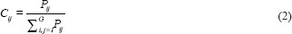
where Pij indicates the number of occurrences of gray levels i and j within the given window, given a certain (δ, θ) pair; and G is the quantized number of gray levels. The sum in the denominator illustrates the total number of gray level pairs (i, j) within the window.[4]

Using a prepared MATLAB code and graycomatrix syntax, GLCM coefficients were extracted from preprocessed segmented tumoral areas of Step I and II images for all included patients in four different directions (0°, 45°, 90°, and 135°) with an interpixel distance of 1. Texture (Haralick[17]) features [mentioned in Table S1 of Supplementary Files] were generated based on extracted GLCMs. Moreover, six statistics of mean, standard deviation, RMS, entropy, skewness, and kurtosis were calculated directly for extracted GLCMs. Therefore, four vectors of texture features were configured each consisting of 26 extracted statistics. These four vectors were summed and averaged to have a unique vector of texture features. It should be mentioned that the direct calculated entropy feature is shown as entropy M in the whole text to be different of entropy feature generated using graycomatrix syntax.

Table S1.

Gray level co-occurrence matrix-based texture features

Statistics	Reference	Statistics	Reference
Autocorrelation =	[2]	MP=Maximum. P (i, j) for all (i, j)	[2]
Contrast =	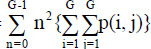[3,18]	Variance =	[3]
	[3,18]	Sum average or mean =	[1,19]
Cluster prominence =	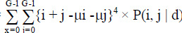[3]		[19]
	[2,3]		[19]
Dissimilarity =	[6]		[19]
Energy =	[18]		[19]
Entropy =	[1]	Information measures of correlation 1 =	[8,20]
	[8]	Information measures of correlation 2 =	[8]
	[19]	Homogeneity =	[8]
	[6]		[6]

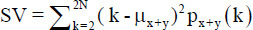
MCC was not calculated due to computational instability. IDM was also not calculated due to its similarity to the homogeneity feature. Correlation and homogeneity were calculated based on the MATLAB method (graycomatrix syntax) and the formula presented by Soh and Tsatsoulis[2] which gave the same results. MP – Maximum probability; CS–Cluster shade; IDM – Inverse difference moment; IDN – Inverse difference normalized; CC – Correlation coefficient; DE – Difference entropy; DV – Difference variance; SE – Sum entropy; SV – Sum variance; MCC – Maximal CC; ID – Inverse Difference

Manually classification of patients

The included patients were classified manually by the radiation oncologist, and each patient was assigned to one of two considered clinical groups including responded and not responded to treatment (responsive and progressive disease) groups.

Manually classification of patients and assigning them to each group of responsive or progressive disease was done based on the radiologic evaluation of follow-up C-MRI sequences using available guidelines to assess the treatment response of GBM patients (the MacDonald[21] and RANO[22] Criteria). A summary of these criteria is presented in Table S2 of Supplementary Files. Using these measures and the method of Ion-Margineanu et al. 2017,[12] the patients whose tumor vacancy in the step I images had been filled in the follow-up images, and all measurable or nonmeasurable lesions had disappeared were assigned to the responsive disease group. Patients with progressive disease were determined as patients with an increase of ≥25% in the sum of the products of the perpendicular diameter of enhancing lesions compared to the smallest tumor measurement obtained either at baseline or best response. Concerning the mentioned measures, 49 patients were labeled as responded and 47 patients were labeled as nonresponded.

Table S2.

Summary of Macdonald and response assessment in neuro-oncology measures to evaluate the glioblastoma multiform patient’s treatment response

	Macdonald	RANO
Response*	The disappearance of all enhancing measurable and nonmeasurable lesions (sustained for≥4 weeks) No new lesions Clinical stability or improvement	Disappearance of all enhancing measurable and nonmeasurable lesions (sustained for≥4 weeks) Stable or improved nonenhancing lesions based on T2/FLAIR MR sequences No new lesions Clinically stable or improved
Progression	25% or more increase in enhancing lesions Clinical deterioration	Significant increase in nonenhancing lesions (T2/FLAIR) those not caused by comorbid events Any new lesion Clear clinical deterioration (not attributable to other causes from the tumor or changes in corticosteroid dose) A clear progression of nonmeasurable lesions

*The mentioned conditions are for a complete response. There are also, some conditions to detect partial response or stable disease situations based on Macdonald and RANO criteria.[21,22,23,24] MR – Magnetic resonance; RANO – Response assessment in neuro-oncology; T2/FLAIR – Weighted-Fluid-Attenuated-Inversion Recovery

Analysis

The calculated step I GLCM-based texture features and direct statistics of MR images for all included patients were compared to step II features of each responded and not responded group. Also, step II extracted textural features were compared between two groups of responded and nonresponded patients to define the distinctive features between the two considered groups. Moreover, percentage differences of extracted features between the two follow-up steps for both responded and not responded patients were calculated and evaluated. The percentage differences (PD) were calculated using Eq. 3.

Statistical analysis was conducted using the SPSS software version 26 (IBM Corp. Released 2019. IBM SPSS Statistics for Windows, Version 26.0. Armonk, NY: IBM Corp). The independent sample t-test was used to compare the means of extracted features between responded and not responded groups and follow-up steps. P <0.05 was considered statistically significant. Figure 1 shows the flowchart of the present study.

Figure 1.

Flowchart of the study

Results

Demographic characteristics of 96 evaluated GBM patients and their treatment method are revealed in Table 1. C-MRI sequences including T1 axial with contrast, T2, T2 FLAIR, ADC, and diffusion sequences for a responded and a not responded patient which are obtained 72 h after surgery (step I) and three months later (step II) are depicted in Figures 2 and 3, respectively. Figure 4 represents step I and II images of a sample patient registered using the affine model to determine the tumoral area and mask dimension for segmenting the same areas from two follow-up MR images.

Table 1.

Demographic characteristics of 96 glioblastoma multiform patients involved in the study and their treatment method

Characteristic	Frequency (%) of patients
Mean patients age (years)	39.80±11.04
Age range (years)	6–71
Gender
Male	66 (68.8%)
Female	30 (31.3%)
Tumor pathology
GBM	100%
Treatment method
Surgery + radiotherapy + chemotherapy TMZ	96 (100%)

GBM – Glioblastoma multiform; TMZ – Temozolomide

Figure 2.

C-MRI sequences of an evaluated patient obtained 72 h after surgery (step I) and three months later (step II) show response to the treatment. C-MRI: Conventional-magnetic resonance imaging

Figure 3.

C-MRI sequences of an evaluated patient obtained 72 h after surgery (step I) and three months later (step II) illustrate the disease progression and tumor relapse after surgery. C-MRI: Conventional-magnetic resonance imaging

Figure 4.

A sample of registered images to define the tumoral area and crop the same area of both step images

The mean ± standard deviations of 26 generated GLCM-based texture features and statistics extracted from a segmented area of reference images of all included patients (step I features), and second follow-up images of responsive and progressive disease groups (step II features) in addition to the P values to compare means are reported in Table 2. Table 3 shows the P values to compare the step II texture features between clinically responsive and progressive disease groups. Furthermore, Figure 5 shows the percentage differences of all extracted features for each group of responsive and progressive diseases.

Table 2.

Average of gray level co-occurrence matrix-based texture features extracted from step I (reference) images of all included patients (96) compared to the average of these features extracted from step II (follow-up) images of responded and not responded patients (step I: 72 h after surgery, step II: 3 months after surgery)

Textural feature	Mean±SD		P	Not responded patients (step II) n=47	P
	All included patients (step I) n=96	Responded patients (step II) n=49
Autocorrelation	7.26±2.40	6.45±2.20	0.045*	9.08±2.89	0.000*
Contrast	0.19±0.10	0.14±0.05	0.002*	0.21±0.08	0.120
Correlation	0.80±0.07	0.79±0.06	0.630	0.83±0.06	0.019*
Cluster prominence	16.95±24.59	8.43±10.73	0.022*	30.96±28.60	0.003*
Cluster shade	0.59±2.37	−0.21±1.93	0.031*	1.84±3.43	0.012*
Dissimilarity	0.17±0.07	0.13±0.04	0.001*	0.19±0.06	0.053
Energy	0.39±0.14	0.45±0.14	0.006*	0.33±0.13	0.026*
Entropy	1.43±0.39	1.20±0.29	0.001*	1.64±0.39	0.003*
Homogeneity	0.92±0.03	0.94+0.02	0.001*	0.91±0.03	0.041*
Maximum probability	0.56±0.14	0.61±0.14	0.031*	0.51±0.14	0.042*
Sum of squares: Variance	7.36±2.39	6.52±2.20	0.040*	9.193±2.90	0.000*
Sum average	5.16±0.89	4.88±0.92	0.086	5.75±0.93	0.001*
Sum variance	17.51±6.66	16.39±6.67	0.342	21.53±7.30	0.002*
Sum entropy	1.29±0.33	1.10±0.26	0.000*	1.48±0.34	0.003*
Difference variance	0.19±0.10	0.14±0.05	0.002*	0.21±0.08	0.120
Difference entropy	0.45±0.12	0.38±0.09	0.001*	0.49±0.11	0.027*
Information measure of correlation 1	−0.49±0.08	−0.50±0.08	0.302	−0.50±0.07	0.421
Information measure of correlation 2	0.76±0.08	0.73±0.08	0.059	0.80±0.07	0.005*
Inverse difference (ID)	0.999±0.0003	0.999±0.0002	0.001*	0.999±0.00	0.053
IDN	1.00±0.00	1.00±0.00	0.002*	1.00±0.00	0.120
Mean	0.10±0.07	0.10±0.08	0.950	0.10±0.06	0.830
SD	15.65±12.70	16.57±13.85	0.696	14.27±10.90	0.505
Entropy M	0.004±0.001	0.003±0.001	0.007*	0.004±0.001	0.018*
RMS	15.65±12.70	16.577±13.85	0.696	14.27±10.90	0.505
Kurtosis	47,192.38±11,582.17	49,682.10±12,453.64	0.247	44,657.40±12,641.48	0.235
Skewness	209.16±29.11	216.30±30.22	0.176	202.52±31.65	0.230

*Statistically significant differences. P values belong to comparing step 1 features of all included patients with step II of responded and not responded ones. IDN – Inverse difference normalized; SD – Standard deviation; ID – Inverse difference; RMS – Root mean square

Table 3.

Average of step II (second follow-up) gray level co-occurrence matrix-based texture features for responded patients compared to not responded ones (second follow-up: 3 months after surgery)

GLCM feature	Mean±SD		P
	Responded patients (step II) n=49	Not responded patients (step II) n=47
Autocorrelation	6.45±2.20	9.08±2.89	0.000*
Contrast	0.14±0.05	0.21±0.08	0.000*
Correlation	0.79±0.06	0.83±0.06	0.012*
Cluster prominence	8.43±10.73	30.96±28.60	0.000*
Cluster shade	−0.21±1.93	1.84±3.43	0.000*
Dissimilarity	0.13±0.04	0.19±0.06	0.000*
Energy	0.45±0.14	0.33±0.13	0.000*
Entropy	1.20±0.29	1.64±0.39	0.000*
Homogeneity	0.94±0.02	0.91±0.03	0.000*
Maximum probability	0.61±0.14	0.51±0.14	0.000*
Sum of squares: Variance	6.52±2.20	9.193±2.90	0.000*
Sum average	4.88±0.92	5.75±0.93	0.000*
Sum variance	16.39±6.67	21.53±7.30	0.001*
Sum entropy	1.10±0.26	1.48±0.34	0.000*
Difference variance	0.14±0.05	0.21±0.08	0.000*
Difference entropy	0.38±0.09	0.49±0.11	0.000*
Information measure of correlation 1	−0.50±0.08	-0.50±0.07	0.823
Information measure of correlation 2	0.73±0.08	0.80±0.07	0.000*
Inverse difference (ID)	0.9995±0.0002	0.9992±0.0002	0.000*
IDN	1.00±0.00	1.00±0.00	0.000*
Mean	0.10±0.08	0.10±0.06	0.816
SD	16.57±13.85	14.27±10.90	0.367
Entropy M	0.00±0.00	0.00±0.00	0.000*
RMS	16.577±13.85	14.27±10.90	0.367
Kurtosis	49,682.10±12,453.64	44,657.40±12,641.48	0.053
Skewness	216.30±30.22	202.52±31.65	0.032*

*Shows the statistical significance differences. GLCM – Gray level co-occurrence matrix; IDN – Inverse difference normalized; SD – Standard deviation; RMS – Root mean square; ID – Inverse difference

Figure 5.

The mean percentage differences of extracted GLCM-based texture features and direct statistics between reference and follow-up images (step I and II, T1 axial + GD sequences) for responded and not responded patients. GLCM – Gray level co-occurrence matrix

Discussion

Reliable imaging assessment can be challenging for GBMs due to heterogeneous angiogenesis, cellular proliferation, cellular invasion, and apoptosis, which can cause different grades of necrosis, solid-enhancing tumors, peritumoral tissue, and peritumoral edema. Therefore, the texture feature analysis techniques may be well suited to solving such image-based problems of the accurate and expeditious interpretation of large-quantity and complex data.[22] Radiomics is a high throughput process of image feature extraction that uses texture features to predict response and patient survival and to gather biological information about the disease.[25] The present study focused on analyzing GLCM-based texture features extracted from two postsurgery MR images of GBM patients. To determine distinctive texture features specific to responded and not responded patients to delivered treatment, MR images of 96 GBM patients were evaluated. A MATLAB code was developed to extract GLCM-based texture features from C-MRI T1-axial sequences (step I: obtained 72 h after surgery and step II: three months later). Our work consisted in analyzing 20 texture features derived from GLCMs generated for one-pixel displacement distance (d = 1) in four different directions as well as 6 direct statistics calculated for extracted GLCMs. GLCMs allow the characterization of pattern repetitions.[26]

GLCM-based textural features were calculated for step I images of all included patients. Then the patients were manually divided into two clinical groups of responsive and progressive disease according to the radiologic evaluation of follow-up C-MR images and based on RANO[22] and Macdonald[21] measures. Concerning the mentioned measures, 49 patients were classified as responding to the delivered treatment while 47 patients were placed in the not responded or progressive disease group. The same features were obtained from step II (follow-up) images of patients in each group and compared.

Based on the results, both groups were homogenous and no statistically significant differences were seen between mean ages, genders, or extracted step I texture features of two considered patient groups.

According to findings, autocorrelation decreased for responded patients while increased for not responded ones in step II images compared to step I. The differences in autocorrelation features between two steps for each group and between two groups of responsive and progressive disease were statistically significant. Since the autocorrelation of GLCMs measures the magnitude of the fineness and coarseness of textural patterns,[27,28] this result is expected and in line with the findings of Karthikeyan and Rengarajan[29] who obtained the higher values of autocorrelation for abnormal images.

According to th findings, the contrast feature as a measure of local variations of gray levels or intensity variations between the reference pixel and its neighbor[30,31] reduced statistically significant for responded patients while increased for not responded ones. The step II contrast features showed statistically significant differences between responded and not responded patients. Large contrast reflects large intensity differences in GLCMs.[32] Hence, local variations will decrease along with patient well-being and filling of the surgery cavity with normal brain tissue. This finding is consistent with the results of other studies.[9,29,33]

Furthermore, correlation as a measure of gray level linear dependency between neighboring pixels[3,32,33] was assessed. Despite a slight decrease in correlation features for responded patients, a statistically significant increase in correlation features was observed for not responded patients. Also, the correlation feature showed statistically significant differences between step II MR images of responded and not responded patients. This is while Karthikeyan and Rengarajan[29] observed a slightly higher correlation for normal tissues compared to abnormal tissues for glaucoma diagnosis. Furthermore, Yang et al.[33] reported higher values of correlation features for normal parotid tissue ultrasound images compared to parotid tissue exposed to radiation for head-and-neck cancer patients. Moreover, the results of Parkhe et al.[9] revealed a higher correlation extracted from MR images for Grade II glioma compared to grade IV.

Cluster shade is a measure of the skewness of the matrix, which is believed to gauge the perceptual concepts of uniformity. Cluster prominence is a measure of asymmetry.[3] Cluster prominence and cluster shade decreased for responded patients to treatment while these features raised for not responded groups. The differences in these features between the two steps and also two groups of responded and not responded patients were statistically significant. These findings agreed with the results of Karthikeyan and Rengarajan,[29] who observed the higher values of the cluster shade and cluster prominence features for abnormal tissues. When the cluster prominence value is high, the image is less symmetric. In addition, when the cluster prominence value is low, there is a peak in the GLCM matrix around the mean values.[3]

Dissimilarity as a measure of distance between pairs of objects (pixels) in the region of interest[34] was calculated. This feature measures the gray level mean difference in the distribution of the image. A larger value implies a greater disparity in intensity values among neighboring pixels.[34] Dissimilarity was reduced statistically significant for responded patients to treatment while increased in step II images of not responded patients which shows the higher inhomogeneity and variations in pixel values of these images.

Energy or angular second moment as a measure of uniformity provides the sum of squared elements and ranges from 0 to 1 for an image.[35] This feature increased for responded patients to treatment while reduced for not responded ones. The differences in energy features between the two considered steps and groups were statistically significant. This result is consistent with other researchers’ findings.[28,29,32] The reduction of energy illustrates lower uniformity of not responded patients’ images and the GLCMs of the less homogeneous images will have a large number of small entries.[35]

In addition, entropy as a measure of randomness of a gray level distribution[35] decreased for responded patients while raised for not responded ones. Again, the entropy differences between the two considered steps and groups were statistically significant. This finding is in line with other studies.[9,29] So that, the study by Marwah et al. 2015[36] reported energy increment and entropy decrement with responding to treatment as the tissue becomes smoother and more homogenous after treatment. Entropy is large when the image is not texturally uniform and many GLCM elements have very small values. As entropy measures the complexity of an image, complex textures tend to have higher entropy. Entropy is strongly but inversely correlated to the energy.[35]

The homogeneity feature differences between the two steps and step II images of two considered groups were statistically significant, with higher values for responded patients. This finding coincides with other studies.[9,13,28]

Furthermore, the maximum probability feature which measures the maximum likelihood of producing the pixels of interest,[34] increased for responded patients while decreased for the progressive disease group. The variations between the two steps and step II images of the two considered groups were statistically significant. This finding coincides with the results of Karthikeyan and Rengarajan.[29]

The sum of squares or variance feature as a measure of inhomogeneity or dispersion reduced significantly with responding to the treatment which agrees with the literature.[36] The differences in step II extracted variances were statistically significant with a higher value for not responded patients. Since the variance feature indicates how spread out the distribution of gray levels is, this feature is expected to be higher for images with more spread out gray levels.[36]

The sum average feature measures the mean of the gray levels sum distribution of an image.[34] This feature is calculated by adding all the pixel values divided by the total number of pixels in an image.[1] Furthermore, sum variance and difference variance are the combinations of all variances. The sum average, sum variance, and difference variance features decreased along with patient well-being while showing the reverse trend for not responded patients. The differences in these features were statistically significant between responsive and progressive disease groups. These findings are consistent with the results of Marwah et al.[36] who showed a decrease in variance feature with the patient well-being and increasing image homogeneity. The sum entropy feature which is related to the sum variance feature was statistically different between two follow-up steps and two considered groups of patients, with higher values for not responded ones. This finding is also reported by the study of Karthikeyan and Rengarajan.[29] The same trend was observed for the difference entropy feature.

The informational measure of correlation 1 is a function of the joint probability density distribution P (x, y) of the two variables x and y. In addition, the measure of dependency between two random variables (x and y) as a function of the amount of information in one random variable compared to the other, is called the informational coefficient of correlation 2.[8] According to the findings, the information measure of correlation 2 feature showed statistically significant differences between step II images of responsive and progressive disease groups with higher values for the latter group, which is also reported by Parkh et al.[9] This is while information measure of correlation 1 showed no significant differences between two steps or two groups.

Inverse difference and inverse difference normalized showed statistically significant differences between step II images of responded and not responded patients. Our results are in accordance with the study of Chaddad and Tanougast[13] who reported the statistically significant differences in difference entropy, information measure of correlation, and inverse difference texture features derived from active tumor parts for responsive or progressive disease groups. They concluded that these features can be used for the prediction of overall survival for GBM patients.

Among six direct calculated statistics, only entropy M and skewness showed statistical differences between Step II images of two considered groups, with higher entropy for not responded group and higher skewness for responded patients.

Our results are in accordance with Mehrabian et al.[37] who evaluated the treatment response of two patients with brain metastases and observed more heterogeneous images for the patient with recurrent tumors after surgery. findings of the Fujima et al.[38] showed higher contrast and lower homogeneity for squamous cell carcinoma patients compared to malignant lymphoma patients. Furthermore, findings of other studies[1,27] revealed significantly higher entropy, skewness, kurtosis, contrast, and informational measure of correlation1 for high-grade gliomas compared to low-grade tumors and lower values of correlation and homogeneity for low-grade gliomas patients.

Moreover, Patel et al.[39] reported higher kurtosis, entropy, contrast, and lower correlation values for true progression of brain tumors compared to pseudo-progression on T2-weighted MR images. Furthermore, Assefa et al.[40] reported that the sum average and variance texture features offer the best results in discriminating brain tissue from tumors in both the T1-weighted and T2-FLAIR image sets. They have also stated the performance of energy and maximum probability features for regional texture identification.

Based on the results, the percentage differences of most of the GLCM-based texture features and direct statistics calculated using Eq. 3, varied significantly between responsive and progressive disease groups of patients. As shown in Figure 5, among studied features, cluster prominence and cluster shade showed the highest percentage differences between the two step images for both responsive and progressive disease groups. Also, almost all GLCM-based texture features and direct statistics showed the reverse trend of variations between the two steps images for responded and not responded patients to treatment. In summary, step II features include autocorrelation, contrast, correlation, cluster prominence, cluster shade, dissimilarity, entropy, variance, sum average, sum variance, sum entropy, difference variance, difference entropy, information measure of correlation 2, mean, and entropy M decreased compared to step I features for responded patients while increased for patients whose tumor relapsed. Furthermore, energy, homogeneity, maximum probability, standard deviation, RMS, kurtosis, and skewness features increased for responded patients in step II images compared to step I ones. The reverse trend was observed for patients with tumor relapse in follow-up images. Only exception was information measure of correlation 1, which showed same percentage of variations for both considered groups of patients. Although the statistically significant differences between inverse difference and inverse difference normalized features between step II images of responsive and progressive disease groups, the percentages differences of these features between step I and II for each group was very low (close to zero) [Figure 5].

It should be pointed out that, additional perfusion sequences or MRS technique may be required for accurate diagnosis and assessment of the tumor response to a delivered treatment. Due to the limitations of our MRI system and the lack of such facilities in our clinic, only C-MRI sequences were used in our study which is a limitation of our work. In addition, since performing any further examinations for the patients was forbidden because of the ethics and clinical situation of the patients, we only used the available MR images which belonged to two standard follow-up steps. For future works, to improve the accuracy of assessing the response to treatment, if the clinical situation of included patients and ethics committee permit, more imaging steps with smaller time intervals is proposed to have more time points and to improve the prediction efficiency of the proposed method. This may result in estimating the response to treatment more accurately, the differentiation between high- and low-grade GBMs, bleeding and recurrence of the tumor, and the necrotic areas. Another limitation of our study is selecting slices with the maximum tumoral area manually by clinical expert. This process may be associated with some inevitable errors. It is recommended to prepare a code or use any available software to do this procedure automatically for future studies.

Conclusions

20 GLCM-based texture features and six direct statistics as a promising and efficient technique for image analysis[28] have been extracted and evaluated to determine quantitative measures applicable for evaluating the GBM patients’ response to treatment besides the subjective analysis of MRI images by radiologists.

Despite no significant differences between step I extracted texture features for two considered groups, almost all step II extracted GLCM-based texture features in addition to entropy M and skewness statistics showed statistically significant differences between the two considered groups of responsive and progressive disease. The step II GLCM-based texture features with statistically significant differences between manual classified responsive and progressive disease groups include contrast, correlation, cluster prominence, cluster shade, dissimilarity, entropy, energy, homogeneity, maximum probability, variance, sum average, sum variance, sum entropy, difference variance, difference entropy, information measure of correlation 2, inverse difference, and inverse difference normalized features. Almost all GLCM-based texture features and direct statistics showed the reverse trend of variations between the two steps images for responded and not responded patients to treatment.

It can be concluded that GLCM-based texture features extracted from MR images of GBM patients can be used as distinctive features between two groups of responsive and progressive diseases. As almost all GLCM-based texture features extracted from follow-up MR images of GBM patients are significantly different between responsive and progressive disease groups of patients, these features and their percentage differences between the two steps of follow up can be used as training data for automatic classification algorithms for expeditious prediction or interpretation of the response to treatment quantitatively besides qualitative evaluations.

Financial support and sponsorship

This study is a part of the MSc thesis of Sanaz Alibabaei which is financially supported by Jundishapur Ahvaz University of Medical Sciences (Grant No.CRC-0001). The protocol was approved by the ethics committee of Ahvaz Jundishapur University of Medical Sciences (Ref. No.: CRC-0001, Ethics code: IR.AJUMS.MEDICINE.REC.1399.051). Patients’ informed consent was obtained, and all images were anonymized before use.

Conflicts of interest

There are no conflicts of interest.

References

- 1.Bahadure NB, Ray AK, Thethi HP. Image analysis for MRI based brain tumor detection and feature extraction using biologically inspired BWT and SVM. Int J Biomed Imaging. 2017;2017:1–12. doi: 10.1155/2017/9749108. [DOI] [PMC free article] [PubMed] [Google Scholar]
- 2.Soh LK, Tsatsoulis C. Texture analysis of SAR sea ice imagery using gray level co-occurrence matrices. IEEE Trans Geosci Remote Sens. 1999;37:780–95. [Google Scholar]
- 3.Albregtsen F. Statistical texture measures computed from gray level co-occurrence matrices. Image Process Lab Dep Inform Univ Oslo. 2008;5:1–14. [Google Scholar]
- 4.Clausi DA. An analysis of co-occurrence texture statistics as a function of grey level quantization. Can J Remote Sens. 2002;28:45–62. [Google Scholar]
- 5.Xu Y, Wang Y, Yuan J, Cheng Q, Wang X, Carson PL. Medical breast ultrasound image segmentation by machine learning. Ultrasonics. 2019;91:1–9. doi: 10.1016/j.ultras.2018.07.006. [DOI] [PubMed] [Google Scholar]
- 6.Dinesh DP. Texture Image Classification Using Hybridization of GLCM and GLWM Features. International Journal of Scientific and Technology Research. 2020;9(04):3216–19. [Google Scholar]
- 7.Armi L, Fekri-Ershad S. Texture image analysis and texture classification methods-A review. arXiv. 2019;2:1–29. [Google Scholar]
- 8.Brynolfsson P, Nilsson D, Torheim T, Asklund T, Karlsson CT, Trygg J, et al. Haralick texture features from apparent diffusion coefficient (ADC) MRI images depend on imaging and pre-processing parameters. Sci Rep. 2017;7:4041. doi: 10.1038/s41598-017-04151-4. [DOI] [PMC free article] [PubMed] [Google Scholar]
- 9.Parekh VS, Laterra J, Bettegowda C, Bocchieri AE, Pillai JJ, Jacobs MA. Multiparametric deep learning and radiomics for tumor grading and treatment response assessment of brain cancer:Preliminary results. 2019:1–6. arXiv preprint arXiv: 1906.04049. [Google Scholar]
- 10.Kickingereder P, Isensee F, Tursunova I, Petersen J, Neuberger U, Bonekamp D, et al. Automated quantitative tumour response assessment of MRI in neuro-oncology with artificial neural networks:A multicentre, retrospective study. Lancet Oncol. 2019;20:728–40. doi: 10.1016/S1470-2045(19)30098-1. [DOI] [PubMed] [Google Scholar]
- 11.Ion-Margineanu A, Van Cauter S, Sima DM, Maes F, Van Gool SW, Sunaert S, et al. Tumour relapse prediction using multiparametric MR data recorded during follow-up of GBM patients. Biomed Res Int. 2015;2015:842923. doi: 10.1155/2015/842923. [DOI] [PMC free article] [PubMed] [Google Scholar]
- 12.Ion-Mărgineanu A, Van Cauter S, Sima DM, Maes F, Sunaert S, Himmelreich U, et al. Classifying glioblastoma multiforme follow-up progressive versus responsive forms using multi-parametric MRI features. Front Neurosci. 2016;10:615. doi: 10.3389/fnins.2016.00615. [DOI] [PMC free article] [PubMed] [Google Scholar]
- 13.Chaddad A, Tanougast C. Extracted magnetic resonance texture features discriminate between phenotypes and are associated with overall survival in glioblastoma multiforme patients. Med Biol Eng Comput. 2016;54:1707–18. doi: 10.1007/s11517-016-1461-5. [DOI] [PubMed] [Google Scholar]
- 14.Chen T, Xiao F, Yu Z, Yuan M, Xu H, Lu L. Detection and grading of gliomas using a novel two-phase machine learning method based on MRI images. Front Neurosci. 2021;15:650629. doi: 10.3389/fnins.2021.650629. [DOI] [PMC free article] [PubMed] [Google Scholar]
- 15.Dumba M, Fry A, Shelton J, Booth TC, Jones B, Shuaib H, et al. Imaging in patients with glioblastoma:A national cohort study. Neurooncol Pract. 2022;9:487–95. doi: 10.1093/nop/npac048. [DOI] [PMC free article] [PubMed] [Google Scholar]
- 16.Sanghvi D. Post-treatment imaging of high-grade gliomas. Indian J Radiol Imaging. 2015;25:102–8. doi: 10.4103/0971-3026.155829. [DOI] [PMC free article] [PubMed] [Google Scholar]
- 17.Haralick RM. Statistical and structural approaches to texture. Proc IEEE. 1979;67:786–804. [Google Scholar]
- 18.Kumar P, Vijay Kumar B. Brain tumor MRI segmentation and classification using ensemble classifier. Int J Recent Technol Eng (IJRTE) 2019;8:244–52. [Google Scholar]
- 19.Selvaraj D, Dhanasekaran RJ. A review on current MRI brain tissue segmentation feature extraction and classification techniques. International Journal of Electronics,Communication &Instrumentation EngineeringResearch and Development. 2013;3:21–30. [Google Scholar]
- 20.Linfoot EH. An informational measure of correlation. Inf Control. 1957;1:85–9. [Google Scholar]
- 21.Chinot OL, Macdonald DR, Abrey LE, Zahlmann G, Kerloëguen Y, Cloughesy TF. Response assessment criteria for glioblastoma:Practical adaptation and implementation in clinical trials of antiangiogenic therapy. Curr Neurol Neurosci Rep. 2013;13:347. doi: 10.1007/s11910-013-0347-2. [DOI] [PMC free article] [PubMed] [Google Scholar]
- 22.Chukwueke UN, Wen PY. Use of the response assessment in neuro-oncology (RANO) criteria in clinical trials and clinical practice. CNS Oncol. 2019;8 doi: 10.2217/cns-2018-0007. CNS28. [DOI] [PMC free article] [PubMed] [Google Scholar]
- 23.Sharma M, Juthani RG, Vogelbaum MA. Updated response assessment criteria for high-grade glioma:Beyond the MacDonald criteria. Chin Clin Oncol. 2017;6:37. doi: 10.21037/cco.2017.06.26. [DOI] [PubMed] [Google Scholar]
- 24.Wen PY, Macdonald DR, Reardon DA, Cloughesy TF, Sorensen AG, Galanis E, et al. Updated response assessment criteria for high-grade gliomas:Response assessment in neuro-oncology working group. J Clin Oncol. 2010;28:1963–72. doi: 10.1200/JCO.2009.26.3541. [DOI] [PubMed] [Google Scholar]
- 25.Molina D, Pérez-Beteta J, Martínez-González A, Martino J, Velásquez C, Arana E, et al. Influence of gray level and space discretization on brain tumor heterogeneity measures obtained from magnetic resonance images. Comput Biol Med. 2016;78:49–57. doi: 10.1016/j.compbiomed.2016.09.011. [DOI] [PubMed] [Google Scholar]
- 26.Maurya R, Singh SK, Maurya AK, Kumar A, editors. India: IEEE; 2014. GLCM and Multi Class Support vector machine based automated skin cancer classification. In:2014 International Conference on Computing for Sustainable Global Development (INDIACom) [Google Scholar]
- 27.Cho HH, Lee SH, Kim J, Park H. Classification of the glioma grading using radiomics analysis. PeerJ. 2018;6:e5982. doi: 10.7717/peerj.5982. [DOI] [PMC free article] [PubMed] [Google Scholar]
- 28.Ramola A, Shakya AK, Van Pham D. Study of statistical methods for texture analysis and their modern evolutions. Eng Rep. 2020;2:e12149. [Google Scholar]
- 29.Karthikeyan S, Rengarajan N. Performance analysis of gray level cooccurrence matrix texture features for glaucoma diagnosis. Am J Appl Sci. 2014;11:248. [Google Scholar]
- 30.Bhargava D, Vyas S, Ayushi Bansal. Comparative analysis of classification techniques for brain magnetic resonance imaging images. Advances in computational techniques for biomedical image analysis. Academic Press. 2020:133–44. [Google Scholar]
- 31.Celik T, Li HC. Residual spatial entropy-based image contrast enhancement and gradient-based relative contrast measurement. J Mod Opt. 2016;63:1600–17. [Google Scholar]
- 32.Zayed N, Elnemr HA. Statistical analysis of Haralick texture features to discriminate lung abnormalities. Int J Biomed Imaging. 2015;2015:267807. doi: 10.1155/2015/267807. [DOI] [PMC free article] [PubMed] [Google Scholar]
- 33.Yang X, Tridandapani S, Beitler JJ, Yu DS, Yoshida EJ, Curran WJ, et al. Ultrasound GLCM texture analysis of radiation-induced parotid-gland injury in head-and-neck cancer radiotherapy:An in vivo study of late toxicity. Med Phys. 2012;39:5732–9. doi: 10.1118/1.4747526. [DOI] [PMC free article] [PubMed] [Google Scholar]
- 34.Mall PK, Singh PK, Yadav D, editors. Allahabad, India: IEEE; 2019. GLCM based feature extraction and medical X-RAY image classification using machine learning techniques. In:2019 IEEE Conference on Information and Communication Technology. [Google Scholar]
- 35.Gadkari D. Image Quality Analysis using GLCM. Electronic Theses and Dissertations. 2004. [[Last accessed on 2022 Aug 05]]. Available at:https://stars.library.ucf.edu/etd/187 .
- 36.Azeez MA, Mazhir SN, Ali AH. Detection and segmentation of lung cancer using statistical features of X-Ray images. Int J Comput Sci Mob Comput. 2015;4:307–13. [Google Scholar]
- 37.Mehrabian H, Detsky J, Soliman H, Sahgal A, Stanisz GJ. Advanced magnetic resonance imaging techniques in management of brain metastases. Front Oncol. 2019;9:440. doi: 10.3389/fonc.2019.00440. [DOI] [PMC free article] [PubMed] [Google Scholar]
- 38.Fujima N, Homma A, Harada T, Shimizu Y, Tha KK, Kano S, et al. The utility of MRI histogram and texture analysis for the prediction of histological diagnosis in head and neck malignancies. Cancer Imaging. 2019;19:5. doi: 10.1186/s40644-019-0193-9. [DOI] [PMC free article] [PubMed] [Google Scholar]
- 39.Patel M, Zhan J, Natarajan K, Flintham R, Davies N, Sanghera P, et al. Machine learning-based radiomic evaluation of treatment response prediction in glioblastoma. Clin Radiol. 2021;76:628.e17–628.e27. doi: 10.1016/j.crad.2021.03.019. [DOI] [PubMed] [Google Scholar]
- 40.Assefa D, Keller H, Ménard C, Laperriere N, Ferrari RJ, Yeung I. Robust texture features for response monitoring of glioblastoma multiforme on T1-weighted and T2-FLAIR MR images:A preliminary investigation in terms of identification and segmentation. Med Phys. 2010;37:1722–36. doi: 10.1118/1.3357289. [DOI] [PubMed] [Google Scholar]