Automated Tubular Morphometric Visualization for Whole Kidney Biopsy

Abstract

One of the strongest prognostic predictors of chronic kidney disease is interstitial fibrosis and tubular atrophy (IFTA). The ultimate goal of IFTA calculation is an estimation of the functional nephritic area. However, the clinical gold standard of estimation by pathologist is imprecise, primarily due to the overwhelming number of tubules sampled in a standard kidney biopsy. Artificial intelligence algorithms could provide significant benefit in this aspect as their high-throughput could identify and quantitatively measure thousands of tubules in mere minutes. Towards this goal, we use a custom panoptic convolutional network similar to Panoptic-DeepLab to detect tubules from 87 WSIs of biopsies from native diabetic kidneys and transplant kidneys. We measure 206 features on each tubule, including commonly understood features like tubular basement membrane thickness and tubular diameter. Finally, we have developed a tool which allows a user to select a range of tubule morphometric features to be highlighted in corresponding WSIs. The tool can also highlight tubules in WSI leveraging multiple morphometric features through selection of regions-of-interest in a uniform manifold approximation and projection plot.

I. INTRODUCTION

Histological changes in renal biopsies serve as diagnostic and prognostic markers. One of the strongest prognostic markers of chronic kidney disease (CKD) is interstitial fibrosis and tubular atrophy (IFTA) [1]. Increasing amounts of IFTA represent increasing amounts of irrecoverable chronic damage that reduce the kidney’s ability to filter blood [2]. It is the final common pathway for all chronic kidney diseases [3]. The level of chronic changes in kidney biopsy are also important for therapeutic decisions, sparing patients with advanced chronicity from the potentially cytotoxic side-effects of common drug therapies [4]. However, there is significant variability in IFTA grading among pathologists, as it develops in a patchy fashion across broad regions of the biopsy, making it difficult to mentally aggregate the total affected area. This variability can potentially cause inaccurate assessment. Additionally, the broad grading scale of IFTA currently used clinically: minimal (≤5%), mild (≤25), moderate (≤50%), and severe (>50%), reduces the precision of IFTA as a prognostic marker [5]. The primary limitation hindering pathologists from providing a more precise estimation is data volume – there are tens of thousands of tubules in a single biopsy, which would require an exhausting amount of manual effort to quantify with a high degree of precision. Computational image analysis, on the other hand, has the potential to automatically recognize and analyze clinically valuable features in biopsies at large scale [6]. This can not only save time but greatly augment the level of quantitative precision used for pathology reporting [7]. To improve the objectivity of morphometric analysis of IFTA, we trained a panoptic convolutional neural network to segment individual tubules contained in digitized renal biopsies stained with periodic acid-Schiff (PAS). From each individual tubule detected automatically by this network, a large number of digital morphometric and textural features were measured using an automated pipeline. This pipeline quantitated over 200 features, a few of which included tubular radius, luminal radius, and tubular basement membrane thickness. To help parse this overwhelming dataset (thousands of tubules per patient * 206 features * 87 patients), we developed a visualization tool to parse the segmented tubules’ morphometry and isolate tubules with morphometric qualities of interest in the whole biopsy image. The tool is capable of isolating tubules not just based on a range of values within a single morphometric dimension but also based on a non-linear combination of all morphometric measurements. These tools will assist us in our future works to develop a more objective method of assessing tubular pathology in renal biopsy.

II. RESULTS

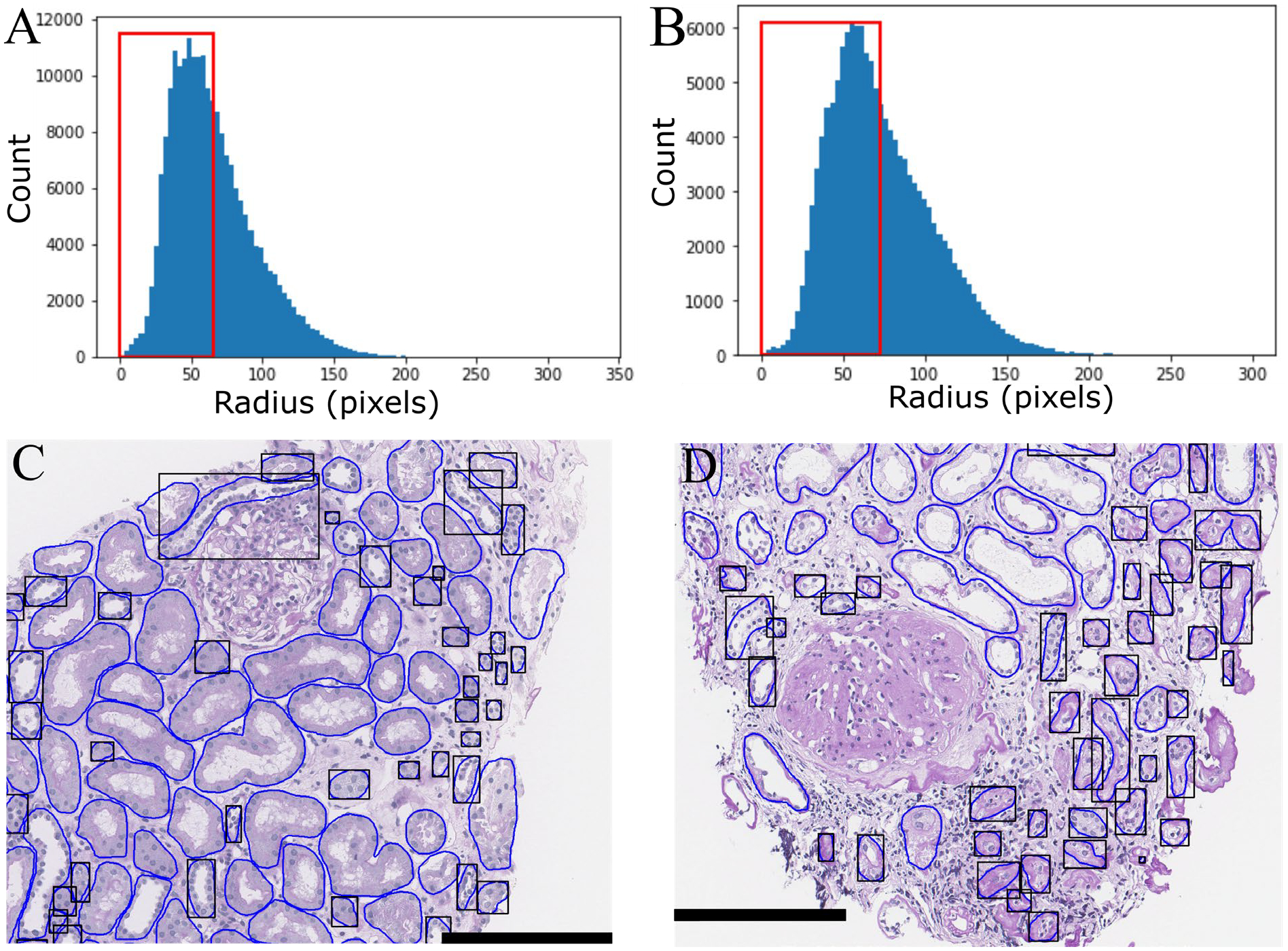
To detect the tubules in kidney biopsies, a previously trained convolutional panoptic neural network model was utilized ^[8]. The outputs of this model were translated to an XML based annotation file that can be viewed in a whole slide image (WSI) viewer such as Aperio^® ImageScope. The segmented tubular boundaries can be seen as blue outlines in Figure 2.

Figure 2. Visualization of tubules with radius less than the global mean (μ).

Histogram of tubular radii in A) transplant tubules and B) DN tubules (red box - less than μ). Example of C) transplant and d) diabetic nephropathy WSI with black boxes highlighting tubules with radius below μ.

Diameter Measurement.

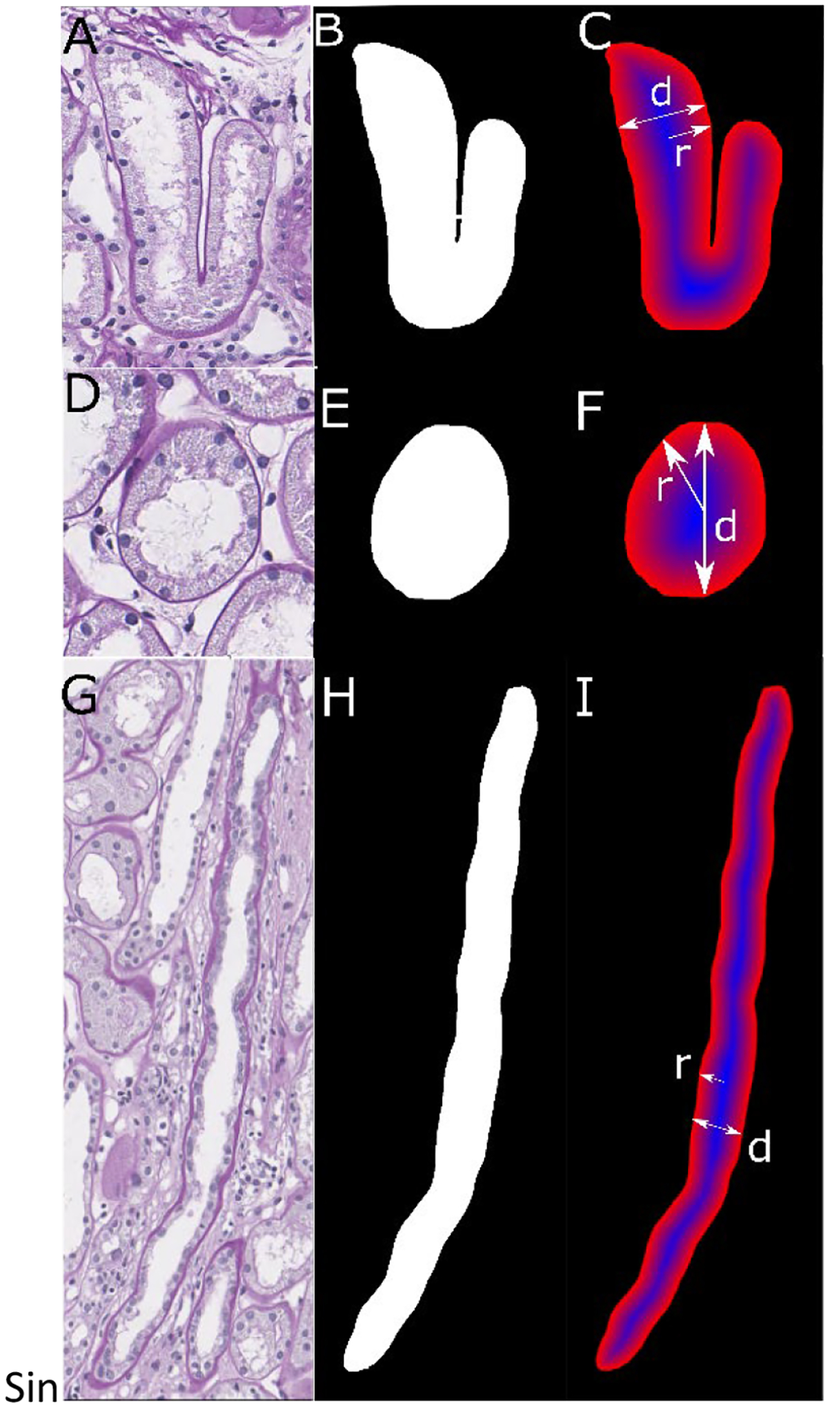
To calculate the tubular radius of tubules with widely variant sectioning profiles, we used the maximum value of the distance transform^[9] of the tubular region. This approximates the radius of the tubule in a generalized fashion regardless of its sectioning angle, as shown in Figure 1. In Figs 1A–C, the radius and diameter area measured for a curved tubule, in Figs. 1D–F, the radius and diameter are measured for a circular tubule, while in Figs 1G–I, the radius and diameter are measured for a straight tubule

Figure 1. Tubular Diameter Measurement.

A) Curved tubule with its B) predicted boundary and the C) distance transformation (blue: high values, red: low values). D) Circular tubule with E) predicted boundary and F) distance transformation. G) Straight tubule with H) predicted boundary and I) distance transform of a straight tubule.

Single morphometric isolation.

Each detected tubule (total ~303K) was measured with the 206 digital histomorphometric features. To facilitate investigation of this massive dataspace, we developed an algorithm to highlight tubules in biopsies based on a user specified range in morphometric feature. To demonstrate its utility, we first calculated the mean and standard deviation of the radii of pooled tubules from either diabetic nephropathy (DN) or transplant patients. For the transplant biopsy tubules, the mean radius and standard deviation were found to be μ_t = 73.15 pix / 18.29 microns and σ_t = 31.1 pix / 7.8 microns; for the diabetic patients, μ_d = 65.24 pix / 16.31 microns and σ_d = 29.8 / 7.45 microns. Using these values and the automatically segmented boundaries, we isolated tubules with radius less than the global mean inside the original WSI. Figs. 2A and 2B respectively show the histogram of measured radii for transplant and DN tubules. Figs. 2C (transplant) and 2D (DN) respectively show the corresponding tubules of Figs. 2A and 2B mapped back to two individual WSI. The highlighted tubules primarily correspond to tubular atrophy. This tool could easily be repurposed on a set of control tissues to define a reference range of ‘normal/healthy’ tubular morphometrics.

Multimorphometric tubular isolation.

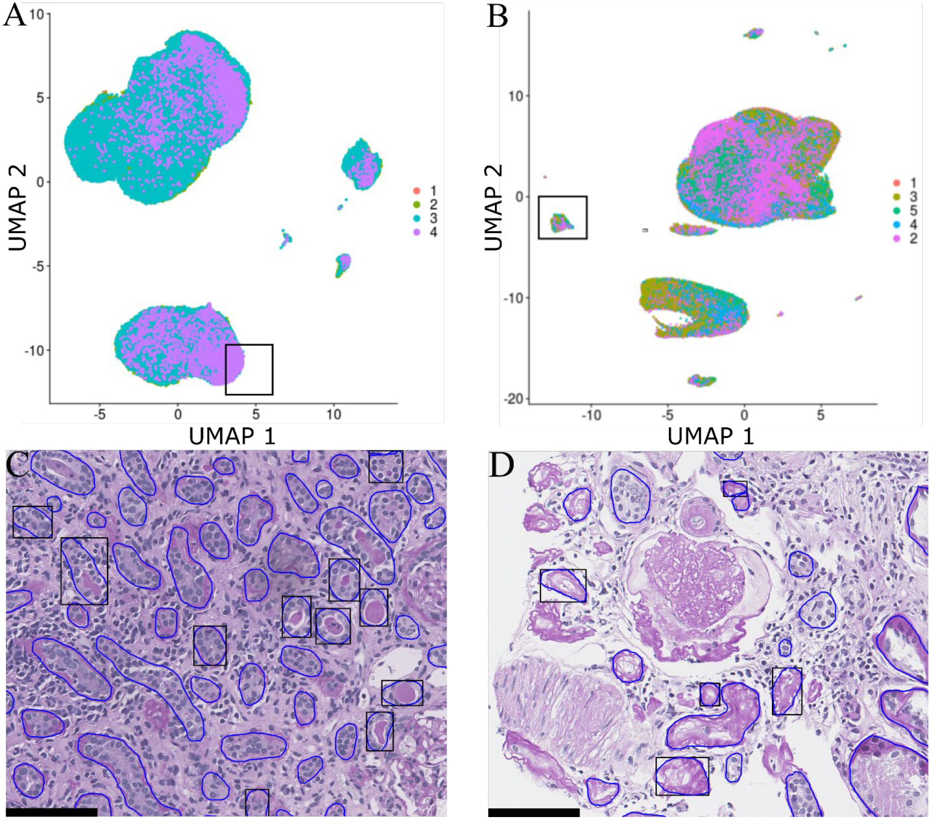
Although individual morphometric measurements are useful, clinical assessments are rarely based on a single morphometric measurement. To further investigate the morphological properties of the tubules accounting for multiple features, we expanded our tool to highlight tubules based on user-selected coordinates of a uniform manifold approximation and projection (UMAP) dimensionality reduction plot^[10]. Fig. 3A shows the reduction plot for the 206 features of tubules in transplant kidney biopsies, whereas Fig. 3B shows the reduction plot for the morphological features extracted from each tubule of native DN kidney. Color labels correspond to the recorded CKD stage of the patient from which the tubule was extracted. In each reduced dimensional space, a number of distinct and separate point clouds can be observed, implying the existence of several distinct morphological signatures. Moreover, within each point cloud, there is a variable distribution of structures from CKD stages, such as CKD 4 tubules preferring to cluster on the northern end of the largest cluster in Figure 3A. Black boxes in Figs. 3A and 3B were selected manually by the user, and the tubules in this cluster were mapped back onto the WSI with black outlines in Figs. 3C and 3D. Points identified in Figs. 3A/3C appear to correspond to smaller radius tubules, the majority of which display casts in their lumen. Points identified in Figs. 3B/3D appear to correspond to severely atrophic tubules without any observable nuclei (Fig. 3D).

Figure 3. Multimorphometric tubular isolation.

UMAP of extracted A) transplant tubular morphological measurements and B) DN tubular morphological measurements. Example of C) transplant and D) DN kidney with tubules-of-interest (from A and B) highlighted. Numerical labels indicate CKD stage.

III. METHODS

Image data.

WSIs of PAS-stained biopsy sections (2μm thick) from 57 native diabetic kidneys and 30 transplant kidneys were used, as collected for a previous study [8, 11]. All images were scanned with a whole slide scanner (Aperio^®, Leica) at 40x magnification resulting in images with a resolution of 0.25 μm/pixel. Human data collection procedure followed a protocol approved by the Institutional Review Board at University at Buffalo.

Tubular Segmentation.

Tubules were detected with a custom designed convolutional panoptic segmentation network [12]. The network identified a total of 302,696 tubules in the 87 WSIs.

Tubular Features.

The tubular feature measurement process was similar to that published in recent previous work by the authors [11], but expanded and modified for application to tubules. Each individual tubule was sub-compartmentalized using simple color transformations and thresholded into five classes: nuclei, epithelia, lumina, tubular basement membrane (TBM), or intra-tubular PAS objects (PAS stained droplets, apical brush borders, casts, or other PAS stained cellular debris). 206 features were measured on each identified tubule using these sub-components, measuring a number of characteristics such as morphometry, texture, color, and intrastructual and interstructural distances.

To ensure a proper measurement of the tubular diameter regardless of tubular shape or type of cut, we first performed a distance transformation, which calculates, for each pixel foreground pixel, the distance to the nearest background pixel. First, for each pixel, distance to the background in the x direction and y directions is calculated, and the Pythagorean theorem is used on these to yield the magnitude of the vector which points directly to the closet background pixel. Then, each of these vectors describes one inscribed circle centered around every pixel, and therefore, the largest of these would yield a radius which is equivalent to half the diameter of the overall tubule.

Feature dimensional reduction.

Dimensionality reduction was done using the Seurat package^[13]. Image features were first centered and scaled to have zero mean and unit variance. Then, a principal component analysis was performed, and principal dimensions greater than 20 discarded. The remaining 20 PCA dimensions were reduced to two with a UMAP. The points in the UMAP space were then labeled by the CKD stage of their patient of origin.

Tubular feature visualization.

The visualization tool takes as input the list of extracted features and the associated image names for each feature. Each image name corresponds to a unique identifier linking the particular image to the patient from whence it came and the coordinates of the bounding box used to crop the region. These coordinates are converted to a simple XML-based bounding box annotation readable by Aperio^® ImageScope.

IV. CONCLUSION

We have developed a tool to automatically isolate and study tubules based on their histomorphometric qualities. In future works, we will utilize our tools to develop statistical reference ranges of normal tubules, which can be used as a baseline to be compared to diseased tubular morphometry.

REFERENCES

- 1.Farris AB and Colvin RB, Renal interstitial fibrosis: mechanisms and evaluation. Current opinion in nephrology and hypertension, 2012. 21(3): p. 289–300. [DOI] [PMC free article] [PubMed] [Google Scholar]
- 2.Hommos MS and Rule AD, Should We Always Defer Treatment of Kidney Disease When There Is Extensive Interstitial Fibrosis on Biopsy? American journal of nephrology, 2016. 44(4): p. 286–288. [DOI] [PMC free article] [PubMed] [Google Scholar]
- 3.An Y, et al. , Renal histologic changes and the outcome in patients with diabetic nephropathy. Nephrology Dialysis Transplantation, 2014. 30(2): p. 257–266. [DOI] [PubMed] [Google Scholar]
- 4.Shabaka A, Cases-Corona C, and Fernandez-Juarez G, Therapeutic Insights in Chronic Kidney Disease Progression. Frontiers in Medicine, 2021. 8. [DOI] [PMC free article] [PubMed] [Google Scholar]
- 5.Roufosse C, et al. , A 2018 Reference Guide to the Banff Classification of Renal Allograft Pathology. Transplantation, 2018. 102(11): p. 1795–1814. [DOI] [PMC free article] [PubMed] [Google Scholar]
- 6.Barisoni L, et al. , Digital pathology and computational image analysis in nephropathology. Nature Reviews Nephrology, 2020. 16(11): p. 669–685. [DOI] [PMC free article] [PubMed] [Google Scholar]
- 7.Acs B, Rantalainen M, and Hartman J, Artificial intelligence as the next step towards precision pathology. Journal of Internal Medicine, 2020. 288(1): p. 62–81. [DOI] [PubMed] [Google Scholar]
- 8.Ginley B, et al. , Automated Computational Detection of Interstitial Fibrosis, Tubular Atrophy, and Glomerulosclerosis. J Am Soc Nephrol, 2021. 32(4): p. 837–50. [DOI] [PMC free article] [PubMed] [Google Scholar]
- 9.Fabbri R, et al. , 2D Euclidean distance transform algorithms: A comparative survey. ACM Comput. Surv, 2008. 40(1): p. Article 2. [Google Scholar]
- 10.Becht E, et al. , Dimensionality reduction for visualizing single-cell data using UMAP. Nature Biotechnology, 2019. 37(1): p. 38–44. [DOI] [PubMed] [Google Scholar]
- 11.Ginley B, et al. , Computational Segmentation and Classification of Diabetic Glomerulosclerosis. Journal of the American Society of Nephrology, 2019. 30(10): p. 1953–1967. [DOI] [PMC free article] [PubMed] [Google Scholar]
- 12.Lucarelli N, Urinary Proteomic Guided Discovery of Digital Morphologic Biomarkers in Diabetic Nephropathy. 2021, State University of New York at Buffalo: Ann Arbor. p. 52. [Google Scholar]
- 13.Stuart T, et al. , Comprehensive Integration of Single-Cell Data. Cell, 2019. 177(7): p. 1888–1902.e21. [DOI] [PMC free article] [PubMed] [Google Scholar]