Abstract
Rectal temperature measurement (RTM) from crime scenes is an important parameter for temperature-based time of death estimation (TDE). Various influential variables exist in TDE methods like the uncertainty in thermal and environmental parameters. Although RTM depends in particular on the location of measurement position, this relationship has never been investigated separately. The presented study fills this gap using Finite Element (FE) simulations of body cooling. A manually meshed coarse human FE model and an FE geometry model developed from the CT scan of a male corpse are used for TDE sensitivity analysis. The coarse model is considered with and without a support structure of moist soil. As there is no clear definition of ideal rectal temperature measurement location for TDE, possible variations in RTM location (RTML) are considered based on anatomy and forensic practice. The maximum variation of TDE caused by RTML changes is investigated via FE simulation. Moreover, the influence of ambient temperature, of FE model change and of the models positioning on a wet soil underground are also discussed. As a general outcome, we notice that maximum TDE deviations of up to ca. 2–3 h due to RTML deviations have to be expected. The direction of maximum influence of RTML change on TDE generally was on the line caudal to cranial.
Supplementary information
The online version contains supplementary material available at 10.1007/s00414-023-03040-y.
Keywords: Temperature-based death time estimation, Heat equation, Finite Element cooling model, Core temperature measurement uncertainty, Death time estimation uncertainty
Introduction
Temperature based death time estimation (TDE) is crucial in homicide investigations. TDE is estimated from core temperature measurement data using the model curve T(t) comprising a priori knowledge of the postmortem rectal temperature decline. The phenomenological approach and the physics-based approach are two different techniques used to generate the model curve T(t). The method of Marshall and Hoare with the Henßge parameters from the Nomogram method (MHH) is a prominent phenomenological approach using a double exponential model with fitted parameters for modeling rectal cooling [1]. Physics-based approaches use the heat transfer equation considering heat exchange mechanisms, cooling conditions and thermal material properties. Finite element (FE) based TDE method (FEM) is a physics-based approach with reasonable computational effort (see e.g. [2–4]). For an extensive overview over temperature based TDE see e.g. [5].
In any TDE method, error quantification is a desideratum as TDE results can lead to acquittal or conviction of suspects. Three different errors exist in FEM such as errors due to space and time discretization, input data errors, and model errors. They lead to the deviation of the TDE value from the actual value. Though several approaches for error estimation exist for TDE e.g. for MHH [6] and for FEM [7] none of them takes into account the uncertainty introduced in TDE due to input data errors caused by variations in the rectal temperature measurement location. The present article tries to close this gap using an FE approach. This does not, however, limit the results to FE TDE methods.
Rectal temperature measurement (RTM) can be performed using approved devices and without the necessity to injure the body. However, there is a certain amount of diversity in the characterization of the measurement locus in forensic literature. In early well-known TDE studies [8, 9], it is reported a 3 – 4 inches [7 – 10 cm] insertion depth for RTM. Marshall and Hoare [10] mention the relationship between the liver and rectum temperature. Henßge [11, 12] states that the insertion depth for RTM should be at least 8 cm from the musculus sphincter ani. In [11] Henßge estimates the precision of rectal temperature measurement to be about “ + -2 °C”. Further, Henßge [13] emphasized the usage of linear, rigid and not very flexible thermometers to achieve an insertion depth without applying force. He also recommends a temperature measurement at the mesenteric root in the lower left abdomen additional to the temperature measurement in the deep abdominal space [14]. Moreover, Henßge advises the thermometer to be inserted in the rectum as deep as possible without applying any force [15]. Indeed, a lot of discrepancy in rectal temperature measurement location exists in literature, so it is necessary to study its effects on TDE. Hence, this motivates a sensitivity analysis of TDE with respect to measurement locus.
The study was executed with participation of the Institute of Legal Medicine (IRM) at the University Hospital Jena of the Friedrich-Schiller-University Jena and of the Zuse Institute Berlin (ZIB), an interdisciplinary research institute for applied mathematics and data-intensive high-performance computing.
Additional computation results are presented in the Supplementary Information (SI) associated with the electronic edition of the article available via the website of the journal.
Method
Finite element model
Background information on numerically solving partial differential equations and on FE simulation can be found e.g. in [16].
For one exemplary case of human corpse with a given CT-scan, two different methods were used to generate FE models. In one of the methods, the FE Model (CTM) was developed from the segmentation of a CT scanned human body and in the other, the human body was manually approximated by hexahedral elements (see e.g. [2, 17]). Two variants of this manually generated model were constructed: One model (CM) is floating freely in air and a copy (CMS) of CM is laying firmly on a wet soil substrate. Detailed simulations of physical heat transfer processes generated the rectal temperature curves T(t). The corpse cooling was computed in all of the FE models based on the well known heat transfer Eq. (1), a partial differential equation where c is the specific heat capacity, ρ the mass density, and κ the heat conductivity of the tissue:
| 1 |
Heat transfer from the body to the environment across the skin due to convection and surface-to-ambient radiation was captured by a Robin boundary condition with effective heat transfer coefficient γ as given in Eqs. (2), (3) (see e.g. [7]):
| 2 |
| 3 |
Here, TA is the ambient temperature, h is the heat transfer coefficient, ε is the emissivity and σ is the Stefan-Boltzmann constant. In the CTM developed from the CT scan of a human body, the initial temperature field T0 defined at time t = 0 satisfies Pennes’ Bio-Heat-Transfer-Equation (BHTE) [18]
| 4 |
where ρbcb is the heat capacity of blood, w is tissue perfusion, and Tcore is the body core temperature.
In the manually developed FE model CM, the initial temperature field T0 is defined with a gradient between core and outside elements as in [2] referring to physiology literature.
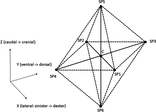
For reliable comparison between the different models, the equivalent effective heat transfer coefficient was applied to the CTM corresponding to the convection and radiation terms applied on CMS and CM. The model curves T(t) were sampled at the designated nodes C and SPRk (k = 1,…6) corresponding to the anatomical RTM locations (RTML). The point C was placed at the intended measurement location in the respective FE model, whereas the six points SPRk (k = 1,…,6) lay on the vertices of an octahedron with radius R. The SPRk were defined to represent possible locations of a misplaced temperature sensor. If no confusion can arise about the value of R the SPRk are abbreviated SPi.
Our results consist of maximum deviations DMAXM comparing two cooling curves computed at two locations of RTM’s in a specified FE model M = CTM, CM, CMS. The distance DMAXM is defined between the cooling curves TC(t) and TSPi(t) at the center point C of a measurement point octahedron (see Fig. 4) of radius R and at its vertices SPRk (k = 1, …, 6). We also computed differences DMAXM1,M2: = DMAXM1 – DMAXM2 of those maximum deviations for two pairs (CM-CMS and CM-CTM) of different FE models (M1, M2) for all C – SPRi pairs. All computations were performed for different constant ambient temperatures TA and for different octahedra radii R. We also performed all of the computations for each of four Q-ranges, where the first three are Henßges Q-ranges (see e.g. [15]).
Fig. 4.
Central position C and six additional measurement positions (SPRk =) SPk (k = 1,…,6) in X, Y and Z direction in CTM, CMS, CM model at different radii R = 0.5 cm, 1 cm, 2 cm from center position C
CT meshed FE model CTM
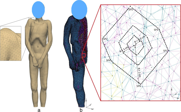
All of the modeling work done on the CT meshed FE model CTM was performed at the Zuse Institute Berlin (ZIB). The CT scan of a male corpse of length L = 1.74 m and weight M = 62 kg was segmented in the software AMIRA and the segmented data was converted into an FE model, comprising of 961,234 tetrahedral elements, via the FE-program Kaskade (see e.g. [19]), an in-house code of ZIB. As depicted in Fig. 1, the feet of the corpse were not included in the model and the weight, size and volume of the whole model were scaled according to the scanned corpse dimensions. The segmentation of different body parts was carried out using differences in density and location of different tissue types like bone, fat, bladder, kidney, abdomen, liver, heart, lungs and muscle as seen in Table 1 in the Appendix.. In CTM, skin tissue was not segmented separately from the subcutaneous fat tissue since skin tissue was assumed to have a negligible effect on the TDE. Hence, the skin material properties were not considered in CTM.
Fig. 1.
a: CT Meshed male corpse model with magnified mesh detail. b: Right half view of CTM model with magnified measurement location showing measurement points C, SPk (k = 1,…,6) in three different octahedra of radii R = 0.5 cm, 1 cm, 2 cm. For the octahedra see Fig. 4. Only the contour lines of the octahedra are shown for clarity
Table 1.
Material properties used in CTM, CM and CMS model [Mall 2005A]
| CTM, CM and CMS model | |||
|---|---|---|---|
| Property | Conductivity | Capacity | Density |
| Unit | W/mK | J/kgK | Kg/m3 |
| Skin | 0.47 | 3680 | 1085 |
| Fat | 0.21 | 2300 | 920 |
| Muscle | 0.51 | 3800 | 1085 |
| Bone | 0.75 | 1700 | 1357 |
| Brain | 0.49 | 3850 | 1080 |
| Face | 0.51 | 3245 | 1056 |
| Neck | 0.48 | 3363 | 1006 |
| Median intestinal Organs | 0.47 | 3375 | 1033 |
| Lungs | 0.28 | 3520 | 560 |
| Stomach | 0.48 | 3730 | 1080 |
| Abdomen | 0.46 | 3346 | 933 |
| Bladder | 0.49 | 3350 | 1008 |
| Kidney | 0.39 | 3158 | 1026 |
| Fat back | 0.21 | 2300 | 920 |
| Wet soil | 2 | 2200 | 1900 |
Coarse meshed FE model CM
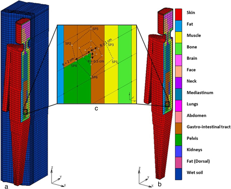
Our coarse meshed FE model CM was already described in several publications [2, 3, 20, 21]. Its mesh was manually constructed using the FE preprocessor Mentat. It consists of approx. 12,000 nodes in approx. 8300 hexahedral elements with trilinear shape functions. The model contains numerous compartments (see Fig. 2) standing for distinct anatomical structures of the body.
Fig. 2.
a: Coarse model lying on a support structure (CMS), b: Coarse model without support structure (CM), c: Detailed view of measurement points C, SP1,….,SP6 along different radii R = 0.5 cm, 1 cm, 2 cm. For the octahedra see Fig. 4. Only the contour lines of the octahedra are shown for clarity
Our standard FE model of length L = 1.64 m and mass M = 64 kg was scaled geometrically to a length of L’ = 1.74 m and weight of M’ = 62 kg, corresponding to the male reference body of our study. The scaling factors are defined as in the Eqs. (5) and (6) where k1 is linear 1-dim scaling along the body length axis and k2 is linear 2-dim dilation in the transverse plane [2].
| 5 |
| 6 |
Generation and scaling of FE mesh and post-processing were performed in MSC’s pre- and post-processing tool Mentat.
Further, to investigate the TDE sensitivity on more complex boundary conditions favoring thermal energy transfer from the body core in dorsal direction, a supporting structure or floor is modeled with an hexagonal FE mesh as shown in Fig. 2a. The FE model lies on its back on the support structure defined, presumably causing large differences between C-temperature and temperature at SP4 or SP3, i.e. along y direction. The support structure is defined with the thermal properties of wet soil such as thermal conductivity c = 2 W/m2K, specific heat κ = 2200 J/kgK, density ρ = 1900 kg/m3 [22] and emissivity ε = 0.95. The coarse model laying on its back on the support structure is abbreviated CMS, whereas the coarse model without support structure is named CM (see Fig. 2c). CMS and CM were scaled to the same height and weight as CTM. This will eliminate the influence of weight on the body cooling.
Definition of measurement positions C and SPRk
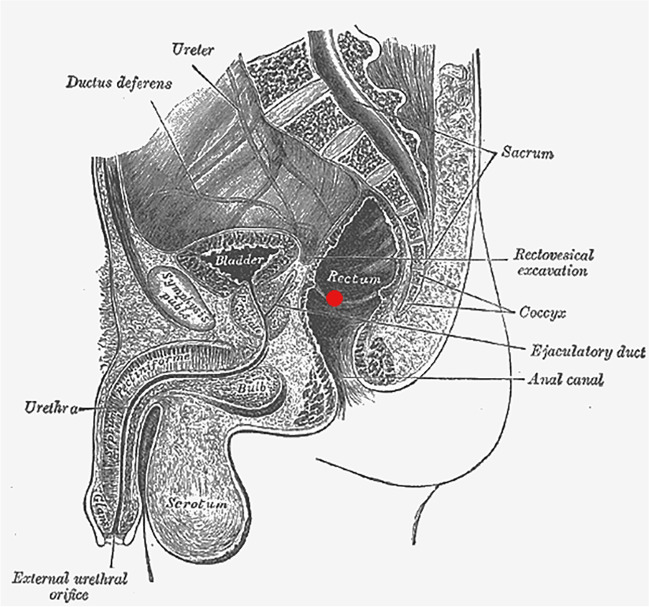
TDE estimations are usually based on a single RTM. Hence, the measurement position is subject to variations due to different anatomies, thermometer angles and insertion depth. An approximate ideal measurement position can be specified from anatomy including forensic knowledge on measurement locations used in practice. The central position C for our measurements was determined in the pars ampullaris of the rectum near the incisura transversalis, which is the passage from pars ampullaris to the pars sacralis of the rectum (Fig. 3).
Fig. 3.
Anatomical sketch depicting ideal measurement location [23]
Additional measurement positions SPRk (k = 1, …,6) for our sensitivity studies were chosen in spatial x, y and z direction at distances (octahedral radii) R = 0.5 cm, 1 cm, 2 cm from the central measurement position C. For each fixed distance R six additional measurement locations SPRk were established. The six additional measurement positions SPRk form an octahedron with the central point C in its middle. The schematic sketch representing the additional positions in the model was illustrated in Fig. 4.
The anatomical position of additional measurement points in CTM are described as follows: SP1 lies in the center of abdomen surrounded by abdomen tissues, SP3 lies nearby bone, SP4 lies in the center of abdomen, SP6 lies very near to abdomen. Figure 1b shows the anatomical positions of measurement points in CTM. Similarly, the anatomical position of additional measurement points in CMS and CM are depicted in Fig. 2c, which helps to identify the position of additional measurement points. SP1 lies lateral from C in positive X direction. Due to CM’s left–right symmetry the temperature value at SP2 is equal to the temperature at SP1. The points SP2, SP3, SP5 lie in the gastrointestinal tract. SP6 and SP4 lie on the border between gastrointestinal tract and pelvis.
Simulation
The CT-generated model CTM was imported from the FE research code Kaskade 7 [19] into the commercial MSC-Marc Mentat FE system and the material parameters are defined as given in Table 1 of [2] (see Table 1 in the Appendix). The same material properties were used also for CMS and CM models. The initial temperature field T0(r) at the time of death on the body was calculated via the Pennes’ Bio-Heat-Transfer-Equation BHTE on the original CTM model [18]. The field T0(r) was approximated by 10 discrete node sets corresponding to 10 discrete temperatures in the converted version of CTM. In the CMS and CM models, the initial temperature was defined according to [2] where it was taken from physiological textbooks. The simulation is carried out for three different constant ambient temperatures TA = 5° C, 15° C, 25° C. The convection and radiation parameters in CTM were defined by the effective heat transfer coefficient γ = 4∙ε∙σ TA3 [7] and the calculated values in increasing order of TA = 5° C, 15° C, 25° C are γ = 7.93 W/m2K, 8.45 W/m2K, 9 W/m2K. In CMS and CM, a convection coefficient of h = 3.3 W/m2 K is applied [2]. Radiation view factors in the CMS and CM models were computed by Monte-Carlo-simulation [2]. Although the method of defining boundary conditions differs between CTM and CM models, it was found that the linearization of the radiation term applied in CTM has negligible effect on the cooling curve [7]. A sparse direct algorithm in MSC-Marc 2020 and adaptive time stepping with maximum allowed temperature change of 1°K and 0.1 s initial time step were used.
Quantification of TDE deviations
TDE deviation from the central position C to any position SPRk is quantified by the maximum distance DMAX between the respective cooling curves, which is defined in this section. Let the time interval [a, b] be given during body cooling which starts at 0 h and let a = 1 h be the left point and b = 45 h be the right point of our interval. Let further T1(t) and T2(t) be two cooling curves defined on the interval [0, b]. Evaluation of the cooling curve distances started at a > 0 h for reasons of numerical stability. The ambient temperature TA is assumed constant in space and time outside the body. The reference curve TR(t) for two cooling curves T1(t) and T2(t) is constructed as the pointwise mean of T1(t) and T2(t):
| 7 |
Let T0: = TR(0) be the initial temperature at the center point C. Now the reference curve TR(t) can be normalized to the function Q(t) taking values in the real number’s interval [0, 1]:
| 8 |
This makes it possible to define the Q-intervals Q1 to Q4 (where Q1, Q2, Q3 correspond to Henßge’s [15] normed temperature ranges for tolerance radii) and their left and right boundaries q0, …, q4 by:
| 9 |
| 10 |
Assuming TR(t) to be strictly monotonically decreasing, we can uniquely map the Q-interval boundaries qn to the respective temperature values TR(4-n).
| 11 |
Since the two cooling curves T1 and T2 are monotonically decreasing it is possible to define their inverse curves t1, t2, called the (absolute) time since death (TSD) estimation result curves w.r.t. the cooling curves T1, T2 on the domain [TMIN,TMAX] which is the range of the reference curve TR on the temperature axis by:
| 12 |
| 13 |
The time functions t1, t2 are frequently concatenated with the reference curve TR, thus giving t1(TR(t)), t2(TR(t)) in the following definitions. For short those concatenations will be abbreviated t1(t), t2(t). If the point t in time is clear, we will even write t1, t2. We will now quantify the distance between the cooling curves T1 and T2, which are actually constructed as distances between the inverse curves t1 and t2. The reason for this construction lies in our primal interest in time differences because our research’s number one target is time since death. All of the temperature curve distance measures are constructed using the (time oriented!) maximum distance DMAX(T1,T2) between two cooling curves T1 and T2, which is shown here for continuous functions first. The maximum domain of the reference curve TR on the time axis is the interval [tMIN,tMAX] which is taken therefore as the domain for maximum-finding in our definition:
| 14 |
We will now consider the equivalent of the definition (14) in terms of real measured temperature curves Ti(t). Each curve Ti(t) is represented as a finite series of real measurement values (Ti1, …, TiN) on a finite (regular) grid of time values (t1, …, tN) which is the same for both of the curves. The first point t1 of the time grid is identical to the starting time of cooling computation, while the last point tN marks the end of the cooling computation interval. To provide a joint domain of definition for both our inverted temperature curves TR−1 we define:
| 15 |
| 16 |
Now we have constructed the range of our reference curve TR(t). The limits of its domain of definition [tMIN,tMAX] were computed:
| 17 |
| 18 |
Let K be a natural number and let (t1, …, tK) be a regular time grid on the interval [tMIN,tMAX] with t1: = tMIN and tK: = tMAX. This provides the equidistant sampling points for the final definition of the functions ti(TR(t)). Let further be (T1, …, TK) the corresponding temperature grid with T1 ≤ … ≤ TK and Tk: = TR(tk) for all k = 1, …, K and TK: = TMAX. The time grid’s width Δt is:
| 19 |
Let further be tqn the inverse image of TRn under the reference function TR for all n = 0, …, 4:
| 20 |
The five points tqn on the time scale constitute the endpoints of four time intervals tQ1, …, tQ4:
| 21 |
We will redefine our measure (14) quantifying the distance between the cooling curves T1 and T2 in terms of the real samples (t1, …, tK) and (Ti1, …, TiK). The distance measure is the distance DMAX (T1, T2). It is defined in a global version on the whole time interval [tMIN, tMAX] and in four local ones residing on one of the intersections tQj ∩ [tMIN, tMAX] on the time axis each. For all 1 ≤ i ≤ 4 the number of tk lying in tQj ∩ [tMIN, tMAX] is denoted by Ki.
The (absolute global) maximum distance DMAX(T1, T2) is defined as:
| 22 |
while the (absolute) Qi-local maximum distance DMAX,Qi(T1, T2) is defined for i = 1, …, 4:
| 23 |
Results
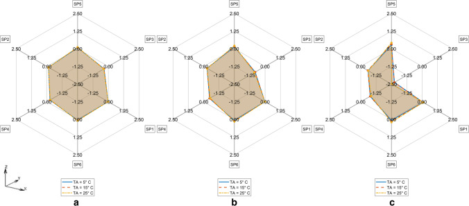
In a first step we evaluated the results for the direction in space (X,Y,Z as in Fig. 4), where the largest TDE-deviation value DMAX caused by RTML -variation was seen. Interestingly, this maximum direction depended neither on the ambient temperature TA = 5 °C, 15 °C, 25 °C nor on the octahedron radius R = 0.5 cm, 1 cm, 2 cm. The FE-model chosen makes the only difference. Therefore we get the following list of directions for maximum DMAX caused by RTML-variation:
CM: Z caudal—cranial
CTM: Y ventral—dorsal
CMS: Y ventral—dorsal
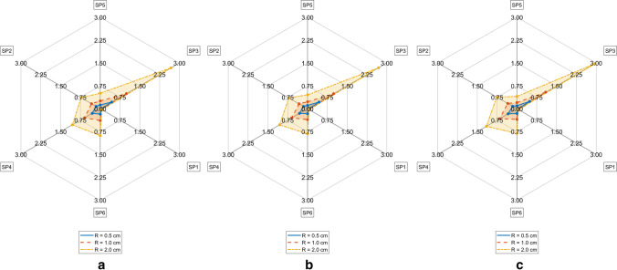
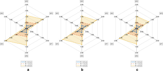
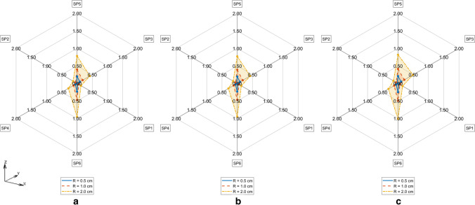
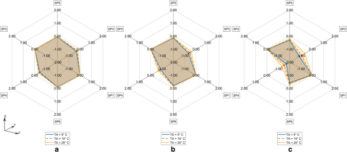
TDE deviations measured by DMAXM on the FE model M = CTM, CMS, CM respectively depending on ambient temperature TA and measurement radius R are represented in Figs. 5, 6 and 7. The differences of TDE deviations DMAXM1,M2 on the model pairs (M1, M2) = (CM, CTM), (CM, CMS) as depicted in Figs. 8 and 9 were calculated as follows: DMAXCM,C™ = DMAXCM—DMAXC™ and DMAXCM,CMS = DMAXCM—DMAXCMS.
Fig. 5.
TDE deviation in DMAX for CTM for R = 0.5 cm (Solid line), R = 1.0 cm (Dashed line), R = 2 cm (Dash-dotted line) a. TA = 5° C, b. TA = 15° C, c. TA = 25° C
Fig. 6.
TDE deviation in DMAX for CMS for R = 0.5 cm (Solid line), R = 1.0 cm (Dashed line), R = 2 cm (Dash-dotted line) a. TA = 5° C, b. TA = 15° C, c. TA = 25° C
Fig. 7.
TDE deviation in DMAX for CM for R = 0.5 cm (Solid line), R = 1.0 cm (Dashed line), R = 2 cm (Dash-dotted line) a. TA = 5° C, b. TA = 15° C, c. TA = 25° C
Fig. 8.
Difference in TDE deviation in DMAX between CM vs CMS model for TA = 5° C (Solid line), TA = 15° C (Dashed line), TA = 25° C (Dash-dotted line) for a. R = 0.5 cm, b. R = 1 cm, c. R = 2 cm
Fig. 9.
Difference in TDE deviation in DMAX between CM vs CTM for TA = 5° C (Solid line), TA = 15° C (Dashed line), TA = 25° C (Dash-dotted line) a. R = 0.5 cm, b. R = 1 cm, c. R = 2 cm
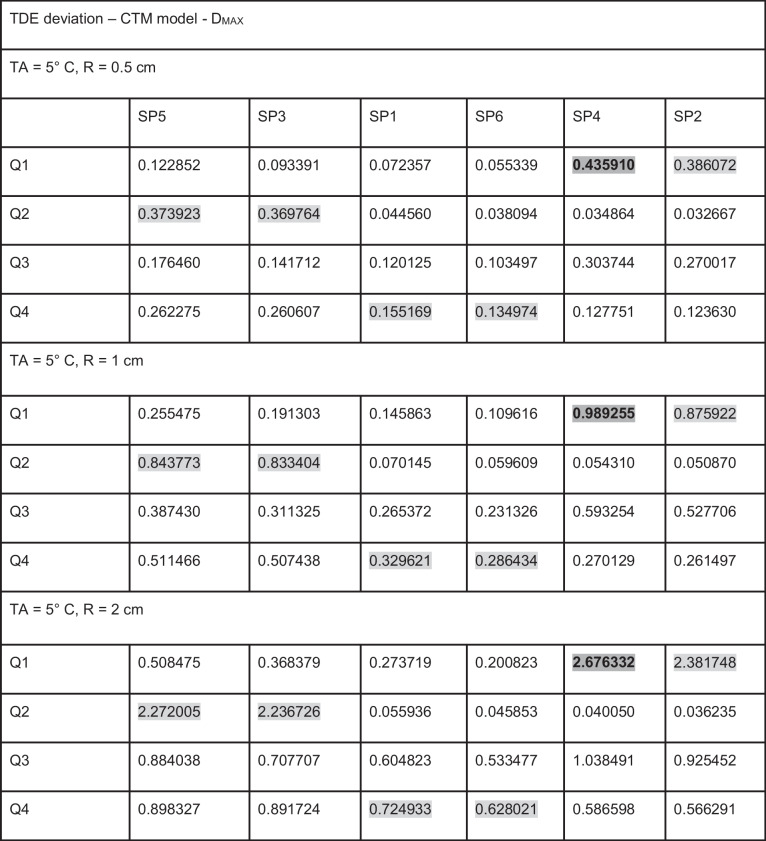
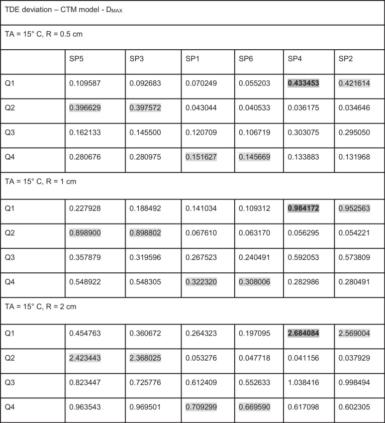
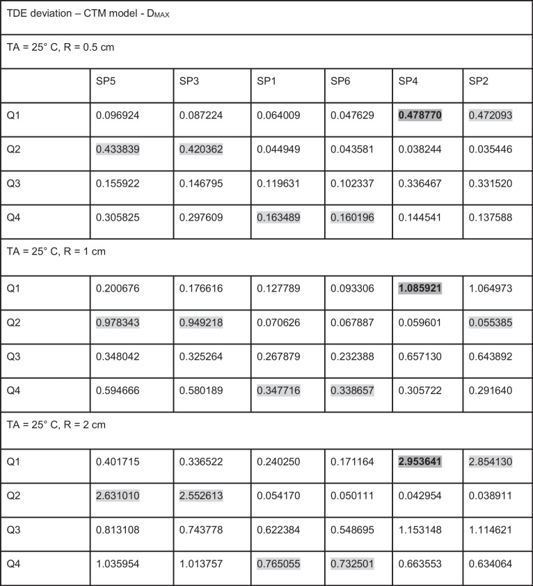
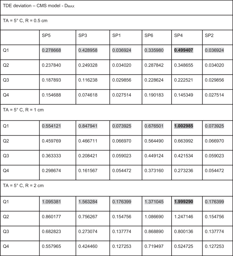
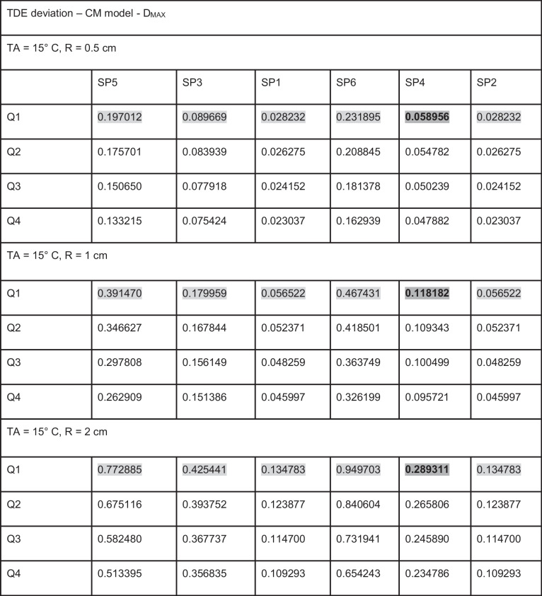
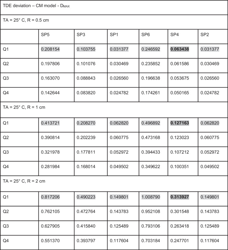
TDE deviations DMAX,QiM at various measurement points SPRk (k = 1, …,6) evaluated against C in M = CTM, CMS, CM at various ambient temperatures TA and Q regions are shown in Tables 2, 3, 4, 5, 6, 7, 8, 9 and 10 in the Appendix. The RTML SPRk (k = 1, …,6) in Tables 2, 3, 4, 5, 6, 7, 8, 9 and 10 are arranged corresponding to clockwise order in Figs. 5, 6, 7, 8 and 9. Browsing the tables the following regularities can be noticed:
For all of the models M = CTM, CMS, CM, and for each fixed combination of TA and R the maximum value of DMAX,Qi over all Qi and over all SPRk is taken at SPR4 in Q1 (dark grey, fat print in Tables 2, 3, 4, 5, 6, 7, 8, 9 and 10).
For M = CM, CMS, and for each fixed combination of TA, R, SPRk the maximum value of DMAX,Qi over all Qi is taken in Q1 (light grey in Tables 5, 6, 7, 8, 9 and 10).
- For M = CTM, and for each fixed combination of TA, R, the maxima of DMAX,Qi for fixed SPRk are as follows:
-
aIn the SPR5- and in the SPR3-column at Q2
-
bIn the SPR1- and in the SPR6-column at Q4
-
cIn the SPR2-column at Q1
-
a
For M = CM, CMS, and for each fixed combination of TA, R, SPRk the DMAX,Qi values are declining with rising index i of Qi. The only exception occurs for M = CMS in Table 7 and TA = 25 °C at R = 1 cm and R = 2 cm at SPR3: where we see DMAX,Qi rise from Q3 to Q4
Table 2.
TDE deviation DMAXM in M = CTM at TA = 5° C. Maximum value for fixed R and fixed SPRk: light grey, maximum value for fixed R over all SPRk: fat print, dark grey
Table 3.
TDE deviation DMAXM in M = CTM at TA = 15° C. Maximum value for fixed R and fixed SPRk: light grey, maximum value for fixed R over all SPRk: fat print, dark grey
Table 4.
TDE deviation DMAXM in M = CTM at TA = 25° C. Maximum value for fixed R and fixed SPRk: light grey, maximum value for fixed R over all SPRk: fat print, dark grey
Table 5.
TDE deviation DMAXM in M = CMS at TA = 5° C. Maximum value for fixed R and fixed SPRk: light grey, maximum value for fixed R over all SPRk: fat print, dark grey
Table 6.
TDE deviation DMAXM in M = CMS at TA = 15° C. Maximum value for fixed R and fixed SPRk: light grey, maximum value for fixed R over all SPRk: fat print, dark grey
Table 7.
TDE deviation DMAXM in M = CMS at TA = 25° C. Maximum value for fixed R and fixed SPRk: light grey, maximum value for fixed R over all SPRk: fat print, dark grey
Table 8.
TDE deviation DMAXM in M = CM at TA = 5° C. Maximum value for fixed R and fixed SPRk: light grey, maximum value for fixed R over all SPRk: fat print, dark grey
Table 9.
TDE deviation DMAXM in M = CM at TA = 15° C. Maximum value for fixed R and fixed SPRk: light grey, maximum value for fixed R over all SPRk: fat print, dark grey
Table 10.
TDE deviation DMAXM in M = CM at TA = 25° C. Maximum value for fixed R and fixed SPRk: light grey, maximum value for fixed R over all SPRk: fat print, dark grey
Results concerning relative TDE difference distances and distances based on the L2-norm instead of the MAX norm are presented in the electronic SI.
Discussion
Multiple analysis was carried out to determine the TDE error caused by measurement locus variations for the different FE-model types such as CTM, CM, CMS using maximum distance DMAX.
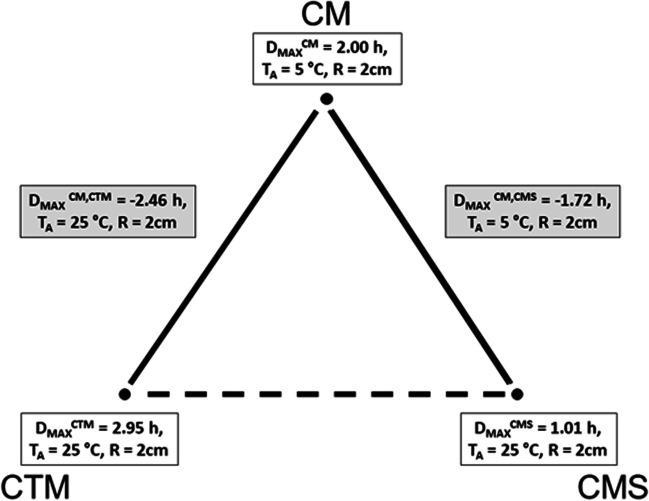
Our simulation results show maximum TDE deviations DMAX with respect to variations in RTML up to 2 cm in the order of magnitude of 2 to 3 h. Comparing to other influences like variations in ambient temperature TA (see [6, 7]), initial body core temperature T0 (see [20]), etc. the TDE deviations of 2 to 3 h are not negligible and can cause considerable errors in TDE. Our RTML-caused TDE deviation results DMAX lie within the 95% confidence interval of Henßge [15]. For the first Q interval, Henßge gives a value of 2.8 h for standard as well as for non-standard conditions, which is in the same order of our TDE deviations caused by variations of the RTML.
The maximum TDE deviation DMAX in CTM and in CMS is observed in the dorsal–ventral axis Y (Fig. 5: SP3, Fig. 6: SP4).
This may be due to the close vicinity of RTML to backbone tissue. A higher value of thermal conductivity of bone tissue of k = 0.75 W/m2K compared to the conductivity of other soft tissue types, will result in higher temperature gradient in the line C – nearest backbone parts. Similarly, a higher temperature gradient occurs along the Y: dorsal–ventral SP3—C—SP4 axis in case of CMS due to high conductivity of substrate. Only in CM the axis SP6 – C – SP5 (Z: caudal—cranial) shows the highest DMAX values (see Fig. 7). This may be the case because the CM model lacks the high conductivity substrate the CMS model contains. Other differences between CM and the other models might as well be part of the explanation: The CM shows symmetric anatomical structures with respect to the mid sagittal plane while the CTM does not. Furthermore, the CTM has a much finer discretization than the CM and a varying spatial tissue distribution due to the manual versus the CT-based mesh generation in CM and CTM respectively. Concerning the FE-meshwidth, we found only a minor effect on the TDE difference results as well as [7]. Hence, the TDE differences between the CM and the CTM can hardly be explained from differences in the discretization order.
The only difference between CMS and CM is that in CMS, the coarse-meshed human model lies on a discretized structure with wet soil’s thermal properties whereas CM consists of a coarse-meshed human model floating freely (like CTM model) in air without contact to other solid structures. The difference DMAXCM,CMS compares CM vs. CMS model thus considering the influence of the support structure on the sensitivity of TDE against RTML variation. Like in forensic scenarios heat transfer from the corpse to support with high conductivity and / or heat capacity will increase heat flux through the models support-contact faces. Assuming a support with comparably low thermal conductivity, like a highly insulated mattress, a decrease in heat flux will be the consequence. The influence of different support materials on TDE was investigated in [21, 24]. Thermal properties of the support were also considered in the Henßge model, where supports with high thermal conductivities are taken into account by increasing the correction factor and vice versa (see e.g. [15]). Our results show that the influence of different supports on TDE sensitivity with respect to RTML variations need to be considered because they may lead to differences in temperature gradients which transform to differences in TDE.
The ambient temperature TA influences the TDE sensitivity against RTML variations in the CMS model in such a way that the TDE deviation increases with decrease in TA. Possibly, this effect is due to the presence of the support structure along the dorsal–ventral axis (Y axis (SP4 – C – SP3)), which increases the rate of heat transfer. The initial temperature of the support structure was always set to the ambient temperature TA. In contrast, looking at the TDE difference DMAXCM,C™ between DMAX in CM and in CTM, there is nearly no influence of ambient temperature TA. Apparently, the influence of TA on TDE difference is more profound when the support structure is present.
Concerning the influence of RTML variation radius R, the maximum TDE deviation DMAX increases with increase in R in CTM, CMS and CM. This is due to greater Euclidean distance of measurement points from the actual measurement point, which is translated via temperature gradient to greater DMAX.
Figure 10 gives the overview of the maximum TDE deviation by RTML variation evaluated by DMAX for CTM, CMS and CM with respect to ambient temperature TA and measurement variation radius R.
Fig. 10.
Maximum TDE deviation in DMAX in CTM, CMS and CM model
The evaluation of the Qi-located TDE distances DMAX,QiM between SPRk and C yields the following results: Firstly measurement location errors in the ventral –dorsal axis Y seem to cause the most severe deviations of TDE (see (R1)). For the coarse model regardless of whether there is a wet soil substrate (M = CMS) or not (M = CM) the DMAX,Qi values essentially decline with rising Q-index I that is for rising cooling times (see (R4)). Since the latter regularity is not repeated by the CT-generated model CTM, we infer this to be an artificial effect caused by the unrealistic high symmetry and regularity of the ‘hand-crafted’ FE models CMS and CM. Generally the effect of RTML errors on TDE seems to be highest at short times after death (see (R1)). Time evolution of TDE errors due to RTML variations thus correspond to the well known effect, that initial temperature deviations lead to high TDE errors during short times p.m. but are later damped to a low constant basic amount. This is shown in [6] for MHH – TDE but may be generalized. Moreover it is consistent with [7].
There are limitations of the current study. Firstly, we used a simulation-based approach for TDE estimation and RTML variation. A validation of our results on experimental measurements with real corpses was not realized. Measurements using corpses of recently deceased – aside from rare availability of such corpses—are difficult to carry out and especially a reproducible RTML variation is nearly impossible. However, in former studies the CM was calibrated and validated based on some experimental measurements published in [21]. Due to the physics-based approach, both the CM and the CTM should be suitable to carry out parameter variations in terms of RTML variation. Secondly, we only use three different models with normal body mass index. Cooling scenarios with more complex boundary conditions, like adipose corpses, clothing and coverings, etc. were not considered although these factors can influence TDE deviation as CMS depicts. Since varying all those boundary conditions would exceed the scope of one research article, those sensitivity studies are left for future research.
Conclusions
TDE variations caused by RTML deviations may be a source of error in legal medicine TDE since they may reach a magnitude of 2–3 h. A possible consequence for legal medicine applied research could be to investigate methods and devices for reproducible RTML determination.
Electronic supplementary material
Below is the link to the electronic supplementary material.
Acknowledgements
The present study is part of a project funded by the Deutsche Forschungsgemeinschaft DFG with the reference numbers MA 2501/4-1 (Prof. Dr. Gita Mall) and WE 2937/10-1 (Dr. Martin Weiser).
Appendix
Table 1
Table 2
Table 3
Table 4
Table 5
Table 6
Table 7
Table 8
Table 9
Table 10
Authors contributions
Study design and milestone discussions: All authors. CT-segmentation: ZIB authors. FE model CTM generation: ZIB authors, CTM migration: All authors. CMS generation: IRM authors. FE computations: J. Ulrich, J. Shanmugam, H. Muggenthaler. Distance measure computations: J. Shanmugam, M. Hubig. Output interpretation/presentation: J. Shanmugam, M. Hubig, H. Muggenthaler, J. Ulrich. Paper written/corrected: J. Shanmugam, M. Hubig, H. Muggenthaler. Paper reading / corrections: All authors.
Funding
Open Access funding enabled and organized by Projekt DEAL.
Material and/or code availability
The individual CT scan used in the current study is not publicly available. Each single slice is linked to a DICOM-file containing experiment parameter data and sensible case information. The program code is available from the corresponding author on reasonable request.
Declarations
Ethical approval
No living or deceased humans nor living or dead animals were directly involved in the study. Written consents of the CTM-subject’s kinship for the CT scan shown in the article were not needed since the body was confiscated by the local prosecution who directed the CT scan for investigations.
Competing interests
The authors herewith disclose financial or non-financial interests that are directly or indirectly related to the work.
Footnotes
Publisher's note
Springer Nature remains neutral with regard to jurisdictional claims in published maps and institutional affiliations.
References
- 1.Henßge C (2016) 6.1 Basics and application of the ‘nomogram method’ at the scene. In: Madea B (ed) (2016) Estimation of the Time Since Death, 3rd edn. CNC Press Taylor & Francis Routledge, Boca Raton FL
- 2.Mall G, Eisenmenger W. Estimation of time since death by heat-flow Finite-Element model. Part I: method, model, calibration and validation. Leg Med. 2005;7(1):1–14. doi: 10.1016/j.legalmed.2004.06.006. [DOI] [PubMed] [Google Scholar]
- 3.Mall G, Eisenmenger W. Estimation of time since death by heat-flow Finite-Element model part II: application to non-standard cooling conditions and preliminary results in practical casework. Leg Med. 2005;7(2):69–80. doi: 10.1016/j.legalmed.2004.06.007. [DOI] [PubMed] [Google Scholar]
- 4.Schenkl S, Muggenthaler H, Hubig M, Erdmann B, Weiser M, Zachow S, Heinrich A, Güttler F, Teichgräber U, Mall G. Automatic CT-based finite element model generation for temperature-based death time estimation: feasibility study and sensitivity analysis. Intl J Leg Med. 2017;131(3):699–712. doi: 10.1007/s00414-016-1523-0. [DOI] [PubMed] [Google Scholar]
- 5.Madea B, editor. Estimation of the Time Since Death. 3. Boca Raton FL: CNC Press Taylor & Francis Routledge; 2016. [Google Scholar]
- 6.Hubig M, Muggenthaler H, Mall G. Influence of measurement errors on temperature-based death time determination. Int J Legal Med. 2011;125:503–517. doi: 10.1007/s00414-010-0453-5. [DOI] [PubMed] [Google Scholar]
- 7.Weiser M, Erdmann B, Schenkl S, Muggenthaler H, Hubig M, Mall G, Zachow S. Uncertainty in temperature-based determination of time of death. Heat Mass Transf. 2018;54:2815–2826. doi: 10.1007/s00231-018-2324-4. [DOI] [Google Scholar]
- 8.De Saram GSW, De Webster G, Kathirgamatamby N. Post-mortem temperature and the time of death. J Crim Law Criminol. 1955;46(2):562–577. doi: 10.2307/1139735. [DOI] [Google Scholar]
- 9.Marshall TK, Hoare FE. Estimating the time of death. The rectal cooling after death and its mathematical expression. J Forensic Sci. 1962;7:56–81. [Google Scholar]
- 10.Marshall TK, Hoare FE. Estimating the time of death. The use of the cooling formula in the study of post-mortem body cooling. J Forensic Sci. 1962;7:189–210. [Google Scholar]
- 11.Henßge C. Die Präzision von Todeszeitschätzungen durch die mathematische Beschreibung der rektalen Leichenabkühlung. Z Rechtsmedizin. 1979;83:49–67. doi: 10.1007/BF00201311. [DOI] [PubMed] [Google Scholar]
- 12.Henßge C, Madea B (1988) Methoden zur Bestimmung der Todeszeit an Leichen, 1st edn. Schmidt-Römhild, Lübeck, Verlag Schmidt-Römhild, Lübeck, Germany, p 288
- 13.Henßge C, Brinkmann B, Püschel K. Todeszeitbestimmung durch Rektaltemperaturmessungen bei Wassersuspension der Leiche. Z Rechtsmedizin. 1984;92:255–276. doi: 10.1007/BF00200284. [DOI] [PubMed] [Google Scholar]
- 14.Henßge C. Todeszeitschätzungen durch die mathematische Beschreibung der rektalen Leichenabkühlung unter verschiedenen Abkühlbedingungen. Z Rechtsmedizin. 1981;87:147–178. doi: 10.1007/BF00204763. [DOI] [PubMed] [Google Scholar]
- 15.Henßge C. Todeszeitbestimmung an Leichen. Rechtsmedizin. 2002;12:112–131. doi: 10.1007/s00194-002-0136-8. [DOI] [Google Scholar]
- 16.Deuflhard P, Weiser M. Adaptive numerical solution of PDEs. Berlin: De Gruyter; 2012. [Google Scholar]
- 17.Hubig M, Muggenthaler H, Mall G (2016) 6.2 Finite element method in temperature-based death time determination. In: Madea B (ed) (2016) Estimation of the Time Since Death, 3rd edn. CNC Press Taylor & Francis Routledge, Boca Raton FL
- 18.Pennes HH. Analysis of tissue and arterial blood temperatures in the resting human forearm. J Appl Physiol. 1948;1(2):93–122. doi: 10.1152/jappl.1948.1.2.93. [DOI] [PubMed] [Google Scholar]
- 19.Götschel S, Schiela A, Weiser M. Kaskade 7 - a flexible finite element toolbox. Comp Math Appl. 2021;81:444–458. doi: 10.1016/j.camwa.2020.02.011. [DOI] [Google Scholar]
- 20.Muggenthaler H, Hubig M, Schenkl S, Mall G. Influence of hypo- and hyperthermia on death time estimation - A simulation study. Leg Med. 2017;28:10–14. doi: 10.1016/j.legalmed.2017.06.005. [DOI] [PubMed] [Google Scholar]
- 21.Muggenthaler H, Hubig M, Schenkl S, Niederegger S, Mall G. Calibration and parameter variation using a finite element model for death time estimation: the influence of the substrate. Leg Med. 2017;25:23–28. doi: 10.1016/j.legalmed.2016.12.007. [DOI] [PubMed] [Google Scholar]
- 22.Cengel YA, Ghajar AJ. Heat and Mass Transfer – Fundamentals and Applications. 5. New York: McGraw-Hill; 2014. [Google Scholar]
- 23.Gray H (1918) Anatomy of Human Body, 1st edn. Lea & Febiger, Philadelphia, Retrieved from Library of Congress. https://lccn.loc.gov/18017427. Accessed 17 Oct 2022
- 24.Baumann F (2020) Impact of contact surfaces on the death estimation. Master Thesis, Technische Universität Berlin, p 69
Associated Data
This section collects any data citations, data availability statements, or supplementary materials included in this article.
Supplementary Materials
Data Availability Statement
The individual CT scan used in the current study is not publicly available. Each single slice is linked to a DICOM-file containing experiment parameter data and sensible case information. The program code is available from the corresponding author on reasonable request.


