A systematic review of automated segmentation of 3D computed‐tomography scans for volumetric body composition analysis

Abstract

Automated computed tomography (CT) scan segmentation (labelling of pixels according to tissue type) is now possible. This technique is being adapted to achieve three‐dimensional (3D) segmentation of CT scans, opposed to single L3‐slice alone. This systematic review evaluates feasibility and accuracy of automated segmentation of 3D CT scans for volumetric body composition (BC) analysis, as well as current limitations and pitfalls clinicians and researchers should be aware of. OVID Medline, Embase and grey literature databases up to October 2021 were searched. Original studies investigating automated skeletal muscle, visceral and subcutaneous AT segmentation from CT were included. Seven of the 92 studies met inclusion criteria. Variation existed in expertise and numbers of humans performing ground‐truth segmentations used to train algorithms. There was heterogeneity in patient characteristics, pathology and CT phases that segmentation algorithms were developed upon. Reporting of anatomical CT coverage varied, with confusing terminology. Six studies covered volumetric regional slabs rather than the whole body. One study stated the use of whole‐body CT, but it was not clear whether this truly meant head‐to‐fingertip‐to‐toe. Two studies used conventional computer algorithms. The latter five used deep learning (DL), an artificial intelligence technique where algorithms are similarly organized to brain neuronal pathways. Six of seven reported excellent segmentation performance (Dice similarity coefficients > 0.9 per tissue). Internal testing on unseen scans was performed for only four of seven algorithms, whilst only three were tested externally. Trained DL algorithms achieved full CT segmentation in 12 to 75 s versus 25 min for non‐DL techniques. DL enables opportunistic, rapid and automated volumetric BC analysis of CT performed for clinical indications. However, most CT scans do not cover head‐to‐fingertip‐to‐toe; further research must validate using common CT regions to estimate true whole‐body BC, with direct comparison to single lumbar slice. Due to successes of DL, we expect progressive numbers of algorithms to materialize in addition to the seven discussed in this paper. Researchers and clinicians in the field of BC must therefore be aware of pitfalls. High Dice similarity coefficients do not inform the degree to which BC tissues may be under‐ or overestimated and nor does it inform on algorithm precision. Consensus is needed to define accuracy and precision standards for ground‐truth labelling. Creation of a large international, multicentre common CT dataset with BC ground‐truth labels from multiple experts could be a robust solution.

Background

At a tissue level, body composition (BC) measures the proportions and quantities of adipose tissue (AT), skeletal muscle (SM), organs and bone. There is strong evidence that abnormal BC phenotypes predict cancer outcomes. In particular, sarcopenia predicts survival and postoperative complications in head and neck, breast, lung and gastrointestinal tract malignancies, ¹ , ² , ³ , ⁴ , ⁵ as well as recurrence. ⁶ , ⁷ , ⁸ , ⁹ Combinations of abnormal BC have further lethality; cancer patients with sarcopenic obesity are at even greater mortality risk. ¹⁰ , ¹¹

In order for BC to routinely feature in treatment planning, two broad criteria need to be achieved: an effective time‐critical treatment for abnormal BC proven to improve outcomes and an accurate and convenient method of measurement. This systematic review will explore how technological advancement may achieve the latter.

Segmentation is key to quantifying BC from cross‐sectional imaging such as computed tomography (CT) or magnetic resonance imaging (MRI). Figure 1 depicts a magnified CT image to demonstrate that such digital scans are made of a large number of pixels. Segmentation is an image processing term referring to labelling of each individual pixel (or voxels which are 3D pixels) according to tissue or organ. ¹² Since CT and MRI are frequently used in clinical practice, segmentation has allowed for opportunistic BC assessment in clinical cohorts without need for further patient investigation. ¹³

Figure 1.

A magnified CT image depicting the individual pixels constituting the scan. Segmentation is the process of labelling each pixel as a specific tissue; skeletal muscle (SM), visceral (VAT) and subcutaneous adipose tissue (SAT) in this case. Image (A) depicts a single, two‐dimensional axial CT slice taken from the abdominal region. Image (B) shows all regions of SAT (blue), VAT (yellow), and SM (red) labelled according to tissue type. Image (C) magnifies an area containing psoas SM, VAT and left kidney. The individual grayscale pixels are visible. Image (D) shows segmentation of each individual pixel according to body composition tissue type. The kidney is left unlabelled. Counting the total number of pixels belonging to a tissue type with the pixel scale will produce a surface of SM, VAT or AT for this 2D slice. Applying this process to voxels in a 3D region would quantify volume. Images generated from Data Analysis Facility Suite v3.6 by Voronoi.

Excluding cadaveric studies, true in vivo reference standards for measuring BC at tissue level are by volumetric segmentation and quantification of three‐dimensional (3D) cross‐sectional imaging spanning the full body. ¹⁴ It was demonstrated over 30 years ago that CT and MRI respectively could be used to quantify regional and total body SM and AT volumes. ¹⁵ , ¹⁶ A 1998 validation study confirmed that MRI and CT segmentation were equally accurate at quantifying SM and AT compared with cadaveric measurements, with high reproducibility. ¹⁷ However, volumetric segmentation could only be previously manually performed, ¹⁸ , ¹⁹ which was a laborious and highly time‐consuming process. Furthermore, the majority of clinically derived CT are regional anatomical scans, rather than true head‐to‐fingertip‐to‐toe whole body images. For example, most cancer staging CT cover chest, abdomen, and pelvis, omitting SM and AT from the head, neck, upper and lower limbs. Thus, a commonly adopted approach has been a two‐dimensional (2D) segmentation of a single axial L3 vertebral slice. ¹⁰ , ¹¹ , ²⁰ , ²¹ , ²² , ²³ A landmark study, Shen et al. showed surface areas obtained from a single axial MRI slice highly correlated with total body SM and AT volume. ¹⁹ This concept was then validated for CT within a cancer cohort using a single L3 axial slice. ²⁴ Thus, segmentation of a single axial L3 slice became de facto for studying BC in cancer patient cohorts with an abdominal CT. The L3‐skeletal muscle index (SMI) was then introduced, where SM‐surface area is normalized for height (cm²/m²), allowing for group comparisons. The importance of single lumbar slice BC analysis cannot be understated. It has been seminal to research on the interplay between BC and cancer for the past two decades.

However, advances in computing and artificial intelligence (AI) now feasibly allow volumetric regional BC analysis from 3D cross‐sectional imaging as an alternative to single slice. Whilst limited by anatomical extents of scans performed in clinical practice, this may have advantages due to the greater proportion of total body volume captured. Whilst automated 3D segmentation of MRI for BC analysis exists, CT has more widespread use in clinical practice particularly within cancer. Furthermore, to our knowledge, this is currently limited to research scans with specific acquisition protocols differing to clinical imaging as exemplified by the UK Biobank Imaging Study. ²⁵ , ²⁶ , ²⁷ , ²⁸ Therefore, this systematic review focuses on automated segmentation of 3D clinical CT scans for regional volumetric BC analysis and aims to evaluate accuracy, feasibility and current limitations and pitfalls.

Methods

Search methodology

This systematic review was conducted in accordance with Preferred Reporting Items for Systematic Reviews and Meta‐analyses (PRISMA) guidelines. ²⁹ Searches were conducted on OVID Medline, 1946 to October 2021; Embase, 1974 to October 2021; grey literature databases including arXiv, bioRxiv, medRxiv and Mednar. Primary search terms consisted of whole body, full body, total body, three‐dimensional, 3D, segmentation, body composition, body tissue composition, sarcopenia, automated, automatic, AI, machine learning, deep learning, neural network, computed tomography and CT.

We included original studies trialling an automated method for segmenting volumetric CT scans, with the ability to quantify the following three BC parameters: visceral adipose tissue (VAT), subcutaneous adipose tissue (SAT) and SM. We did not enforce bone segmentation as a criterion because dual energy X‐ray absorptiometry (DEXA) exists as a well‐established technique. Only studies using manually segmented scans for training and performance evaluation were included. There was no discrimination between healthy and diseased participants. Exclusion criteria included articles without a full paper; reviews or editorials; modalities other than CT; lack of manually segmented ground‐truth labels; non‐English language; cadaveric or animal studies; paediatric patients <18 years old; inability to segment all three aforementioned BC parameters. Where two or more studies originated from the same group with the former acting as preliminary work for the latter segmentation strategy, only the most up‐to‐date publication was included.

Selection process

The selection and extraction processes were conducted using Covidence. ³⁰ Screening of abstracts and titles was conducted by two authors (D. M. and I. D.). Full text reviews were then performed again by D. M. and I. D. against our inclusion/exclusion criteria, with included studies proceeding to extraction via a pre‐determined proforma.

Assessing study quality

As we anticipated many studies would involve AI, interpretations were formed from Faes et al., who provide a basis for clinicians to critically appraise machine learning studies. ³¹ The points considered are specified, along with technical terminology explanations.

Algorithm training

Sample size analysis for minimum required CT scans for training and testing should be considered and described.

Ground‐truth originally refers to images or measurements identified by maps, air photography or satellites that can be physically confirmed by on‐ground observation. ³² , ³³ It is now a common AI term referring to data accepted to be true, by direct observation or measurement. This provides a reference standard to test the prediction performance of a machine or human observer. For example, previous studies assessed the accuracy of radiologists' identification of malignant lymph nodes in rectal cancer from preoperative MRI. The ground‐truth to compare radiological assessment against, would be the postoperative histopathology results. ³⁴ In the case of automated segmentation of BC tissue, ground‐truth would be CT scans with pixels/voxels pre‐labelled according to SM or AT by humans with appropriate expertise. In the context of CT segmentation, gold standard for expertise would be fully trained board‐certified radiologists. At a minimum, this takes 5 years, or between 5 and 7 years of postgraduate training in North America and Europe, respectively. This should be described in detail, ideally with more than one labeller enabling interobserver agreement analysis.

Algorithm testing

Within grayscale CT scans, a pixel is the smallest unit of a digital image containing an attenuation value, with a voxel being its 3D equivalent. In machine learning, validation is data used to fine‐tune an algorithm after training. Testing refers to the process of evaluating model performance. Metrics used by the AI community to evaluate a predictive algorithm's performance may initially be confusing or unfamiliar to clinicians but are similar to equations derived from contingency tables for evaluating performance of medical diagnostic tests. Figure 2 demonstrates this within the context of evaluating an algorithm's performance for automated labelling of CT pixels as SM.

Figure 2.

A schematic representation of Dice similarity coefficient for skeletal muscle segmentation (labelling) in a 10 × 10 pixel region of interest within a CT scan. The human expert manually labels eight of the nine pixels as skeletal muscle (red) in (A). Automated segmentation of the same pixels by a machine algorithm (B) has achieved 16 true positive, one false negative, five false positive, and 78 true negative muscle labels. This is summarized by the contingency table (C), allowing for calculation of sensitivity, specificity, PPV, NPV and Dice coefficient by the specified equations.

The Dice similarity coefficient (DSC, also known as the Sørensen–Dice index or Dice coefficient) is the most common metric for assessing performance of automated segmentation algorithms and will be assessed for each study. This statistical tool measures similarity between two sets of data summarized by the following equation:

$$\frac{2*\left(\text{True Positives}\right)}{\left(\left(2*\text{True Positives}\right)+\text{False Positives}+\text{False Negatives}\right)}$$

Using SM as an example, it measures the degree of overlap between the pixels labelled as SM by ground‐truth human observer versus the automated algorithm within a specified region of pixels. The score ranges from zero to one, with one denoting perfect segmentation performance. It is the most widely used method for evaluating segmentation performance as it penalizes for both false positives and negatives within a single metric. ³⁵ However, DSC is limited in informing on the over‐segmentation or under‐segmentation of a BC tissue. ³⁶ Thus, contingency tables should ideally be reported alongside which allows positive predictive value (PPV) and sensitivity to be calculated. These are known as precision and recall in AI, but because precision confusingly has another meaning in medical applications, the traditional terms PPV and sensitivity will be used. In Figure 2, the PPV is noticeably lower than DSC whilst sensitivity is higher, implying the algorithm tends to excessively label pixels as SM. Due to the large number of pixels not belonging to a BC tissue within a CT slice or volume, metrics such as specificity and negative predictive value have limited meaning in segmentation evaluation as the result remains high despite increasing levels of false negative labels. ³⁵ Thus, we will review papers for their reporting of DSC, sensitivity and PPV.

There also should be a clear split in training and test scans. Scans used for training and fine‐tuning can be seen by the algorithm, whilst testing scans should be unseen; that is, there should be no overlap between training and testing scan datasets.

Algorithm generalizability

For an algorithm to be useful in the real‐world, the training set data should capture real‐world clinical heterogeneity seen in CT. Patient variables include age, sex, anthropometry and disease status, whilst scan variables including anatomical coverage, axial slice thickness and the use of contrast.

Algorithms should undergo external testing with ‘temporally and/or preferably geographically’ separate datasets from different institutions, and ideally by independent investigators. ³¹

Results

Search outcome

After removal of duplicates, 92 studies were identified for screening and 23 articles progressed to full text review. As depicted in Figure 3, seven studies were included for data extraction, and synthesis after exclusion criteria was applied. ³⁷ , ³⁸ , ³⁹ , ⁴⁰ , ⁴¹ , ⁴² , ⁴³ Tables 1 and 2 summarize the study characteristics and details.

Figure 3.

PRISMA diagram.

Table 1.

Study characteristics

Year, country	Public availability of segmentation technique	Scan indication selection	Age (years)	Sex M%:F%	BMI	Scan modality	Authors' description of extent of CT	Sample size calculation	Training sample	Unseen internal testing sample	Unseen external testing sample	Segmentation method
2018, USA 37	Open source	Unknown	Unknown	Unknown	Unknown	CT (contrast unknown)	Abdomen and pelvis	Nil	20	20	20	Multi‐atlas segmentation
2019, France 38	Under development	Post cancer (type unknown) treatment with full response	56.9 ± 12.8	50:50	27.1 ± 4.6	PET‐CT	Eyes to ischium	Nil	30	Nil	Nil	Multi‐atlas segmentation
2020, USA 39	Unavailable	50% non‐cancers for training 50% cancers for testing	Unknown	Unknown	Unknown	CT (oral ± intravenous contrast)	Thorax, abdomen, pelvis	Nil	30	Nil	30	Deep learning, Hounsfield thresholding, morphological smoothing
2020, USA 40	Unavailable	81.6% ‘minimally abnormal’ 18.4% cancer (type unknown)	31‐83	66:34	17.3‐38.3	PET‐CT	15 mm above lung apices to inferior ischial tuberosities	Nil	38	Nil	Nil	Deep learning
2021, Canada 41	Commercially available	Unknown	Unknown	Unknown	Unknown	CT (contrast unknown)	Whole body, unclear	Nil	Unknown	50	Nil	Deep learning
2021, Germany 42	Unavailable	Unselected	62.6 ± 9.5	60:40	Unknown	CT (intravenous contrast)	Abdomen	Nil	40	10	Nil	Deep learning
2021, S. Korea 43	Commercially available	Training and internal testing: early lung cancer External testing: non‐cancer and head/neck cancers	62.3 ± 13.3	40:60	23.1 ± 3.9	CT (non‐contrast)	Head to lower arm and mid‐thigh	Nil	90	10	64 + 522 (KURE)	Deep learning

Table 2.

Study details

Reference	Body composition components	Cross‐validation	Data‐augmenting	Ground‐truth: labeller	Ground‐truth: Intra/inter‐ observer variation	Ground‐truth: generation	Dice coefficient	Sensitivity	Positive predictive value	Algorithm speed
Hu et al. 37	SAT; VAT; SM; psoas	Not specified	No	‘Single experienced rater’	Unknown	Manual segmentation; but slices every other 5 cm	SM 0.854 VAT 0.887 SAT 0.933	Unknown	Unknown	Unknown
Decazes et al. 38	SAT; VAT; SM	Leave‐one‐out cross validation	No	‘Radiology expert’	Unknown	Manual segmentation; leave one out method	SM 0.95 TAT 1.00 VAT 0.97	Unknown	Unknown	25 min
Fu et al. 39	SAT; VAT; SM; Bone	Five‐fold cross validation	No	Two radiology residents, one physics resident, 2–4 years CT review experience. Supervised by qualified radiologist	Unknown	Manual segmentation	SM 0.95 VAT 0.94 SAT 0.96	SM 0.95 VAT 0.98 SAT 0.98	SM 0.96 VAT 0.91 SAT 0.93	Unknown
Liu et al. 40	SAT; VAT; SM	Five‐fold cross validation	No	‘Well trained operators’ verified by board certified radiologist	Unknown	Semi‐automated and manual whole body segmentation	SM 0.924 VAT 0.942 SAT 0.974	SM 0.934 VAT 0.937 SAT 0.972	SM 0.919 VAT 0.950 SAT 0.977	12 s
Ma et al. 41	SAT; VAT; SM; Bone	Not specified	No	‘A team of trained anatomists’	Unknown	Manual segmentation	SM 0.974 VAT 0.960 SAT 0.996	Unknown	Unknown	Unknown
Koitka et al. 42	SAT; VAT; SM; Bone	Five‐fold cross validation	Yes	Unknown	Unknown	Manual segmentation not of entire volume; every 5th slice only	SM 0.933 SAT 0.962	Unknown	Unknown	Unknown
Lee et al. 43	SAT; VAT; SM; Bone	Not specified	No	Training: one technician, one radiology resident (3 year experience), one qualified radiologist (15 year experience) Testing: three qualified radiologists (5 to 8 year experience)	Unknown	Manual segmentation	Internal SM 0.981 VAT 0.951 SAT 0.971 External SM 0.903‐0.992 VAT 0.924‐0.989 SAT 0.941‐0.997	Internal SM 0.985 VAT 0.943 SAT 0.962 External SM 0.868‐0.995 VAT 0.918‐0.991 SAT 0.968‐0.996	Internal SM 0.978 VAT 0.960 SAT 0.980 External SM 0.918‐0.991 VAT 0.932‐0.987 SAT 0.916‐0.997	75 s

SAT, subcutaneous adipose tissue; SM, skeletal muscle; VAT, visceral adipose tissue.

Study design and input data characteristics

All studies were retrospective and non‐interventional. Scans were performed solely for clinical purposes and retrieved from clinical repositories in six studies; one study did not specify the source. ⁴¹ One study obtained scans specifically from a cancer cohort. ³⁸ Two studies sourced a mixture of cancer patients and non‐cancer patients. ³⁹ , ⁴⁰ , ⁴³ One study specifically did not consider scan indication, ⁴² and two scans did not describe indication. ³⁷ , ⁴⁴ One study excluded scans with altered postoperative anatomy ⁴⁰ ; no other studies specified any further imaging selection criteria based on quality or artefact. There was further heterogeneity regarding patient characteristics of the derived scans, with the male:female ratio ranging from 40:60 to 87:13 and three studies ³⁷ , ³⁹ , ⁴¹ not defining the sex at all. Only three of eight studies defined BMI. ³⁸ , ⁴⁰ , ⁴³ CT scan acquisitions were a mixture of contrast, non‐contrast and positron‐emission‐tomography (PET).

Sample size calculation was not reported in the methodology in any study.

Anatomical extent of computed tomography scans

There was both variation and ambiguity regarding CT coverage as shown in Table 1 stating in verbatim the nomenclature used by each paper. Decazes measuring the region between eyes and ischium, and Liu who defined body‐torso as 15 mm superior to the lung apices to inferior border of ischial tuberosities. ³⁸ , ⁴⁰ The remaining studies were not explicit regarding objective the anatomical boundaries delineating whole body, abdomen or pelvis. One study stated whole body coverage without elaboration. ⁴¹ It is unclear if whole body truly means head‐to‐fingertip‐toe, and this terminology ambiguity is further highlighted by Lee initially describing their training scans as whole body before defining this as spanning head to mid‐thigh only. ⁴³

Automated segmentation technique

Multi‐atlas segmentation

As shown in Table 2, the earliest two studies ³⁷ , ³⁸ used multi‐atlas segmentation (MAS). Whilst computer algorithms automated the process, this is not based upon AI. Generally, this involved initially creation of masks (or atlases) of SAT, VAT and SM through manual segmentation of series of training scans. A mask is the binary image produced after labelling pixels/voxels as either belonging or not belonging to a specific tissue type. ⁴⁵ , ⁴⁶ A volume of slices from a novel target CT scan is then brought into spatial correspondence with the pre‐existing selection of atlases, a process termed image registration. The registered pairs of atlas/target CT scans with the highest level of labelled pixel concordance then undergo a process named label fusion, producing an optimal segmentation of either SM, SAT and AT and a quantitative measure.

Deep learning

Machine learning is a subcategory of AI describing an algorithm's ability to uncover and learn complex relationships between variables within a high‐dimensional training dataset in order to predict outputs based on new inputs. This distinguishes it from traditional computing algorithms whereby pre‐determined rules are applied to inputs to generate outputs. Deep learning (DL) is a further subset of machine learning that uses layers of mathematical formulae organized to resemble neuronal pathways of the brain, known as a neural network.

Fu ³⁹ used a combination of DL and post‐processing. Using a neural network, the ventral cavity (defined by the study as thorax, abdomen and pelvis) was segmented. Based upon the premise that SAT and SM lies outside of the cavity whilst VAT lies within, an automated workflow was then applied using image attenuation thresholding and morphological operations. Using five‐fold cross validation across 38 abdominal CT volumes, Liu ⁴⁰ used 23 CT scans to train their own novel neural network named ABCnet to segment body‐torso (thorax, abdomen and pelvis) CT scans. Koitka ⁴² trained a U‐Net 3D architecture to segment abdominal CT scans. To reduce the amount of manual labelling required, every fifth slice was annotated. Using 90 CT volumes, Lee ⁴³ also trained both a U‐Net 2D and 3D network, with the latter segmenting a series of adjacent axial slices as an entire volume as opposed to one slice after another.

Ground‐truth labelling

All studies involved ground‐truth manual labelling of both training and testing scans. However, there was marked variation in the expertise and numbers of labellers. Only Lee et al. had board‐certified radiologists directly performing the labelling (in addition to radiology residents and technicians). ⁴³ The remaining studies either used a ‘single experienced rater’, ³⁷ a ‘radiology expert’, ³⁸ radiology and physics residents, ³⁹ ‘well trained operators’, ⁴⁰ ‘trained anatomists’, ⁴¹ or an unspecified labeller. ⁴² No studies reported intra‐observer, and the papers using more did not appear to analyse interobserver variation.

Training data

For the two studies using non‐DL MAS protocols, 20 to 30 scans appeared to sufficiently train the algorithm, with Decazes and Liu using leave‐one‐out and five‐fold cross validation, respectively. ³⁷ , ³⁸

For the DL studies, training scan quantity ranged from 30 to 90 scans ³⁹ , ⁴⁰ , ⁴² , ⁴³ or unspecified in the case of Ma. ⁴¹ Koitka was the only study to report applying augmentation techniques to artificially increase the size of their training data. ⁴²

Testing

Only two of the seven studies included both unseen internal and external testing; Hu et al. conducted this on 20 extrinsic patient CT scans, ³⁷ whilst Lee et al. ⁴³ validated across three external cohorts of 20, 20 and 24 patients, respectively. Whilst not undertaking unseen internal testing, Fu externally tested on 30 scans.

Four studies included unseen internal testing albeit with significant variation in the quantity of scans used, ranging from 10 to 50. ³⁷ , ⁴¹ , ⁴² , ⁴³ The remaining three studies, Decazes et al., Fu et al. and Liu et al., respectively, employed cross‐validation to simultaneously train and evaluate their technique but did not test on a novel, unseen set of internal or external scans. ³⁸ , ³⁹ , ⁴⁰

Segmentation performance

All ground‐truth labelling was performed manually by trained clinicians, and every study used DSC to evaluate segmentation performance. As shown in Table 2, the five NN‐based studies achieved Dice scores >0.9 for SAT, VAT and SM. ⁴⁰ , ⁴¹ , ⁴² , ⁴³ The MAS‐based Anthoprometer3D by Decazes ³⁸ also achieved this. Three studies ³⁹ , ⁴⁰ , ⁴³ reported sensitivity and PPV; all remained greater than 0.9 with the exception of external testing of SM segmentation in Lee 2021 where sensitivity was 0.868 to 0.995. ⁴³ No studies provided contingency tables quantifying true and false positive or negative labelling for further analysis.

Clinical validation

The first six papers were proof of concept studies. Only the seventh, Lee et al. ⁴³ clinically validated the use of their regional BC analysis method to predict sarcopenia. As previous quantifiable cut‐offs for sarcopenia have been made through cross‐sectional 2D segmentation, novel volumetric parameters were proposed, including waist volumes of SM and AT (inferior margin of 12th rib to superior margin of iliac crest). These volumes were divided by the length of the waist to give average waist surface areas. Average SM waist surface areas were then divided by height² to produce SMI (cm²/m²). AT was standardized by body fat index (cm²/kg). The authors used CT scans from a pre‐existing cohort study of elderly Korean adults investigating the prevalence and outcomes of cardiovascular, musculoskeletal and age‐related diseases. Along with the CT scans, these patients had undergone a combination of functional and bioimpedance analysis to diagnose sarcopenia according to criteria from the Asian Working Group for Sarcopenia. ⁴⁷ , ⁴⁸ After using linear regression to define cut‐offs, authors showed an 82% agreement between sex‐specific average waist SMI and a clinical diagnosis of sarcopenia.

Discussion

There have been previous narrative reviews assessing automated BC segmentation. These have overviewed principles of DL‐driven segmentation, ⁴⁹ , ⁵⁰ included single‐slice only techniques, ⁵¹ , ⁵² or have broadly reviewed advances in segmentation of all organs, lymph nodes, lesions and BC tissues. ⁵² To our knowledge, this is the first systematic review to focus on fully automated volumetric BC analysis from 3D CT scans, specifically relevant for researchers and clinicians interested in opportunistic BC evaluation.

The review shows opportunistic volumetric BC assessment from clinically obtained 3D CT images is now feasible. The use of DL techniques makes the process accurate, automated and fast. A trained neural network could automatically segment full CT scans rapidly; 12 and 75 s respectively in two studies reporting speed ³⁹ , ⁴³ compared with 25 min for a non‐DL algorithm. ³⁸ Furthermore, the above studies have achieved this within a variety of different acquisition protocols (contrast enhanced, non‐contrast and PET) as well as a mix of anatomical coverage. This reflects real‐world heterogeneity that could allow for volumetric BC analysis in a wide range of diseases where CT plays a routine role. However, whilst promising, this review also highlights new dilemmas and limitations posed by this technology for BC researchers to contend with.

Ground‐truth accuracy and precision—Who is an expert?

In order for end‐users to trust automated segmentation algorithms, there must be confidence in the accuracy of ground‐truth labels used for training and testing. ²⁸ Whilst three of seven studies explicitly describe board‐certified radiologists supervising manual segmentation, only in one study were radiologists actually performing the ground‐truth labelling. No studies assessed the intra‐ or inter‐observer variation of the ground‐truth segmentations.

There is a need for a consensus on what constitutes an expert qualified to provide ground‐truth segmentation. A reasonable criterion would be a board‐certified radiologist, but should this exclude non‐radiologists from producing ground‐truth BC labels? Accuracy refers to how close a value is to a true or accepted result. ⁵³ Thus, a solution could be for potential ground‐truth labellers within a study to compare their labels tested against a board‐certified radiologist experienced in segmentation, meeting a pre‐determined minimum level of inter‐observer agreement. A similar concept is currently being used in the CIPHER Study (UK Cohort Study to Investigate the prevention of Parastomal Hernia). Non‐radiologists (surgical residents) are being recruited to be CT scan assessors, providing they meet a minimum agreement level (90%) with a radiologist on a series of test scans. ⁵⁴ Potential labellers should also meet a minimum level of precision, the ability to reproduce a similar result on repeated attempts. ⁵⁵ For DEXA, minimum precision standards exist defined by the International Society for Clinical Densitometry; 3%, and 2% for fat and lean mass, respectively. Technologists performing BC from DEXA are required to undergo to confirm precision by testing and retesting their BC measurements on an initial DEXA and repeat scan on a same group of patients. ⁵⁶ Similarly, intra‐observer variation of ground‐truth labellers for an algorithm should be assessed and reported by manually relabelling a selection of scans twice.

Since the completion of this review period for these seven papers, more sophisticated methods of ground‐truth creation have been applied in automated 3D CT segmentation for BC analysis. Alavi published BodySegAi, a DL‐algorithm capable of volumetric segmentation of CT abdomen/pelvis. Ground‐truth BC labelling was performed by a radiologist, a radiographer and a dietician. The authors then used the STAPLE (simultaneous truth and performance level estimation) algorithm to generate the optimum single ground‐truth by combining segmentations from all three labellers. ⁵⁷ This algorithm originates from neuroradiology as a means of establishing optimal ground‐truth labels from multiple labellers for training of neural networks to segment brain tumours. Briefly, the STAPLE algorithm applies weights to each labeller's manual segmentations, by assessing their accuracy. These weighted labels are then used to produce a final single ground‐truth segmentation. Not only has it been thoroughly internally tested by its pioneer, ⁵⁸ it has been used externally in non‐BC neuroradiological ⁵⁹ , ⁶⁰ and histopathological ⁶¹ datasets for training and testing of DL segmentation models. STAPLE should therefore be considered another optimal standard for CT BC ground‐truth generation.

Algorithm segmentation performance

As it punishes algorithms for false positive and negative labelling and can summarize performance as a single number, DSC is considered a robust metric for evaluating pixel‐by‐pixel labelling performance. This was used in all studies, with DL algorithms reporting scores >0.9 for BC tissues. However, DICE scoring has limitations in terms of clinical translation. Once unified cut‐offs are defined, AI‐driven BC analysis could be used in clinical practice as an aid to sarcopenia and visceral obesity diagnosis. It would thus be crucial to know the relative volume difference of SM or AT: Relative volume difference = $\frac{\mathit{\text{Ground truth volume}}–\mathit{\text{Predicted volume}}}{\mathit{\text{Ground truth volume}}}.$ ⁶² This metric would quantitatively inform the extent to which overestimation or underestimation of may occur, which could cause patients to be misclassified as either having adequate SM volume or having sarcopenia.

Another consideration not interpretable from DSC, PPV or sensitivity is precision (in this meaning, ability to reproduce the same BC quantification) of automated CT segmentation algorithms. This metric is crucial for longitudinal assessments because knowing the least detectible magnitude of change in SM or AT volume allows clinicians to decide whether increases/decreases on follow‐up scans are due to algorithm variation or due to true BC change. This was achieved in DEXA by test and re‐test where the patient undergoes the scan twice, usually in the same session. Whilst acceptable due to DEXA's very low radiation dose (33 times less than a chest X‐ray), this would be unethical with CT (100 times higher than chest X‐ray) on living participants. A solution could lie in the creation of an anthropometric radiographic phantom ⁶³ (artificial objects representing human form and tissue) simulating BC that can be scanned twice in immediate succession. A cadaveric study would also be an option.

Generalizability

A DL‐model's learned methodology for segmenting tissue is highly dependent on training data quality and size. Hence, small scan datasets may insufficiently reflect the heterogeneity of real‐world CT scans in terms of radiological features. Indeed, the majority of studies in this review used only 20 to 40 scans, ³⁷ , ³⁸ , ³⁹ , ⁴⁰ , ⁴² which can lead to overfitting, where the neural network becomes very good at segmenting similar datasets but performs poorly on new, unseen scans. ³¹ The difficulty in generating larger training CT datasets lies not only in the labour and time intensity required for manual pixel labelling on a volumetric scale, but also in finding suitable experts to do so. One solution is data augmentation, where images are manipulated to artificially increase the pool of training scans; only one study reported this. ⁴²

The review highlights deficiency in segmentation performance testing. A 2015 consensus statement from a working group of clinicians and biostatisticians strongly recommended that prediction models for individual diagnosis undergo performance testing on an external dataset. ⁶⁴ A 2019 systematic review and meta‐analysis comparing DL versus clinician performance in medical imaging diagnosis found that only 24% of 82 studies tested their models on an external cohort. ⁶⁵ This is consistent with only two of seven studies demonstrating external testing (albeit with excellent performance) within this review. ³⁷ , ⁴³ Models may demonstrate good segmentation performance on internal testing but may perform poorly on novel scans either due to overfitting or a lack of real‐world anatomical variations in the training scans, for example, stomas and herniae. Thus, researchers and clinicians interested in using such software platform for automated volumetric BC analysis should be cautious about performance and accuracy on their own institutional scans. Models should be quantitatively tested externally.

A solution to the difficulties of generating large ground‐truth CT data for both training and testing could be a common dataset. Examples exist of multi‐centre CT datasets with ground‐truth pre‐labelling by radiologists, open for AI scientists and clinicians to train and test segmentation algorithms. These include multiorgan segmentation, ⁶⁶ as well as competitions for lung nodule detection ⁶⁷ and liver tumour detection. ⁶⁸ As we anticipate a rising interest in automated volumetric BC analysis, the creation of a similar international dataset with pre‐labelled CT scans would be impactful. Gold standard ground‐truth labelling could also be ensured by combining the segmentations of several radiologists from multiple centres, using a technique such as STAPLE. Furthermore, it would allow direct comparison of the performance of future segmentation algorithms on the same set of scans. If available as open‐source or commercial software, this would allow end‐users to make a more objective decision regarding the appropriate product for their institution.

Quality control

Monitoring for quality control and errors is another challenge with automation. For research and especially for future individualized clinical applications, human experts would still be required to check and, where necessary, correct the segmentations performed by the algorithms. Within a clinical pathway, this would arguably be the most important step in terms of patient safety to prevent segmentation errors having a clinical impact. Thus, the expert would certainly need to be a board‐certified radiologist. This adds a significant hidden time and manpower cost, particularly considering that quality checks will need to be performed across a volumetric slab rather than just a single slice.

Comparison with true whole‐body body composition: Regional volumetric computed tomography slabs versus single slice

It is a priori knowledge that segmentation of a true full body CT scan covering head‐to‐toe is a superior method for measuring BC compared with a single slice method. However, in reality, the vast majority of clinically performed CT scans only cover a certain portion of the full body. This is termed a slab; Figure 4 depicts common examples seen within real‐world clinical practice.

Figure 4.

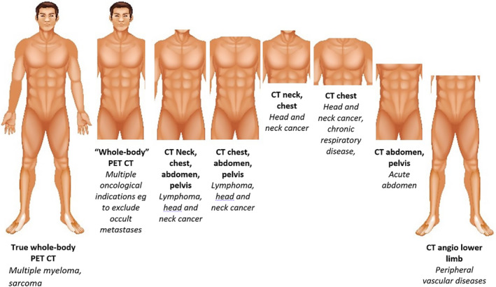
Common CT regional slabs in clinical practice. The variation in commonly CT scan regions is summarized. An opportunity to validate regional CT‐derived BC may be present in myeloma and sarcoma cohorts who have a true head‐to‐fingertip‐to‐toe CT. With the exception of true whole‐body PET CT, patients are scanned with arms up by default with the exception of critically ill or non‐compliant patients, as well as head and neck pathology or those with limited shoulder mobility.

It is not yet known how representative of the true whole body a regional volumetric slab is. Further research is required to validate the use of volumetric BC measures from common anatomical CT regions to estimate true head‐to‐toe volumes and to compare accuracy to single lumbar slice surface areas. This ultimately could be achieved with regression modelling in a similar manner to the landmark study validating the single lumbar slice technique, ¹⁹ with true whole‐body PET‐CT used in multiple myeloma as a potential source of scans with true head‐to‐toe coverage. ⁶⁹ However, a 2022 paper published after completion of this literature search makes progress towards this question. The authors trained a DL‐model to segment volumetric BC from a ‘whole body’ PET CT. The nomenclature is again confusing because the scans actually extended from head to mid‐thigh, missing the upper limbs and most of the lower limbs. However, they showed that the BC measures derived from the extended‐body PET CT were more strongly predicted by thoracic volumes compared with L3 surface area. ⁷⁰

Further research should also aim to determine which reproducible regions within a clinical CT slab most accurately predicts whole‐body BC. For example, a CT abdomen and pelvis will vary in start and end position between patients, and thus, it would be crucial to standardize the region to be segmented using fixed landmarks such as vertebral levels. To complicate things further, there is also variation in whether the upper limb is included in regional scans. With the exception of true whole‐body PET, the default position is having arms raised to lower radiation exposure, but patients with head and neck pathology, non‐compliant patients, critically ill patients and those with musculoskeletal conditions inhibiting shoulder abduction may have arms down. Future segmentation algorithms will need to have functionality to either include or exclude the upper limb from regional BC measures.

New cut‐offs for volumetric body composition measures

If regional volumetric CT slabs are shown to be a more accurate means of true BC estimation, a further challenge will lie in setting cut‐offs for CT‐defined sarcopenia and visceral obesity. This controversy presently exists for single slice analysis, where the SMI and body fat index are commonly used to standardize single‐slice surface area measurements by height and weight, respectively. There is a considerable heterogeneity in how studies set SMI cut‐offs for sarcopenia ⁷¹ including optimal stratification compared with a specific outcome such as overall survival ¹¹ , ²⁰ ; percentiles ⁷² ; standard deviations ⁷³ , ⁷⁴ ; or using ranges defined in previous studies. ⁷⁵ , ⁷⁶

New volume‐based metrics and cut‐offs will need to be determined for the various common clinical CT slabs. The only study from our review to address this problem was Lee et al., who calculated a cut ‐off for the average volumetric waist SMI that had high agreement with a clinical diagnosis of sarcopenia. ⁴³ Similar approaches should be explored in future studies.

Conclusions

This first systematic review of automated CT‐based volumetric BC analysis demonstrates speed, accuracy and feasibility of DL‐segmentation models. However, barriers and pitfalls are highlighted. Ground‐truth labelling standards require consensus definition. To avoid overfitting, DL models should be trained with as large a dataset as feasible, along with data augmentation. Metrics evaluating performance should quantify degree and direction of BC misclassification, in addition to DSC. External testing is crucial to ensure algorithms handle real‐world CT heterogeneity. These problems could be tackled by an international common dataset of prelabelled scans. This would also generate competition, leading to an optimal DL‐driven segmentation model. Evaluating segmentation precision, crucial for individualized longitudinal BC analysis, will likely require cadaveric or phantom studies due to unacceptability of CT test/retest in living patients.

Compared with single‐slice, additional computing power is required for volumetric segmentation and increased manpower for manual checks. Thus, it remains to be proven whether BC volumes from regional CT slabs more accurately measure total BC compared to single‐slice surface areas, and if this improved performance is sufficiently meaningful to justify costs. Furthermore, new volumetric SM and AT metrics and cut‐offs will need defining.

Conflict of interest

Dinh V C Mai, Ioanna Drami, Edward T Pring, Laura E Gould, Thanos Athanasiou and John T Jenkins have no conflicts of interest to declare. Karteek Popuri, Vincent Chow and Mirza F Beg are founding members of Voronoi Health Analytics Incorporated, a Canadian corporation selling commercial licences for the Data Analysis Facility Suite software. This software, capable of automated volumetric BC analysis from CT, is described in a study included in this systematic review. ⁴¹

Mai D. V. C., Drami I., Pring E. T., Gould L. E., Lung P., Popuri K., et al (2023) A systematic review of automated segmentation of 3D computed‐tomography scans for volumetric body composition analysis, Journal of Cachexia, Sarcopenia and Muscle, 14, 1973–1986, 10.1002/jcsm.13310

References

- 1. Au PCM, Li HL, Lee GKY, Li GH, Chan M, Cheung BM, et al. Sarcopenia and mortality in cancer: a meta‐analysis. Osteoporos Sarcopenia 2021;7:S28–S33. [DOI] [PMC free article] [PubMed] [Google Scholar]
- 2. Simonsen C, De Heer P, Bjerre ED, Suetta C, Hojman P, Pedersen BK, et al. Sarcopenia and postoperative complication risk in gastrointestinal surgical oncology. Ann Surg 2018;268:58–69. [DOI] [PubMed] [Google Scholar]
- 3. Yang M, Shen Y, Tan L, Li W. Prognostic value of sarcopenia in lung cancer: a systematic review and meta‐analysis. Chest 2019;156:101–111. [DOI] [PubMed] [Google Scholar]
- 4. Hua X, Liu S, Liao JF, Wen W, Long ZQ, Lu ZJ, et al. When the loss costs too much: a systematic review and meta‐analysis of sarcopenia in head and neck cancer. Front Oncol 2020;9:1561. [DOI] [PMC free article] [PubMed] [Google Scholar]
- 5. Zhang XM, Dou QL, Zeng Y, Yang Y, Cheng ASK, Zhang WW. Sarcopenia as a predictor of mortality in women with breast cancer: a meta‐analysis and systematic review. BMC Cancer 2020;20:1–11. [DOI] [PMC free article] [PubMed] [Google Scholar]
- 6. Fang P, Zhou J, Xiao X, Yang Y, Luan S, Liang Z, et al. The prognostic value of sarcopenia in oesophageal cancer: a systematic review and meta‐analysis. J Cachexia Sarcopenia Muscle 2023;14:3–16. [DOI] [PMC free article] [PubMed] [Google Scholar]
- 7. Guo Y, Ren Y, Zhu L, Yang L, Zheng C. Association between sarcopenia and clinical outcomes in patients with hepatocellular carcinoma: an updated meta‐analysis. Scientific Reports 2023;13:1–10. [DOI] [PMC free article] [PubMed] [Google Scholar]
- 8. Allanson ER, Peng Y, Choi A, Hayes S, Janda M, Obermair A. A systematic review and meta‐analysis of sarcopenia as a prognostic factor in gynecological malignancy. Int J Gynecol Cancer 2020;30:1791–1797. [DOI] [PubMed] [Google Scholar]
- 9. Trejo‐Avila M, Bozada‐Gutiérrez K, Valenzuela‐Salazar C, Herrera‐Esquivel J, Moreno‐Portillo M. Sarcopenia predicts worse postoperative outcomes and decreased survival rates in patients with colorectal cancer: a systematic review and meta‐analysis. Int J Colorectal Dis 2021;36:1077–1096. [DOI] [PubMed] [Google Scholar]
- 10. Caan BJ, Feliciano EMC, Prado CM, Alexeeff S, Kroenke CH, Bradshaw P, et al. Association of muscle and adiposity measured by computed tomography with survival in patients with nonmetastatic breast cancer. JAMA Oncol 2018;4:798. [DOI] [PMC free article] [PubMed] [Google Scholar]
- 11. Martin L, Birdsell L, Macdonald N, Clandinin MT, McCargar LJ, Murphy R, et al. Cancer cachexia in the age of obesity: skeletal muscle depletion is a powerful prognostic factor, independent of body mass index. J Clin Oncol 2013;31:1539–1547. [DOI] [PubMed] [Google Scholar]
- 12. Suetens P, Bellon E, Vandermeulen D, Smet M, Marchal G, Nuyts J, et al. Image segmentation: methods and applications in diagnostic radiology and nuclear medicine. Eur J Radiol 1993;17:14–21. [DOI] [PubMed] [Google Scholar]
- 13. Cespedes Feliciano EM, Popuri K, Cobzas D, Baracos VE, Beg MF, Khan AD, et al. Evaluation of automated computed tomography segmentation to assess body composition and mortality associations in cancer patients. J Cachexia Sarcopenia Muscle 2020;11:1258–1269. [DOI] [PMC free article] [PubMed] [Google Scholar]
- 14. Heymsfield SB, Wang ZM, Baumgartner RN, Ross R. Human body composition: advances in models and methods. Annu Rev Nutr 2003;17:527–558. [DOI] [PubMed] [Google Scholar]
- 15. Kvist H, Sjostrom L, Tylen U. Adipose tissue volume determinations in women by computed tomography: technical considerations. Int J Obes (Lond) 1986;10:53–67. Accessed August 16, 2022, https://europepmc.org/article/med/3710689 [PubMed] [Google Scholar]
- 16. Fowler PA, Fuller MF, Glasbey CA, Foster MA, Cameron GG, McNeill G, et al. Total and subcutaneous adipose tissue in women: the measurement of distribution and accurate prediction of quantity by using magnetic resonance imaging. Am J Clin Nutr 1991;54:18–25. [DOI] [PubMed] [Google Scholar]
- 17. Mitsiopoulos N, Baumgartner RN, Heymsfield SB, Lyons W, Gallagher D, Ross R. Cadaver validation of skeletal muscle measurement by magnetic resonance imaging and computerized tomography. J Appl Physiol 1998;85:115–122. [DOI] [PubMed] [Google Scholar]
- 18. Shen W, Chen J, Gantz M, Velasquez G, Punyanitya M, Heymsfield SB. A single MRI slice does not accurately predict visceral and subcutaneous adipose tissue changes during weight loss. Obesity 2012;20:2458–2463. [DOI] [PMC free article] [PubMed] [Google Scholar]
- 19. Shen W, Punyanitya M, Wang ZM, Gallagher D, St‐Onge MP, Albu J, et al. Total body skeletal muscle and adipose tissue volumes: estimation from a single abdominal cross‐sectional image. J Appl Physiol (1985) 2004;97:2333–2338. [DOI] [PubMed] [Google Scholar]
- 20. Prado CM, Lieffers JR, McCargar LJ, Reiman T, Sawyer MB, Martin L, et al. Prevalence and clinical implications of sarcopenic obesity in patients with solid tumours of the respiratory and gastrointestinal tracts: a population‐based study. Lancet Oncol 2008;9:629–635. [DOI] [PubMed] [Google Scholar]
- 21. Malietzis G, Currie AC, Athanasiou T, Johns N, Anyamene N, Glynne‐Jones R, et al. Influence of body composition profile on outcomes following colorectal cancer surgery. 2016;103:572–580. [DOI] [PubMed] [Google Scholar]
- 22. Prado CMM, Baracos VE, McCargar LJ, Reiman T, Mourtzakis M, Tonkin K, et al. Sarcopenia as a determinant of chemotherapy toxicity and time to tumor progression in metastatic breast cancer patients receiving capecitabine treatment. Clin Cancer Res 2009;15:2920–2926. [DOI] [PubMed] [Google Scholar]
- 23. Malietzis G, Currie AC, Johns N, Fearon KC, Darzi A, Kennedy RH, et al. Skeletal muscle changes after elective colorectal cancer resection: a longitudinal study. Ann Surg Oncol 2016;23:2539. [DOI] [PMC free article] [PubMed] [Google Scholar]
- 24. Mourtzakis M, Prado CM, Lieffers JR, Reiman T, McCargar LJ, Baracos VE. A practical and precise approach to quantification of body composition in cancer patients using computed tomography images acquired during routine care. Appl Physiol Nutr Metab 2008;33:997–1006. [DOI] [PubMed] [Google Scholar]
- 25. Linge J, Borga M, West J, Tuthill T, Miller MR, Dumitriu A, et al. Body composition profiling in the UK Biobank imaging study. Obesity (Silver Spring) 2018;26:1785–1795. [DOI] [PMC free article] [PubMed] [Google Scholar]
- 26. Karlsson A, Rosander J, Romu T, Tallberg J, Grönqvist A, Borga M, et al. Automatic and quantitative assessment of regional muscle volume by multi‐atlas segmentation using whole‐body water–fat MRI. J Magn Reson Imaging 2015;41:1558–1569. [DOI] [PubMed] [Google Scholar]
- 27. West J, Leinhard OD, Romu T, Collins R, Garratt S, Bell JD, et al. Feasibility of MR‐based body composition analysis in large scale population studies. PLoS ONE 2016;11. [DOI] [PMC free article] [PubMed] [Google Scholar]
- 28. Whitcher B, Thanaj M, Cule M, Liu Y, Basty N, Sorokin EP, et al. Precision MRI phenotyping enables detection of small changes in body composition for longitudinal cohorts. Scientific Reports 2022, 1;12:1–11. [DOI] [PMC free article] [PubMed] [Google Scholar]
- 29. Page MJ, McKenzie JE, Bossuyt PM, Boutron I, Hoffmann TC, Mulrow CD, et al. The PRISMA 2020 statement: an updated guideline for reporting systematic reviews. BMJ 2021:372. [DOI] [PMC free article] [PubMed] [Google Scholar]
- 30. Covidence systematic review software, Veritas Health Innovation, Melbourne, Australia. Available at www.covidence.org
- 31. Faes L, Liu X, Wagner SK, Fu DJ, Balaskas K, Sim DA, et al. A clinician's guide to artificial intelligence: how to critically appraise machine learning studies. Transl Vis Sci Technol 2020;9:7. [DOI] [PMC free article] [PubMed] [Google Scholar]
- 32. A Dictionary of Environment and Conservation. A dictionary of environment and conservation. Published online January 1, 2007.
- 33. Woodhouse IH. On ‘ground’ truth and why we should abandon the term. J Appl Remote Sens 2021;15:041501. [Google Scholar]
- 34. Brouwer NPM, Stijns RCH, Lemmens VEPP, Nagtegaal ID, B‐T RGH, Fütterer JJ, et al. Clinical lymph node staging in colorectal cancer; a flip of the coin? Eur J Surg Oncol 2018;44:1241–1246. [DOI] [PubMed] [Google Scholar]
- 35. Taha AA, Hanbury A. Metrics for evaluating 3D medical image segmentation: analysis, selection, and tool. BMC Med Imaging 2015;15:1–28. [DOI] [PMC free article] [PubMed] [Google Scholar]
- 36. Yeghiazaryan V, Voiculescu I. Family of boundary overlap metrics for the evaluation of medical image segmentation. J Med Imag 2018;5:1. [DOI] [PMC free article] [PubMed] [Google Scholar]
- 37. Hu P, Huo Y, Kong D, Carr JJ, Abramson RG, Hartley KG et al. Automated characterization of body composition and frailty with clinically acquired CT. Computational Methods and Clinical Applications in Musculoskeletal Imaging: 5th International Workshop, MSKI 2017, Held in Conjunction with MICCAI 2017, Quebec City, QC, Canada, September 10, 2017, Revised Selected Papers/Ben Glocker, Jianhua Yao, Toma 2018;10734:25‐35. [DOI] [PMC free article] [PubMed]
- 38. Decazes P, Tonnelet D, Vera P, Gardin I. Anthropometer3D: automatic multi‐slice segmentation software for the measurement of anthropometric parameters from CT of PET/CT. J Digit Imaging 2019;32:241–250. [DOI] [PMC free article] [PubMed] [Google Scholar]
- 39. Fu Y, Ippolito JE, Ludwig DR, Nizamuddin R, Li HH, Yang D. Technical note: automatic segmentation of CT images for ventral body composition analysis. Med Phys 2020;47:5723–5730. [DOI] [PubMed] [Google Scholar]
- 40. Liu T, Pan J, Torigian DA, Xu P, Miao Q, Tong Y, et al. ABCNet: A new efficient 3D dense‐structure network for segmentation and analysis of body tissue composition on body‐torso‐wide CT images. Med Phys 2020;47:2986–2999. [DOI] [PubMed] [Google Scholar]
- 41. Ma Da, Chow Vincent, Popuri Karteek, Beg Mirza Faisal. Comprehensive validation of automated whole body skeletal muscle, adipose tissue, and bone segmentation from 3D CT images for body composition analysis: towards extended body composition. ArXiv. 2021;Preprint.
- 42. Koitka S, Kroll L, Malamutmann E, Oezcelik A, Nensa F. Fully‐automated body composition analysis in routine CT imaging using 3D semantic segmentation convolutional neural networks. ArXiv 2021. [DOI] [PMC free article] [PubMed]
- 43. Lee YS, Hong N, Witanto JN, Choi YR, Park J, Decazes P, et al. Deep neural network for automatic volumetric segmentation of whole‐body CT images for body composition assessment. Clin Nutr 2021;40:5038–5046. [DOI] [PubMed] [Google Scholar]
- 44. Ma D, Chow V, Popuri K, Faisal Beg M. Comprehensive validation of automated whole body skeletal muscle, adipose tissue, and bone segmentation from 3D CT images for body composition analysis: towards extended body composition.
- 45. Wang M, Li P. Label fusion method combining pixel greyscale probability for brain MR segmentation. Scientific Reports 2019;9:1–10. [DOI] [PMC free article] [PubMed] [Google Scholar]
- 46. Ding W, Li L, Zhuang X, Huang L. Cross‐modality multi‐atlas segmentation using deep neural networks. Published online August 14, 2020.
- 47. Hong N, Kim KJ, Lee SJ, Kim CO, Kim HC, Rhee Y, et al. Cohort profile: Korean Urban Rural Elderly (KURE) study, a prospective cohort on ageing and health in Korea. BMJ Open 2019;9:e031018. [DOI] [PMC free article] [PubMed] [Google Scholar]
- 48. Chen LK, Woo J, Assantachai P, Auyeung TW, Chou MY, Iijima K, et al. Asian Working Group for Sarcopenia: 2019 Consensus Update on Sarcopenia Diagnosis and Treatment. J Am Med Dir Assoc 2020;21:300–307.e2. [DOI] [PubMed] [Google Scholar]
- 49. Higgins MI, Marquardt JP, Master VA, Fintelmann FJ, Psutka SP. Machine learning in body composition analysis. Eur Urol Focus 2021;7:713–716. [DOI] [PubMed] [Google Scholar]
- 50. Wang B, Torriani M. Artificial Intelligence in the evaluation of body composition. Semin Musculoskelet Radiol 2020;24:30–37. [DOI] [PubMed] [Google Scholar]
- 51. Bates DDB, Pickhardt PJ. CT‐derived body composition assessment as a prognostic tool in oncologic patients: from opportunistic research to artificial intelligence‐based clinical implementation. AJR Am J Roentgenol 2022;219:671–680. [DOI] [PubMed] [Google Scholar]
- 52. Greco F, Mallio CA. Artificial intelligence and abdominal adipose tissue analysis: a literature review. Quant Imaging Med Surg 2021;11:4461. [DOI] [PMC free article] [PubMed] [Google Scholar]
- 53. Stallings WM, Gillmore GM. A note on ‘accuracy’ and ‘precision’. J Educ Meas 1971;8:127–129. [Google Scholar]
- 54. Tabusa H, Blazeby JM, Blencowe N, Callaway M, Daniels IR, Gunning A, et al. Protocol for the UK cohort study to investigate the prevention of parastomal hernia (the CIPHER study). Colorectal Dis 2021;23:1900–1908. [DOI] [PubMed] [Google Scholar]
- 55. Arribas L, Sabaté‐Llobera A, Domingo MC, Taberna M, Sospedra M, Martin L, et al. Assessing dynamic change in muscle during treatment of patients with cancer: precision testing standards. Clin Nutr 2022;41:1059–1065. [DOI] [PubMed] [Google Scholar]
- 56. Hangartner TN, Warner S, Braillon P, Jankowski L, Shepherd J. The Official Positions of the International Society for Clinical Densitometry: acquisition of dual‐energy X‐ray absorptiometry body composition and considerations regarding analysis and repeatability of measures. J Clin Densitom 2013;16:520–536. [DOI] [PubMed] [Google Scholar]
- 57. Alavi DH, Sakinis T, Berg Henriksen H, Beichmann B, Fløtten A‐M, Blomhoff R, et al. Body composition assessment by artificial intelligence from routine computed tomography scans in colorectal cancer: Introducing BodySegAI. JCSM Clin Rep 2022;7:55–64. [Google Scholar]
- 58. Warfield SK, Zou KH, Wells WM. Simultaneous Truth and Performance Level Estimation (STAPLE): an algorithm for the validation of image segmentation. IEEE Trans Med Imaging 2004;23:903. [DOI] [PMC free article] [PubMed] [Google Scholar]
- 59. Winzeck S, Hakim A, McKinley R, Pinto JAADSR, Alves V, Silva C, et al. ISLES 2016 and 2017‐benchmarking ischemic stroke lesion outcome prediction based on multispectral MRI. Front Neurol 2018;9:679. [DOI] [PMC free article] [PubMed] [Google Scholar]
- 60. Commowick O, Istace A, Kain M, Laurent B, Leray F, Simon M, et al. Objective evaluation of multiple sclerosis lesion segmentation using a data management and processing infrastructure. Sci Rep 2018;8:13650. [DOI] [PMC free article] [PubMed] [Google Scholar]
- 61. Qiu Y, Hu Y, Kong P, Xie H, Zhang X, Cao J, et al. Automatic prostate gleason grading using pyramid semantic parsing network in digital histopathology. Front Oncol 2022;12:772403. [DOI] [PMC free article] [PubMed] [Google Scholar]
- 62. Nai YH, Teo BW, Tan NL, O'Doherty S, Stephenson MC, Thian YL, et al. Comparison of metrics for the evaluation of medical segmentations using prostate MRI dataset. Comput Biol Med 2021;134:104497. [DOI] [PubMed] [Google Scholar]
- 63. Diessel E, Fuerst T, Njeh CF, Tylavsky F, Cauley J, Dockrell M, et al. Evaluation of a new body composition phantom for quality control and cross‐calibration of DXA devices. J Appl Physiol 2000;89:599–605. [DOI] [PubMed] [Google Scholar]
- 64. Collins GS, Reitsma JB, Altman DG, Moons KGM. Transparent reporting of a multivariable prediction model for individual prognosis or diagnosis (TRIPOD): the TRIPOD statement. BMC Med 2015;13:1–10. [DOI] [PMC free article] [PubMed] [Google Scholar]
- 65. Liu X, Faes L, Kale AU, Wagner SK, Fu DJ, Bruynseels A, et al. A comparison of deep learning performance against health‐care professionals in detecting diseases from medical imaging: a systematic review and meta‐analysis. Articles Lancet Digital Health 2019;1:271–297. [DOI] [PubMed] [Google Scholar]
- 66. Rister B, Yi D, Shivakumar K, Nobashi T, Rubin DL. CT‐ORG, a new dataset for multiple organ segmentation in computed tomography. Scientific Data 2020;7:1–9. [DOI] [PMC free article] [PubMed] [Google Scholar]
- 67. Setio AAA, Traverso A, de Bel T, Berens MSN, Bogaard CVD, Cerello P, et al. Validation, comparison, and combination of algorithms for automatic detection of pulmonary nodules in computed tomography images: the LUNA16 challenge. Med Image Anal 2017;42:1–13. [DOI] [PubMed] [Google Scholar]
- 68. Bilic P, Christ P, Li HB, Vorontsov E, Ben‐Cohen A, Kaissis G, et al. The Liver Tumor Segmentation Benchmark (LiTS). Med Image Anal 2023;84:102680. [DOI] [PMC free article] [PubMed] [Google Scholar]
- 69. Mesguich C, Hulin C, Latrabe V, Lascaux A, Bordenave L, Hindié E. 18F‐FDG PET/CT and MRI in the management of multiple myeloma: a comparative review. Front Nucl Med 2022;12. [Google Scholar]
- 70. Pu L, Ashraf SF, Gezer NS, Ocak I, Dresser DE, Leader JK, et al. Estimating 3‐D whole‐body composition from a chest CT scan. Med Phys 2022;49:7108–7117. [DOI] [PMC free article] [PubMed] [Google Scholar]
- 71. Walowski CO, Braun W, Maisch MJ, Jensen B, Peine S, Norman K, et al. Reference values for skeletal muscle mass‐current concepts and methodological considerations. Nutrients 12:755. [DOI] [PMC free article] [PubMed] [Google Scholar]
- 72. van der Werf A, Langius JAE, de van der Schueren MAE, Nurmohamed SA, van der Pant KAMI, Blauwhoff‐Buskermolen S, et al. Percentiles for skeletal muscle index, area and radiation attenuation based on computed tomography imaging in a healthy Caucasian population. Eur J Clin Nutr 2018;72:288. [DOI] [PMC free article] [PubMed] [Google Scholar]
- 73. Derstine BA, Holcombe SA, Ross BE, Wang NC, Su GL, Wang SC. Optimal body size adjustment of L3 CT skeletal muscle area for sarcopenia assessment. Scientific Reports 2021;11:1–10. [DOI] [PMC free article] [PubMed] [Google Scholar]
- 74. Kim JS, Kim WY, Park HK, Kim MC, Jung W, Ko BS. Simple age specific cutoff value for sarcopenia evaluated by computed tomography. Ann Nutr Metab 2017;71:157–163. [DOI] [PubMed] [Google Scholar]
- 75. Nishigori T, Tsunoda S, Okabe H, Tanaka E, Hisamori S, Hosogi H, et al. Impact of sarcopenic obesity on surgical site infection after laparoscopic total gastrectomy. Ann Surg Oncol 2016;23:524–531. [DOI] [PubMed] [Google Scholar]
- 76. Pecorelli N, Carrara G, de Cobelli F, Cristel G, Damascelli A, Balzano G, et al. Effect of sarcopenia and visceral obesity on mortality and pancreatic fistula following pancreatic cancer surgery. Br J Surg 2016;103:434–442. [DOI] [PubMed] [Google Scholar]