Explainable machine learning model for predicting skeletal muscle loss during surgery and adjuvant chemotherapy in ovarian cancer

Abstract

Background

Skeletal muscle loss during treatment is associated with poor survival outcomes in patients with ovarian cancer. Although changes in muscle mass can be assessed on computed tomography (CT) scans, this labour‐intensive process can impair its utility in clinical practice. This study aimed to develop a machine learning (ML) model to predict muscle loss based on clinical data and to interpret the ML model by applying SHapley Additive exPlanations (SHAP) method.

Methods

This study included the data of 617 patients with ovarian cancer who underwent primary debulking surgery and platinum‐based chemotherapy at a tertiary centre between 2010 and 2019. The cohort data were split into training and test sets based on the treatment time. External validation was performed using 140 patients from a different tertiary centre. The skeletal muscle index (SMI) was measured from pre‐ and post‐treatment CT scans, and a decrease in SMI ≥ 5% was defined as muscle loss. We evaluated five ML models to predict muscle loss, and their performance was determined using the area under the receiver operating characteristic curve (AUC) and F1 score. The features for analysis included demographic and disease‐specific characteristics and relative changes in body mass index (BMI), albumin, neutrophil‐to‐lymphocyte ratio (NLR), and platelet‐to‐lymphocyte ratio (PLR). The SHAP method was applied to determine the importance of the features and interpret the ML models.

Results

The median (inter‐quartile range) age of the cohort was 52 (46–59) years. After treatment, 204 patients (33.1%) experienced muscle loss in the training and test datasets, while 44 (31.4%) patients experienced muscle loss in the external validation dataset. Among the five evaluated ML models, the random forest model achieved the highest AUC (0.856, 95% confidence interval: 0.854–0.859) and F1 score (0.726, 95% confidence interval: 0.722–0.730). In the external validation, the random forest model outperformed all ML models with an AUC of 0.874 and an F1 score of 0.741. The results of the SHAP method showed that the albumin change, BMI change, malignant ascites, NLR change, and PLR change were the most important factors in muscle loss. At the patient level, SHAP force plots demonstrated insightful interpretation of our random forest model to predict muscle loss.

Conclusions

Explainable ML model was developed using clinical data to identify patients experiencing muscle loss after treatment and provide information of feature contribution. Using the SHAP method, clinicians may better understand the contributors to muscle loss and target interventions to counteract muscle loss.

Introduction

Ovarian cancer is the most lethal gynaecological malignancy, with approximately 313 959 new cases and 207 252 deaths worldwide in 2020. ¹ The treatment for ovarian cancer is cytoreductive surgery with adjuvant or neoadjuvant chemotherapy. However, skeletal muscle loss occurs during treatment and compromises the survival outcomes. ² , ³ , ⁴ , ⁵ , ⁶ , ⁷ Muscle loss can be overlooked and may not be identified by changes in body weight. ⁵ Therefore, muscles in these patients should be assessed to identify loss and target interventions to preserve and recover muscle.

Skeletal muscle mass can be objectively measured using cross‐sectional computed tomography (CT) at the level of the third lumbar vertebra (L3). ⁸ Previous studies have revealed the usefulness of CT‐based muscle measurements in patients with ovarian cancer. ³ , ⁴ , ⁵ , ⁶ However, the utility of such measurements may be limited in clinical practice because the required process is labour‐intensive and time‐consuming. ⁹ To assess changes in muscle, pre‐ and post‐treatment CT scans should be processed by specific software, and the muscle is manually or semi‐automatically segmented on a cross‐sectional image at L3 to calculate the area of skeletal muscle. The skeletal muscle index (SMI) is then calculated using the muscle area and patient height, and the changes in muscle mass are evaluated. ¹⁰ , ¹¹ , ¹² However, the CT scans at L3 may be unavailable for analysis. Therefore, simpler methods to identify patients with muscle loss in clinical practice should be devised.

Machine learning (ML) has recently demonstrated favourable performance in predicting clinical information, such as outcomes and diagnoses. Compared to traditional statistical methods, ML can handle complex interactions and non‐linear relationships, leading to its increased use in clinical research where the outcomes of interest often depend on complex relationships between many factors. ¹³ , ¹⁴ , ¹⁵ While ML has undergone significant and continuous progress in the past decade, ML models are often considered black boxes that are difficult to interpret. Recent advances in explainable artificial intelligence methods can help to interpret ML models. Explainable artificial intelligence is a set of methods that allows clinicians and researchers to comprehend the decision‐making processes and output created by ML algorithms. This approach has also been proposed to make ML models more transparent and thus help advance the adoption of artificial intelligence in clinical practice. ¹⁶ Therefore, we hypothesized that ML models may enable clinicians to predict muscle loss from clinical data, and using explainable artificial intelligence methods may enable clinicians to interpret the ML model predictions for a patient and provide deeper insights into muscle loss. ¹⁴

This study aimed to develop an explainable ML model using clinical data to predict skeletal muscle loss during treatment in patients with ovarian cancer and to assess the feasibility of explainable ML models in clinical practice.

Materials and methods

Study population

This retrospective cohort study examined ML models to predict skeletal muscle loss in patients with ovarian cancer. This study was approved by Institutional Review Board of MacKay Memorial Hospital (MMH) and Changhua Christian Hospital (CCH), and the requirement for informed consent was waived because the study met the criteria for minimal risk to the study participants. We followed the reporting guidelines in TRIPOD (transparent reporting of a multivariate prediction model for individual prognosis or diagnosis).

The dataset was obtained from the institutional gynaecological cancer database of MMH and CCH. The data from MMH were used to train and test ML models, whereas the data from CCH were used for external validation. We reviewed patients diagnosed with International Federation of Gynecology and Obstetrics (FIGO) stage IC–IVA ovarian cancer and treated with primary debulking surgery (PDS) and adjuvant platinum‐based chemotherapy at MMH between January 2010 and December 2019 and at CCH between January 2017 and December 2019. Patients were included in the analysis if they had CT scans within 2 weeks before PDS and within 3 months after adjuvant chemotherapy and blood tests within 1 week before each CT scan. We excluded patients with any of the following characteristics: (1) refusal to undergo chemotherapy, (2) no follow‐up data, (3) CT scans of insufficient quality, and (4) missing blood test data. From 937 screened patients from these two institutions, 757 patients were included in this study (Figure  S1 ).

Data processing

Feature selection was performed using domain expertise, and features with potential discriminative power to predict muscle loss were selected. ⁵ , ¹³ , ¹⁷ , ¹⁸ , ¹⁹ Demographic features included age, Eastern Cooperative Oncology Group (ECOG) performance status, and body mass index (BMI). Disease‐specific features included FIGO stage, histological type and grade, residual disease status after PDS, and malignant ascites. Systemic inflammatory features included serum albumin, neutrophil‐to‐lymphocyte ratio (NLR), and platelet‐to‐lymphocyte ratio (PLR). The relative changes (%) in BMI, albumin, NLR, and PLR were calculated based on the corresponding values at the times of pre‐ and post‐treatment CT scans. Changes in these features were selected for analysis because changes in BMI and systemic inflammation are dynamic and associated with muscle loss during treatment. ⁹ Using longitudinal data also provides more useful information than using values at a single timepoint in ovarian cancer. ⁶ The data for the included patients were complete because records with missing values were excluded, and the application of an imputation method was not required. For data standardization, features were rescaled with respect to the z scores.

Outcome variable

Skeletal muscle change was calculated using pre‐ and post‐treatment CT scans acquired before PDS and within 3 months of adjuvant chemotherapy completion, respectively. One researcher, who was blinded to the patient information, used the 3D Slicer software (Version 4.11) to measure the cross‐sectional area (cm²) of the skeletal muscle on a single axial CT image at L3. Hounsfield units between −29 and +150 were used to define skeletal muscle areas, ⁸ which were normalized based on the patient's height to determine the SMI (cm²/m²). The change (%) in SMI during treatment was calculated as

$$\mathit{SMI}\mathit{\text{change}}\left(\%\right)=\frac{{\mathit{SMI}}_{\mathit{\text{post}}-\mathit{\text{treatment}}}-{\mathit{SMI}}_{\mathit{pre}-\mathit{\text{treatment}}}}{{\mathit{SMI}}_{\mathit{pre}-\mathit{\text{treatment}}}}\times 100$$

According to the current definition of cachexia and our previous studies, a decrease in SMI of at least 5% is classified as muscle loss, while a decrease below 5% or gain of SMI is classified as muscle maintain. ⁵ , ²⁰

Machine learning models

We split the data from MMH into training and test sets based on the treatment time. Data from patients treated between January 2010 and December 2016 were selected for the training set to construct the models, while data from patients treated between January 2017 and December 2019 were used for the model internal testing. The data from CCH were used for external validation.

We constructed and tested five supervised ML models: logistic regression (LR), random forest (RF), k‐nearest neighbour (K‐NN), support vector machine (SVM), and extreme gradient boosting (XGBoost). The Python Scikit‐learn library (Version 1.0.1, https://github.com/scikit‐learn/scikit‐learn) was used to build the ML models: (1) LR (LogisticRegression), (2) RF (RandomForestClassifier), (3) K‐NN (KNeighborsClassifier), (4) SVM (SVC), and (5) XGBoost (XGBClassifier). ²¹ The training set was randomly split into two subsets for training (70%) and validation (30%). The bootstrap method was implemented with 500 replications to derive the confidence interval (CI) of the area under the receiver operating characteristic curve (AUC), sensitivity, specificity, precision, and F1 score. The AUC and F1 score were the major indices of the model performance comparison. ²² , ²³ The five ML models were implemented using their default hyperparameter settings in the Python Scikit‐learn library.

We used the SHapley Additive exPlanations (SHAP) method to interpret the ML models and determine the effects of features on predictions. The SHAP method is useful for interpreting ML models at the cohort or patient level. ²⁴ The SHAP values of each feature for all the patients were separately aggregated and averaged to investigate the importance of the features for prediction. The SHAP feature importance plot shows the global importance of each feature where a larger mean absolute SHAP value of a feature indicates higher importance of the feature for model prediction. The SHAP summary plot shows the effect of each feature on the prediction model. Each dot on the SHAP summary plot represents a SHAP value for a feature per patient, and the colour from red to blue represents the feature value from high to low. SHAP dependence plots were created to explain the influence of certain features on the model prediction. The SHAP method was implemented in Python using SHAP Version 0.40.0.

Statistical analyses

Continuous data are presented as mean and standard deviation or median and inter‐quartile range (IQR), and categorical data are presented as frequencies and percentages. The patient and tumour characteristics between groups were compared using the chi‐squared test for categorical variables and independent‐samples t test for continuous variables. Changes in body composition and inflammatory parameters were assessed using paired t tests. All analyses were conducted using Python Version 3.7.3 and IBM SPSS (Version 26.0; IBM, Armonk, NY, USA). Statistical significance was set at P < 0.05 (two‐sided).

Results

Basic characteristics

A total of 757 were included in this study. Comparing pre‐ and post‐treatment CT scans in the entire cohort, the SMI decreased by 1.7% (41.2 vs. 40.3 cm²/m²; 95% CI: −1.1 to −0.6; P < 0.001). The changes in SMI were not significantly different between two institutions (−1.8% vs. −1.7%; P = 0.89). Among the patients, 204 (33.1%) patients experienced muscle loss during treatment in the training and test datasets, while 44 (31.4%) patients experienced muscle loss during treatment in the external validation dataset. The median (IQR) duration of CT scans was not significantly different between the groups (Table  1 ).

Table 1.

Patient and tumour characteristics

Characteristics	Training and test sets (n = 617)			External validation set (n = 140)
	Muscle loss (n = 204)	Muscle maintain (n = 413)	P value	Muscle loss (n = 44)	Muscle maintain (n = 96)	P value
Demographic data
Age (years)	53 (46–59)	51 (45–58)	0.19	52 (48–57)	53 (46–61)	0.75
ECOG performance status 1	91 (44.6)	84 (20.3)	<0.001	18 (40.9)	21 (21.9)	0.02
Pre‐treatment BMI (kg/m2)	22.8 ± 3.9	22.1 ± 3.1	0.02	22.7 ± 3.0	22.2 ± 2.6	0.29
Post‐treatment BMI (kg/m2)	22.5 ± 3.9	22.6 ± 3.1	0.81	22.4 ± 2.8	22.4 ± 2.7	0.99
Change in BMI (%)	−1.2 ± 5.8	2.3 ± 3.9	<0.001	−1.2 ± 4.4	1.1 ± 3.4	<0.001
Disease‐specific data
FIGO stage III–IVA	131 (64.2)	209 (50.6)	0.001	31 (70.5)	49 (51.0)	0.03
Serous carcinoma	115 (56.4)	214 (51.8)	0.29	26 (59.1)	51 (53.1)	0.51
Histological grade			0.002			0.02
Grade 1	24 (11.8)	93 (22.5)		4 (9.1)	23 (24.0)
Grade 2	73 (35.8)	145 (35.1)		13 (29.5)	36 (37.5)
Grade 3	107 (52.5)	175 (42.4)		27 (61.4)	37 (38.5)
Residual disease after PDS			<0.001			0.03
No residual disease	96 (47.1)	293 (70.9)		24 (54.5)	68 (70.8)
Residual disease ≤1 cm	63 (30.9)	83 (20.1)		12 (27.3)	23 (24.0)
Residual disease >1 cm	45 (22.1)	37 (9.0)		8 (18.2)	5 (5.2)
Malignant ascites	135 (66.2)	125 (30.3)	<0.001	30 (68.2)	31 (32.3)	<0.001
Systemic inflammatory data
Albumin (g/L)
Pre‐treatment	38.8 ± 5.4	40.7 ± 5.0	<0.001	40.4 ± 2.9	41.1 ± 3.5	0.21
Post‐treatment	35.4 ± 6.4	41.6 ± 4.9	<0.001	36.6 ± 4.0	41.9 ± 2.9	<0.001
Change (%)	−8.7 ± 11.7	2.6 ± 9.6	<0.001	−9.3 ± 9.4	2.3 ± 7.5	<0.001
NLR
Pre‐treatment	4.6 ± 4.4	4.3 ± 4.2	0.54	4.8 ± 3.5	4.5 ± 3.5	0.63
Post‐treatment	5.1 ± 5.1	2.4 ± 1.5	<0.001	5.0 ± 2.7	3.1 ± 2.0	<0.001
Change (%)	48.7 ± 144.7	−21.0 ± 52.9	<0.001	36.6 ± 86.7	−10.1 ± 50.4	<0.001
PLR
Pre‐treatment	273.4 ± 194.1	260.0 ± 279.9	0.54	237.1 ± 127.5	267.0 ± 205.6	0.38
Post‐treatment	265.5 ± 185.4	164.8 ± 78.0	<0.001	223.0 ± 120.0	193.0 ± 119.8	0.17
Change (%)	21.6 ± 86.4	−15.8 ± 47.9	<0.001	18.3 ± 87.2	−9.1 ± 52.8	0.02
Duration between CT scans (days)	174 (167–187)	175 (164–186)	0.84	176 (166–184)	176 (169–184)	0.70

Note: Data are median (IQR), mean ± standard deviation, or number (%). Abbreviations: BMI, body mass index; CT, computed tomography; ECOG, Eastern Cooperative Oncology Group; FIGO, International Federation of Gynecology and Obstetrics; IQR, inter‐quartile range; NLR, neutrophil‐to‐lymphocyte ratio; PDS, primary debulking surgery; PLR, platelet‐to‐lymphocyte ratio.

The patient characteristics are summarized in Table 1 . The median (IQR) age of the entire cohort was 52 (46–59) years. The distribution of age, ECOG, and disease‐specific features did not significantly differ between the training and test sets and external validation set. Patients with ECOG 1, FIGO stage III–IVA, higher histological grade, residual disease, and malignant ascites were more likely to experience muscle loss during treatment. In addition, patients in the muscle loss group had a significantly decreased BMI during treatment compared with patients in the muscle maintain group. Patients with muscle loss had significantly decreased albumin levels and increased NLR and PLR during treatment compared with patients with muscle maintenance in the training and test sets and external validation set.

Model evaluation and interpretation

Of the ML models used to predict muscle loss in the training set, RF and SVM exhibited the highest AUC (RF: 0.856, 95% CI: 0.854–0.859; SVM: 0.856, 95% CI: 0.853–0.859) (Figure 1 A and Table 2 ). The F1 score was used to further compare the performances of the ML models because the F1 score measures the accuracy in imbalanced datasets and reflects a harmonic combination of precision and recall, where precision is the positive predictive value and recall is the sensitivity. ²² , ²³ The RF model achieved the highest F1 score (0.726, 95% CI: 0.722–0.730). In the test set, the RF model also achieved a higher AUC value of 0.844 and F1 score of 0.706 (Figure 1 B and Table S1 ). With the independent external validation data (n = 140), the SVM and RF models exhibited higher AUC values (SVM: 0.880; RF: 0.874) among the five ML models (Figure 1 C ), while the RF model achieved the highest F1 score of 0.741 (Table  3 ). Therefore, downstream analysis was performed using the RF model.

Figure 1.

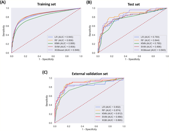
Receiver operating characteristic curves showing the muscle loss predictive performance of the machine learning models in (A, B) the training and test datasets and (C) external validation dataset. K‐NN, k‐nearest neighbour; LR, logistic regression; RF, random forest; SVM, support vector machine; XGBoost, extreme gradient boosting.

Table 2.

Evaluation of model performance in the training set

	AUC	Sensitivity	Specificity	Precision	F1 score
LR	0.845 (0.842, 0.848)	0.630 (0.624, 0.636)	0.921 (0.918, 0.923)	0.800 (0.794, 0.806)	0.702 (0.698, 0.707)
RF	0.856 (0.854, 0.859)	0.685 (0.679, 0.690)	0.903 (0.900, 0.906)	0.780 (0.775, 0.785)	0.726 (0.722, 0.730)
K‐NN	0.806 (0.803, 0.809)	0.579 (0.573, 0.585)	0.905 (0.903, 0.908)	0.754 (0.748, 0.760)	0.652 (0.648, 0.657)
SVM	0.856 (0.853, 0.859)	0.609 (0.604, 0.615)	0.929 (0.927, 0.932)	0.812 (0.807, 0.818)	0.694 (0.689, 0.698)
XGBoost	0.849 (0.846, 0.852)	0.682 (0.677, 0.688)	0.894 (0.891, 0.897)	0.764 (0.758, 0.770)	0.718 (0.714, 0.722)

Abbreviations: AUC, area under the receiver operating characteristic curve; K‐NN, k‐nearest neighbour; LR, logistic regression; RF, random forest; SVM, support vector machine; XGBoost, extreme gradient boosting.

Table 3.

Evaluation of the model performances in the external validation set

	AUC	Sensitivity	Specificity	Precision	F1 score
LR	0.832	0.704	0.854	0.688	0.696
RF	0.874	0.750	0.875	0.733	0.741
K‐NN	0.811	0.568	0.906	0.735	0.641
SVM	0.880	0.727	0.875	0.727	0.727
XGBoost	0.865	0.750	0.854	0.702	0.725

Abbreviations: AUC, area under the receiver operating characteristic curve; K‐NN, k‐nearest neighbour; LR, logistic regression; RF, random forest; SVM, support vector machine; XGBoost, extreme gradient boosting.

The SHAP feature importance for the RF model is shown in Figure 2 A . The evaluated features are ordered from the highest to lowest mean absolute SHAP values, ranking the impact of features on the prediction. The top 5 important features were the albumin change, BMI change, malignant ascites, NLR change, and PLR change. The SHAP summary plot of the RF model shows the impact of features on the prediction model (Figure 2 B ). Based on the prediction model, a higher SHAP value of a feature indicates a greater likelihood of muscle loss. For example, patients with decreased albumin levels during treatment are more likely to develop muscle loss compared to those with increased levels. In addition, patients with elevated NLR or PLR during treatment are more likely to develop muscle loss than those with decreased ratios. Furthermore, the SHAP dependence plot shows the effect of a feature on the RF prediction (Figure  3 ). Patients with decreased albumin levels and BMI (decrease in the x‐axis value) were associated with a higher SHAP value, indicating a higher likelihood of muscle loss (increase in the y‐axis value). Additionally, increased NLR and PLR values were associated with higher SHAP values.

Figure 2.

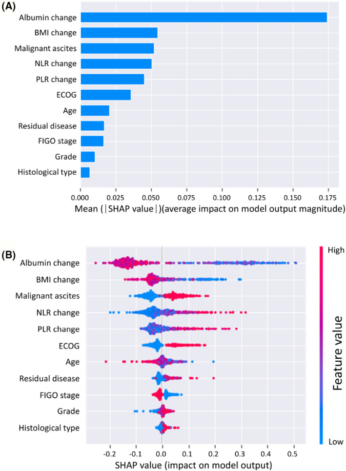
(A) SHapley Additive exPlanations (SHAP) feature importance shown according to the mean absolute SHAP value of each feature. (B) SHAP summary plot showing the distribution of the SHAP values of each feature. Each dot represents a SHAP value for a feature per patient. The x axis represents the SHAP value, and the colour varying from red to blue represents the feature value from high to low, respectively. BMI, body mass index; ECOG, Eastern Cooperative Oncology Group; FIGO, International Federation of Gynecology and Obstetrics; NLR, neutrophil‐to‐lymphocyte ratio; PLR, platelet‐to‐lymphocyte ratio.

Figure 3.

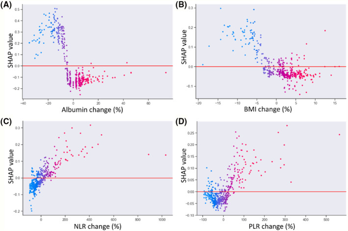
SHapley Additive exPlanations (SHAP) dependence plots of model features: (A) albumin change, (B) body mass index (BMI) change, (C) neutrophil‐to‐lymphocyte ratio (NLR) change, and (D) platelet‐to‐lymphocyte ratio (PLR) change. The y axis represents the SHAP values of features, and the values of certain features are shown in the x axis. Each dot represents a SHAP value for a feature per patient, and colour from red to blue represents the feature's value from high to low. SHAP values for specific features exceeding zero represent an increased risk of muscle loss development.

Explanation of machine learning model at the patient level

To evaluate the contributions of features for individual patients using the RF model, we applied the SHAP method to explain the individual predictions from two patients (Figure  4 ). The colour represents the contributions of each feature, with red being positive and blue being negative. The length of the colour bar represents the contribution strength. For Patient A, who was in the ‘true positive’ group, the RF model predicted a 92.0% probability of muscle loss (Figure 4 A ). For Patient B, who was in the ‘true negative’ group, the RF model predicted a 12.0% probability of muscle loss (Figure 4 B ).

Figure 4.

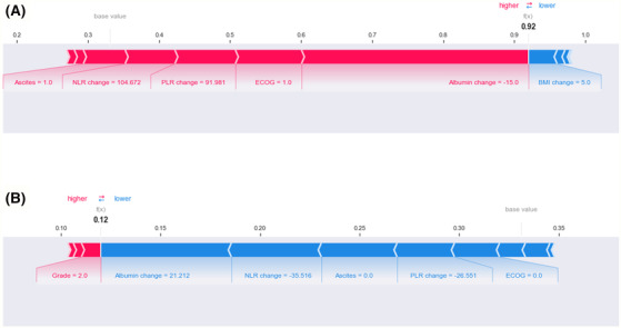
SHapley Additive exPlanations (SHAP) force plot of (A) Patient A (true positive) and (B) Patient B (true negative). The colour represents the contributions of each feature, with red being positive and blue being negative. The length of the colour bar represents the contribution strength. BMI, body mass index; ECOG, Eastern Cooperative Oncology Group; NLR, neutrophil‐to‐lymphocyte ratio; PLR, platelet‐to‐lymphocyte ratio.

Patient A was a 57‐year‐old woman with ECOG 1. She was diagnosed with FIGO stage III ovarian cancer, high‐grade serous carcinoma, and malignant ascites. The patient underwent complete resection with no macroscopic residual disease after PDS. Then, after adjuvant chemotherapy, the patient's SMI decreased by 6.3% and the BMI increased by 5.0%. She showed decreased albumin levels by 15% (40 vs. 34 g/L), increased NLR by 104.7% (1.6 vs. 3.2), and increased PLR by 92% (140.2 vs. 269.2). The results suggest that decreased albumin, ECOG 1, increased PLR and NLR, and the presence of malignant ascites are the main contributors to obtaining accurate muscle loss predictions.

Patient B was a 52‐year‐old woman with ECOG 0. The patient was diagnosed with FIGO stage III ovarian cancer with high‐grade serous carcinoma. Malignant ascites were not observed. The patient underwent complete resection with no macroscopic residual disease after PDS. After treatment, she exhibited an increased SMI by 17.5% and increased BMI by 4.1%. In terms of systemic inflammatory markers, she showed increased albumin levels by 21.2% (33 vs. 40 g/L), decreased NLR by 35.5% (3.6 vs. 2.3), and decreased PLR by 26.6% (197.8 vs. 145.3). The results suggest that increased albumin, decreased NLR, absence of malignant ascites, decreased PLR, and ECOG 0 are the main contributors of muscle maintenance.

Discussion

This is the first study to use ML models to predict muscle loss after PDS and adjuvant chemotherapy in patients with ovarian cancer. We evaluated five ML methods for prediction, with the RF model showing the highest performance. The RF model was also validated using external data from another hospital to ensure the credibility and generalizability of the results. Furthermore, we explored explanations of the RF model using the SHAP method. The most important features were the albumin change, BMI change, presence of malignant ascites, NLR change, and PLR change.

ML models for predicting CT‐based muscle loss in patients with oesophageal cancer have been evaluated in a previous study. ⁹ An ensemble model of LR and SVM using only changes in BMI and laboratory data as inputs achieved an AUC of 0.808. In addition to these data, we included other clinical and disease‐specific features to develop ML models, and the RF model achieved an AUC of 0.856 and F1 score of 0.726. In the external validation dataset, the RF model also outperformed the ML models with an AUC of 0.874 and F1 score of 0.741. To interpret our RF model, we identified the top predictors of muscle loss for the population using SHAP summary and dependence plots and for individual patients using SHAP force plots. The SHAP results showed that changes in BMI, albumin, NLR, and PLR, which can be easily evaluated in clinical practice, are important features for the ML model to predict muscle loss. In addition, the presence of malignant ascites is important in the RF model, suggesting catabolic effects of ascites on muscle mass in patients with ovarian cancer. ¹⁸

Systemic inflammation is a dynamic process, and its increase may trigger muscle breakdown. ¹⁷ Albumin has been recognized as a negative inflammatory marker related to systemic inflammation. The serum concentration of albumin decreases during the acute phase response associated with acute and chronic illness and inflammation. ²⁵ Conversely, NLR and PLR are positive inflammatory markers. ¹⁹ , ²⁶ Integrating serum albumin, NLR, and PLR in ML models may provide more comprehensive information regarding the patient's inflammatory state. ²⁷ Notably, the SHAP dependence plot shows the effect of inflammatory features on the RF prediction. In the two patients whose outcomes were correctly predicted, changes in these inflammatory features were the main contributors to the prediction, with additional contributions provided by the ECOG performance status and the presence of malignant ascites. Therefore, patients with muscle loss would likely present increased systemic inflammation after treatment, which triggers muscle breakdown. ¹⁷ These findings suggest that anti‐inflammatory interventions may modulate systemic inflammation to help preserve muscle during treatment for these patients. Nutrition and physical activity had been suggested to maintain muscle; however, the effectiveness of nutrition and physical activity can be limited in patients with increased systemic inflammation. ²⁸ , ²⁹ , ³⁰ Potential anti‐inflammatory interventions include eicosapentaenoic acid and some targeted anti‐inflammatory medications including anti‐interleukin‐6 (IL‐6) therapy or combined beta‐blocker and cyclooxygenase 2 inhibition. ³¹ , ³² , ³³ , ³⁴ , ³⁵ Exercise may also help reduce systemic inflammation and improve muscle in cancer patients. ³⁶ , ³⁷ However, whether these interventions based on the model predictions can modulate the inflammatory association of body composition with cancer outcomes remains unclear and needs to be investigated in future studies.

This study has various limitations. First, although our ML model was trained and tested using data from a single high‐volume gynaecological oncology centre and validated using a single external institution that is also a high‐volume gynaecological oncology centre, a more diverse population from multiple institutions is needed to further train and validate the ML model. Second, this study could not identify the timepoint at which patients experienced significantly lowered muscle mass during treatment because we could only analyse pre‐ and post‐treatment CT scans acquired during routine cancer care. In real‐world clinical practice, CT scans during treatment would be acquired only when clinically indicated. Therefore, in this study, CT scans for more diverse timepoints during surgery and adjuvant chemotherapy were unavailable for most patients. This study was also unable to identify whether surgery or chemotherapy was the major cause of muscle loss. Further studies with CT scans involving more timepoints may provide more comprehensive information to evaluate the prediction of muscle loss. Third, several variables were neglected in the models, including nutritional status, handgrip strength, physical activity, and other systemic inflammatory markers (e.g., C‐reactive protein and IL‐6), which may influence the model performance. Fourth, the ML model of this study may not be applicable to patients who undergo neoadjuvant chemotherapy and interval debulking surgery. PDS followed by adjuvant chemotherapy is the primary treatment for ovarian cancer, and all the patients in this study underwent such treatments. ³⁸ Neoadjuvant chemotherapy followed by interval debulking surgery is an alternative treatment option for ovarian cancer when PDS is not possible because of poor surgical candidates or a low likelihood of optimal cytoreduction. Although these two treatments have similar clinical outcomes, ³⁹ the differences in sequence of surgery and chemotherapy may contribute to different variations of muscle mass. Models for muscle loss predictions in patients who undergo neoadjuvant chemotherapy followed by interval debulking surgery need to be developed in future studies.

Conclusions

ML models using easily available clinical data can identify patients with muscle loss after PDS and adjuvant chemotherapy for ovarian cancer. The SHAP method allows the interpretation of predictions provided by ML models, leading to explainable ML models for clinical application. The explanations generated by the SHAP plots provide valuable insights into the sources of muscle loss for individual patients. This information may support patient counselling and targeted interventions to counteract muscle loss.

Funding information

This work was supported by the Ministry of Science and Technology, Taiwan (Contract Nos. MOST 110‐2314‐B‐195‐033 and MOST 110‐2314‐B‐A49A‐506‐MY3).

Conflict of interest statement

The authors declare no conflicts of interest.

Supporting information

Figure S1. Flow chart of the study design used to train, test, and externally validate the machine learning algorithms used to predict muscle loss in patients with ovarian cancer.

Table S1. Evaluation of model performance in the test set.

Hsu W.‐H., Ko A.‐T., Weng C.‐S., Chang C.‐L., Jan Y.‐T., Lin J.‐B., et al (2023) Explainable machine learning model for predicting skeletal muscle loss during surgery and adjuvant chemotherapy in ovarian cancer, Journal of Cachexia, Sarcopenia and Muscle, 14, 2044–2053, 10.1002/jcsm.13282

References

- 1. Sung H, Ferlay J, Siegel RL, Laversanne M, Soerjomataram I, Jemal A, et al. Global cancer statistics 2020: GLOBOCAN estimates of incidence and mortality worldwide for 36 cancers in 185 countries. CA Cancer J Clin 2021;71:209–249. [DOI] [PubMed] [Google Scholar]
- 2. Ubachs J, Ziemons J, Minis‐Rutten IJG, Kruitwagen R, Kleijnen J, Lambrechts S, et al. Sarcopenia and ovarian cancer survival: a systematic review and meta‐analysis. J Cachexia Sarcopenia Muscle 2019;10:1165–1174. [DOI] [PMC free article] [PubMed] [Google Scholar]
- 3. McSharry V, Glennon K, Mullee A, Brennan D. The impact of body composition on treatment in ovarian cancer: a current insight. Expert Rev Clin Pharmacol 2021;14:1065–1074. [DOI] [PubMed] [Google Scholar]
- 4. Polen‐de C, Fadadu P, Weaver AL, Moynagh M, Takahashi N, Jatoi A, et al. Quality is more important than quantity: pre‐operative sarcopenia is associated with poor survival in advanced ovarian cancer. Int J Gynecol Cancer 2022;32:1289–1296. [DOI] [PubMed] [Google Scholar]
- 5. Huang CY, Yang YC, Chen TC, Chen JR, Chen YJ, Wu MH, et al. Muscle loss during primary debulking surgery and chemotherapy predicts poor survival in advanced‐stage ovarian cancer. J Cachexia Sarcopenia Muscle 2020;11:534–546. [DOI] [PMC free article] [PubMed] [Google Scholar]
- 6. Rutten IJ, van Dijk DP, Kruitwagen RF, Beets‐Tan RG, Olde Damink SW, van Gorp T. Loss of skeletal muscle during neoadjuvant chemotherapy is related to decreased survival in ovarian cancer patients. J Cachexia Sarcopenia Muscle 2016;7:458–466. [DOI] [PMC free article] [PubMed] [Google Scholar]
- 7. Sutton EH, Plyta M, Fragkos K, Di Caro S. Pre‐treatment sarcopenic assessments as a prognostic factor for gynaecology cancer outcomes: systematic review and meta‐analysis. Eur J Clin Nutr 2022;76:1513–1527. [DOI] [PubMed] [Google Scholar]
- 8. Mourtzakis M, Prado CM, Lieffers JR, Reiman T, McCargar LJ, Baracos VE. A practical and precise approach to quantification of body composition in cancer patients using computed tomography images acquired during routine care. Appl Physiol Nutr Metab 2008;33:997–1006. [DOI] [PubMed] [Google Scholar]
- 9. Yoon HG, Oh D, Noh JM, Cho WK, Sun JM, Kim HK, et al. Machine learning model for predicting excessive muscle loss during neoadjuvant chemoradiotherapy in oesophageal cancer. J Cachexia Sarcopenia Muscle 2021;12:1144–1152. [DOI] [PMC free article] [PubMed] [Google Scholar]
- 10. Lee J, Chen TC, Jan YT, Li CJ, Chen YJ, Wu MH. Association of patient‐reported outcomes and nutrition with body composition in women with gynecologic cancer undergoing post‐operative pelvic radiotherapy: an observational study. Nutrients 2021;13:2629. [DOI] [PMC free article] [PubMed] [Google Scholar]
- 11. Lee J, Lin JB, Wu MH, Chang CL, Jan YT, Chen YJ. Muscle loss after chemoradiotherapy as a biomarker of distant failures in locally advanced cervical cancer. Cancers (Basel) 2020;12:595. [DOI] [PMC free article] [PubMed] [Google Scholar]
- 12. Lee J, Liu SH, Chen JC, Leu YS, Liu CJ, Chen YJ. Progressive muscle loss is an independent predictor for survival in locally advanced oral cavity cancer: a longitudinal study. Radiother Oncol 2021;158:83–89. [DOI] [PubMed] [Google Scholar]
- 13. Stevens LM, Mortazavi BJ, Deo RC, Curtis L, Kao DP. Recommendations for reporting machine learning analyses in clinical research. Circ Cardiovasc Qual Outcomes 2020;13:e006556. [DOI] [PMC free article] [PubMed] [Google Scholar]
- 14. Shi H, Yang D, Tang K, Hu C, Li L, Zhang L, et al. Explainable machine learning model for predicting the occurrence of postoperative malnutrition in children with congenital heart disease. Clin Nutr 2022;41:202–210. [DOI] [PubMed] [Google Scholar]
- 15. Chung H, Ko Y, Lee IS, Hur H, Huh J, Han SU, et al. Prognostic artificial intelligence model to predict 5 year survival at 1 year after gastric cancer surgery based on nutrition and body morphometry. J Cachexia Sarcopenia Muscle 2023;14:847–859. [DOI] [PMC free article] [PubMed] [Google Scholar]
- 16. Saeed W, Omlin C. Explainable AI (XAI): a systematic meta‐survey of current challenges and future opportunities. Knowl‐Based Syst 2023;263:110273. [Google Scholar]
- 17. Cole CL, Kleckner IR, Jatoi A, Schwarz EM, Dunne RF. The role of systemic inflammation in cancer‐associated muscle wasting and rationale for exercise as a therapeutic intervention. JCSM Clin Rep 2018;3:1–19. [PMC free article] [PubMed] [Google Scholar]
- 18. Ubachs J, van de Worp W, Vaes RDW, Pasmans K, Langen RC, Meex RCR, et al. Ovarian cancer ascites induces skeletal muscle wasting in vitro and reflects sarcopenia in patients. J Cachexia Sarcopenia Muscle 2022;13:311–324. [DOI] [PMC free article] [PubMed] [Google Scholar]
- 19. Zhang Q, Song MM, Zhang X, Ding JS, Ruan GT, Zhang XW, et al. Association of systemic inflammation with survival in patients with cancer cachexia: results from a multicentre cohort study. J Cachexia Sarcopenia Muscle 2021;12:1466–1476. [DOI] [PMC free article] [PubMed] [Google Scholar]
- 20. Fearon K, Strasser F, Anker SD, Bosaeus I, Bruera E, Fainsinger RL, et al. Definition and classification of cancer cachexia: an international consensus. Lancet Oncol 2011;12:489–495. [DOI] [PubMed] [Google Scholar]
- 21. Pedregosa F, Varoquaux G, Gramfort A, Michel V, Thirion B, Grisel O, et al. Scikit‐learn: machine learning in Python. J Mach Learn Res 2011;12:2825–2830. [Google Scholar]
- 22. Bekkar M, Djemaa HK, Alitouche TA. Evaluation measures for models assessment over imbalanced data sets. J Inf Eng Appl 2013;3:27–38. [Google Scholar]
- 23. Sokolova M, Lapalme G. A systematic analysis of performance measures for classification tasks. Inf Process Manag 2009;45:427–437. [Google Scholar]
- 24. Lundberg SM, Lee S‐I. A unified approach to interpreting model predictions. Adv Neural Inf Process Syst 2017;30:4765–4774. [Google Scholar]
- 25. Evans DC, Corkins MR, Malone A, Miller S, Mogensen KM, Guenter P, et al. The use of visceral proteins as nutrition markers: an ASPEN position paper. Nutr Clin Pract 2021;36:22–28. [DOI] [PubMed] [Google Scholar]
- 26. Ruan GT, Ge YZ, Xie HL, Hu CL, Zhang Q, Zhang X, et al. Association between systemic inflammation and malnutrition with survival in patients with cancer sarcopenia—a prospective multicenter study. Front Nutr 2022;8:811288. [DOI] [PMC free article] [PubMed] [Google Scholar]
- 27. Xie H, Ruan G, Wei L, Zhang H, Ge Y, Zhang Q, et al. Hand grip strength‐based cachexia index as a predictor of cancer cachexia and prognosis in patients with cancer. J Cachexia Sarcopenia Muscle 2023;14:382–390. [DOI] [PMC free article] [PubMed] [Google Scholar]
- 28. Merker M, Felder M, Gueissaz L, Bolliger R, Tribolet P, Kägi‐Braun N, et al. Association of baseline inflammation with effectiveness of nutritional support among patients with disease‐related malnutrition: a secondary analysis of a randomized clinical trial. JAMA Netw Open 2020;3:e200663. [DOI] [PMC free article] [PubMed] [Google Scholar]
- 29. Golder AM, Sin LKE, Alani F, Alasadi A, Dolan R, Mansouri D, et al. The relationship between the mode of presentation, CT‐derived body composition, systemic inflammatory grade and survival in colon cancer. J Cachexia Sarcopenia Muscle 2022;13:2863–2874. [DOI] [PMC free article] [PubMed] [Google Scholar]
- 30. Collao N, Sanders O, Caminiti T, Messeiller L, De Lisio M. Resistance and endurance exercise training improves muscle mass and the inflammatory/fibrotic transcriptome in a rhabdomyosarcoma model. J Cachexia Sarcopenia Muscle 2023;14:781–793. [DOI] [PMC free article] [PubMed] [Google Scholar]
- 31. Prado CM, Purcell SA, Laviano A. Nutrition interventions to treat low muscle mass in cancer. J Cachexia Sarcopenia Muscle 2020;11:366–380. [DOI] [PMC free article] [PubMed] [Google Scholar]
- 32. Fleming CA, O'Connell EP, Kavanagh RG, O'Leary DP, Twomey M, Corrigan MA, et al. Body composition, inflammation, and 5‐year outcomes in colon cancer. JAMA Netw Open 2021;4:e2115274. [DOI] [PMC free article] [PubMed] [Google Scholar]
- 33. Cornish SM, Cordingley DM, Shaw KA, Forbes SC, Leonhardt T, Bristol A, et al. Effects of omega‐3 supplementation alone and combined with resistance exercise on skeletal muscle in older adults: a systematic review and meta‐analysis. Nutrients 2022;14:2221. [DOI] [PMC free article] [PubMed] [Google Scholar]
- 34. Wu KC, Chu PC, Cheng YJ, Li CI, Tian J, Wu HY, et al. Development of a traditional Chinese medicine‐based agent for the treatment of cancer cachexia. J Cachexia Sarcopenia Muscle 2022;13:2073–2087. [DOI] [PMC free article] [PubMed] [Google Scholar]
- 35. Fan M, Gu X, Zhang W, Shen Q, Zhang R, Fang Q, et al. Atractylenolide I ameliorates cancer cachexia through inhibiting biogenesis of IL‐6 and tumour‐derived extracellular vesicles. J Cachexia Sarcopenia Muscle 2022;13:2724–2739. [DOI] [PMC free article] [PubMed] [Google Scholar]
- 36. Winker M, Stössel S, Neu MA, Lehmann N, El Malki K, Paret C, et al. Exercise reduces systemic immune inflammation index (SII) in childhood cancer patients. Support Care Cancer 2022;30:2905–2908. [DOI] [PMC free article] [PubMed] [Google Scholar]
- 37. Cao A, Cartmel B, Li FY, Gottlieb LT, Harrigan M, Ligibel JA, et al. Effect of exercise on body composition among women with ovarian cancer. J Cancer Surviv 2022. [DOI] [PMC free article] [PubMed] [Google Scholar]
- 38. National Comprehensive Cancer Network . Clinical practice guidelines in oncology: ovarian cancer [version 1.2023]. https://www.nccn.org/professionals/physician_gls/pdf/ovarian.pdf [DOI] [PubMed]
- 39. Fagotti A, Ferrandina MG, Vizzielli G, Pasciuto T, Fanfani F, Gallotta V, et al. Randomized trial of primary debulking surgery versus neoadjuvant chemotherapy for advanced epithelial ovarian cancer (SCORPION‐NCT01461850). Int J Gynecol Cancer 2020;30:1657–1664. [DOI] [PubMed] [Google Scholar]
- 40. von Haehling S, Morley JE, Coats AJS, Anker SD. Ethical guidelines for publishing in the Journal of Cachexia, Sarcopenia and Muscle: update 2021. J Cachexia Sarcopenia Muscle 2021;12:2259–2261. [DOI] [PMC free article] [PubMed] [Google Scholar]
Associated Data
This section collects any data citations, data availability statements, or supplementary materials included in this article.
Supplementary Materials