PERSISTENT PATH LAPLACIAN

Abstract

Path homology proposed by S.-T.Yau and his co-workers provides a new mathematical model for directed graphs and networks. Persistent path homology (PPH) extends the path homology with filtration to deal with asymmetry structures. However, PPH is constrained to purely topological persistence and cannot track the homotopic shape evolution of data during filtration. To overcome the limitation of PPH, persistent path Laplacian (PPL) is introduced to capture the shape evolution of data. PPL’s harmonic spectra fully recover PPH’s topological persistence and its non-harmonic spectra reveal the homotopic shape evolution of data during filtration.

1. Introduction.

Recent years witness the emergence of a variety of advanced mathematical tools in topological data analysis (TDA) [13]. As the main workhorse of TDA, persistent homology (PH) [2, 9, 43, 10] pioneered a new branch in algebraic topology, offering a powerful tool to decode the topological structures of data during filtration in terms of persistent Betti numbers. Persistent homology has had tremendous success in many areas of science and technology, such as biology [41], chemistry [35], drug discovery [29], 3D shape analysis [33], etc.

Inspired by the success of PH, other mathematical tools have been given due attention. One of them is de Rham-Hodge theory in differential geometry, which uses the differential forms to represent the cohomology of an oriented closed Riemannian manifold with boundary in terms of a topological Laplacian, namely Hodge Laplacian [8]. The de Rham-Hodge theory has been applied to computational biology [42], graphic [34], and robotics [28]. However, like homology, the de Rham-Hodge theory does not offer an in-depth analysis of data, which is a famous problem in spectral geometry [24]. To overcome this drawback, the evolutionary de Rham-Hodge theory [5] was introduced in terms of persistent Hodge Laplacian to offer a multiscale analysis of the de Rham-Hodge theory. Defined on a family of evolutionary manifolds, the evolutionary de Rham-Hodge theory gives a new answer to, or at least reopens, the famous 55-years old question “can one hear the shape of a drum”. [24] The persistent Hodge Laplacian captures both the topological persistence and the homotopic shape evolution of data during filtration.

Nevertheless, the evolutionary de Rham-Hodge theory is set up on Riemannian manifolds, which may be computationally demanding for large datasets. Hence, a similar multiscale-based topological Laplacian, called persistent spectral graph (PSG) [37], was proposed by introducing a filtration to combinatorial graph Laplacians. PSG, aka persistent Laplacian (PL) [26], extends persistent homology to non-harmonic analysis of data, showing much advantage in sophisticated applications [27, 4, 39]. Dealing with point cloud data instead of manifolds, PL encodes a point cloud to a family of simplicial complexes generated from filtration and analyzes both harmonic and non-harmonic spectra. It is worthy to notice that the harmonic spectra from the null spaces of PLs reveal the same topological persistence as that of persistent homology, whereas, the non-harmonic spectra of PLs capture the homotopic shape evolution of data during filtration. Meanwhile, open-source software called HERMES [38] was developed for the simultaneous topological and geometric analysis of data. However, like persistent homology, PSG treats all data points equally. That is to say, each point does not carry any labeled information such as the type, mass, color, etc. Therefore, an extension of PSG, called persistent sheaf Laplacian (PSL), was proposed to generalize cellular sheaves [32, 22] for the multiscale analysis of point cloud data with attached labeled information [40]. PSL is also a topological Laplacian that carries topological information in its null space but tracks homotopic shape evolution during filtration. It is worthy to mention that eigenvectors computed from Hodge Laplacians defined on manifolds [42] are sharply different from those computed from combinatorial Laplacians defined on simplicial complexes [39]. The minor similarity and fundamental difference of these Laplacians were discussed in the literature [31]. Another interesting development is the persistent Dirac Laplacian (PDL) by Ameneyro, Maroulas, and Siopsis [1]. PDL offers an efficient quantum computation of persistent Betti numbers across different scales. The above-mentioned approaches have great potentials to deal with complex data in science and engineering.

It is noticed that the aforementioned homologies and topological Laplacians are insensitive to asymmetry or directed relations, which limits their representational power in encoding structures that have directional information. For example, in gene regulation data, the directions of gene regulations are indicated by arrowheads or perpendicular edges in systems biology [25]. Therefore, a technique that can deal with directed graphs (digraphs) is of vital importance to inferring gene regulation relationships. Notably, the path homology [16] proposed by Grigor’yan, Lin, Muranov, and Yau provides a powerful tool to analyze datasets with asymmetric structures using the path complex. Particular cases of homologies of digraphs and their path cohomology were also discussed [16, 18, 20]. The notion of path homology of digraphs has a richer mathematical structure than the earlier homology and Laplacian, opening new directions for both pure and applied mathematics. For example, path homology theory was extended to various objects such as quivers, multigraphs, digraphs pairs, cylinder, cone, hypergraphs, etc. [21, 15, 14] Path homology has drawn much attention from researchers in the TDA community. To encode richer information, Chowdhury and Mémoli extended path homology to a persistent framework on a directed network [6]. Wang, Ren, and Wu constructed a weighted path homology for weight digraphs and proved a persistent version of a Künneth-type formula for joins of weighted digraphs [36]. Recently, Dey, Li, and Wang have designed an efficient algorithm for 1-dimensional persistent path homology [7], which is useful in real applications.

Similar to persistent homology, persistent path homology cannot track the homotopic shape evolution of data during filtration. To overcome this limitation, we introduce path Laplacian as a new topological Laplacian to analyze the spectral geometry of data, in addition to its topology. Moreover, we introduce a filtration to path Laplacian to obtain a persistent path Laplacian (PPL), a new framework that captures both the topological persistence and shape evolution of directed graphs and networks. By varying the filtration parameter, one can construct a series of digraphs, which result in a family of persistent path Laplacian matrices. The harmonic spectra of the persistent path Laplacian recover all the topological invariants of the digraphs, while the non-harmonic spectra provide additional geometric information, which can distinguish two systems when they are homotopy but geometrically different. PPL has potential applications in science, engineering, industry, and technology. This work is organized as follows: Section 2 reviews the necessary background on path homology. Section 3 describes path Laplacian and persistent path Laplacian. Detailed PPL matrix constructions are illustrated with various examples for the interested readers in Section 3 and Section 4.

2. Background on path homology and directed graph.

Graph structure offers a powerful and versatile data representation that encodes inter-dependencies among constituents, which has been driven by widely spread applications in various fields such as graph theory, topological data analysis, science, and engineering. In this section, we first recap basic concepts in path homology, including paths on a finite set, boundary operator on the path complex, and homologies of path complex. Then, we briefly review the concept of directed graphs (digraphs) and give a discussion of path homologies on the directed graph without self loops. Such concepts and notations, due to Yau and coworkers, form a basis for us to introduce path Laplacian and persistent path Laplacian in section 3.

2.1. Paths on a finite set.

Denote set $V$ an arbitrary nonempty finite set, and elements in $V$ are called vertices. For $p\in {\mathbb{Z}}_0^{+}$ (i.e., a set with integers $p\ge 0$), an elementary $p$-path on $V$ is any sequence $i_0\dots i_p$ of $p+1$ vertices in $V$. An elementary $p$-path is an empty set $\varnothing$ for $p=-1$. For a fixed field $\mathbb{K}$, a vector space that consists of all formal linear combinations of elementary $p$-paths with its coefficients in $\mathbb{K}$ is called the space generated by the elementary paths, denoted as ${\Lambda }_p={\Lambda }_p(V,\mathbb{K})={\Lambda }_p\left(V\right)$. One says the elements in ${\Lambda }_p$ are $p$-paths on $V$, and an elementary $p$-path $i_0\dots i_p\in {\Lambda }_p$ is denoted by $e_{i_0\dots i_p}$. By definition, $\forall v\in {\Lambda }_p$, its unique representation can be given by the basis in ${\Lambda }_p$:

$$v=\sum _{i_0,\dots ,i_p\in V}{c}^{i_0\dots i_p}{e}_{i_0\dots i_p},$$ (1)

where $c^{i_0\dots i_p}$ is the coefficient in $\mathbb{K}$. For instance, ${\Lambda }_0$ contains all linear combination of $e_i$ with $i\in V$, ${\Lambda }_1$ has all linear combination of $e_{ij}$ with $(i,j)\in V\times V$, and so on so forth. Since ${\Lambda }_{-1}$ consists of all multiples of $e$, one has ${\Lambda }_{-1}\cong \mathbb{K}$.

Additionally, $\forall p\in {\mathbb{Z}}_0^{+}$, the linear boundary operator from ${\Lambda }_p$ to ${\Lambda }_{p-1}$ that acts on elementary paths can be defined as

$$\partial :{\Lambda }_p\to {\Lambda }_{p-1}$$ (2)

with

$$\partial e_{i_0\dots i_p}=\sum _{q=0}^p{(-1)}^q{e}_{i_0\dots {\widehat{i}}_q\dots i_p},$$ (3)

where ${\hat{i}}_q$ denotes the omission of index $i_q$ from the elementary $p$-path $e_{i_0\dots i_p}$. One sets ${\Lambda }_{-2}=\left\{0\right\}$, and for $p=-1$, defines $\partial :{\Lambda }_{-1}\to {\Lambda }_{-2}$ to be a zero map. Following Lemma 2.1 in [19], one has ${\partial }^2=0$, which indicates that the collection of boundary operator $\partial$ and space ${\Lambda }_p$ can form a chain complex of $V$ denoted as ${\Lambda }_{*}=\left\{{\Lambda }_p\right\}$ as

$$\cdots {\Lambda }_p\stackrel{\partial }{\to }{\Lambda }_{p-1}\stackrel{\partial }{\to }\cdots \stackrel{\partial }{\to }{\Lambda }_0\stackrel{\partial }{\to }\mathbb{K}\stackrel{\partial }{\to }0.$$ (4)

Next, the concepts of regular path and non-regular path are introduced according to [19]. An elementary path $e_{i_0\dots i_p}$ on a set $V$ is regular if $i_{k-1}\ne i_k$, and non-regular if $i_{k-1}=i_k$ for $k=1,\dots ,p$. For any $p\in {\mathbb{Z}}_0^{+}\cup \{-1\}$, let ${ℛ}_p$ be the subspace of ${\Lambda }_p$ spanned by all regular elementary paths, and ${𝒩}_p$ be the subspace of ${\Lambda }_p$ spanned by all non-regular elementary paths. Therefore, one has

$${ℛ}_p=\text{span}\left\{e_{i_0\dots i_p}:i_0\dots i_p\text{\hspace{0.17em}is regular}\right\}$$

$${𝒩}_p=\text{span}\left\{e_{i_0\dots i_p}:i_0\dots i_p\text{\hspace{0.17em}is non-regular}\right\}.$$

Note that ${ℛ}_p={\Lambda }_p$ for integers $p=-\mathrm{1,0}$.

Then $\forall p\in {\mathbb{Z}}_0^{+}\cup \left\{-1\right\}$, ${\Lambda }_p={ℛ}_p\oplus {𝒩}_p$. Therefore,

$${ℛ}_p\cong {\Lambda }_p/{𝒩}_p$$

According to Section 2.4 in [19], the boundary operator $\partial$ is well-defined on the quotient space ${\Lambda }_p/{𝒩}_p$. Moreover, ${\partial }^2=0$ and the product rules are satisfied in the quotient space ${\Lambda }_p/{𝒩}_p$ as well. One has an induced regular boundary operator:

$$\overline{\partial }:{ℛ}_p\to {ℛ}_{p-1},$$ (5)

where the regular boundary operator $\bar{\partial }$ satisfies (3) except that all non-regular terms on the right hand side should be treated as 0. Then a chain complex of $V$, denoted as ${ℛ}_{*}\left(V\right)={\left({ℛ}_p\right)}_p$ and equipped with $\bar{\partial }$, can be expressed as:

$$\cdots {ℛ}_p\stackrel{\overline{\partial }}{\to }{ℛ}_{p-1}\stackrel{\overline{\partial }}{\to }\cdots \stackrel{\overline{\partial }}{\to }{ℛ}_0\stackrel{\overline{\partial }}{\to }\mathbb{K}\stackrel{\overline{\partial }}{\to }0.$$ (6)

It can be verified that $R_p\cong {\Lambda }_p/N_p$ is an isomorphism of chain complexes [18]. In the following sections, for simplicity, we use $\partial$ to denote the boundary operator of Eq. (6) unless specified differently.

2.2. Path complex.

A path complex over set $V$ is a nonempty collection $P$ of elementary paths on $V$ for any $n\in {\mathbb{Z}}_0^{+}$,

$$\text{if\hspace{0.17em}}{i}_0\dots i_n\in P,\text{ \hspace{0.17em}then\hspace{0.17em}}{i}_0\dots i_{n-1}\in P,\text{\hspace{0.17em} and\hspace{0.17em}}{i}_1\dots i_n\in P\text{.}$$ (7)

For a fixed path complex, all the paths from $P$ are called allowed (i.e. $i_{k-1}\to i_k$ for any $k=1,\dots ,n$), while the elementary paths on $V$ that are not in $P$ are non-allowed. We say a path complex $P$ is perfect if any subsequence of any path from $P$ is also in $P$. We choose $P_n$ to denote all $n$-paths from $P$. Then the set $P_{-1}$ has a single empty path $e$, the set $P_0$ consists of all the vertices of $P$, and clearly, $V=P_0$. To be noted, a path complex $P$ is a collection ${\left\{P_n\right\}}_{n=-1}^{\infty }$ satisfying Eq. (7). Let $𝒦$ be an abstract simplicial complex defined over a finite vertex set $V$, satisfying

$$\text{if }\sigma \in 𝒦,\text{ then any subset of }\sigma \text{ is also in }𝒦.$$

The collection of elementary paths on $V$ is denoted by $P\left(𝒦\right)$. Following Ref. [19] (cf. Example 3.2), the family $P\left(𝒦\right)$ is a path complex.

2.3. Path homology.

For any $n\in {\mathbb{Z}}_0^{+}$, the $\mathbb{K}$-linear space ${𝒜}_n$ is spanned by all the elementary $n$-paths from a given path complex $P={\left\{P_n\right\}}_{n=0}^{\infty }$ over a finite set $V$, i.e.,

$${𝒜}_n={𝒜}_n(P)=\text{span}\left\{e_{i_0\dots i_n}:i_0\dots i_n\in P_n\right\}.$$

We call the elements of ${𝒜}_n$ the allowed $n$-paths. By the definition of ${𝒜}_n$, ${𝒜}_n\subset {\Lambda }_n$, and ${𝒜}_n={\Lambda }_n$ for $n\le 0$. It is natural that the boundary operator $\partial$ defined on ${ℛ}_n$ can be introduced to ${𝒜}_n$ under certain condition: $\partial {𝒜}_n\subseteq {𝒜}_{n-1}$. For example, for perfect path complexes, we can obtain a chain complex:

$$\cdots {𝒜}_n\stackrel{\partial }{\to }{𝒜}_{n-1}\stackrel{\partial }{\to }\cdots \stackrel{\partial }{\to }{𝒜}_0\stackrel{\partial }{\to }\mathbb{K}\stackrel{\partial }{\to }0.$$

Next, we consider a general path complex $P$ (i.e., $\partial {𝒜}_n$ does not have to be a subspace of ${𝒜}_{n-1}$). For any $n\in {\mathbb{Z}}_0^{+}\cup \{-1\}$, we define a subspace of ${𝒜}_n$:

$${\Omega }_n={\Omega }_n(P)=\left\{v\in {𝒜}_n:\partial v\in {𝒜}_{n-1}\right\}.$$ (8)

The elements of ${\Omega }_n$ are called $\partial$-invariant $n$-paths. To be noted, $\partial {\Omega }_n\subset {\Omega }_{n-1}$ always satisfies. Moreover, ${\partial }^2=0$ has been established in the previous section. Therefore, the augmented chain complex of $\partial$-invariant paths can be denoted as

$$\cdots {\Omega }_n\stackrel{\partial }{\to }{\Omega }_{n-1}\stackrel{\partial }{\to }\cdots \stackrel{\partial }{\to }{\Omega }_0\stackrel{\partial }{\to }\mathbb{K}\stackrel{\partial }{\to }0,$$ (9)

whose homology group ${\tilde{H}}_n\left(P\right)$ of the chain complex in Eq. (9) are called the reduced path homology groups of the path complex $P$ for $n\in {\mathbb{Z}}_0^{+}\cup \{-1\}$. The truncated version of the chain complex in Eq. (9) for $n\in {\mathbb{Z}}_0^{+}$ is:

$$\cdots {\Omega }_n\stackrel{\partial }{\to }{\Omega }_{n-1}\stackrel{\partial }{\to }\cdots \stackrel{\partial }{\to }{\Omega }_0\stackrel{\partial }{\to }0,$$ (10)

whose homology group $H_n\left(P\right)$ of the chain complex in Eq. (10) are called the path homology groups of the path complex $P$.

2.4. Path homology of directed graphs.

A directed graph is an ordered pair $G=(V,E)$, where $V$ is a set of all vertices and $E$ is a set of ordered pairs of vertices (i.e. directed edges that satisfy $E\subseteq V\times V$). If $G=(V,E)$ does not contain any loop and multiple edge, then it is called simple directed graph. Moreover, for the path homology of multigraph or quiver, one can refer to Ref. [3]. In the following section of this work, we use $G(V,E)$ to represent the simple directed graphs unless specified differently.

The path complex $P\left(G\right)$ is regular if $G=(V,E)$ is a simple directed graph. In this section, we mainly discuss the regular spaces ${\Omega }_n\left(G\right)={\Omega }_n\left(P\right(G\left)\right)$ and their associated regular homology groups $H\left(G\right)=H_n\left(P\right(G\left)\right)$. Similar to the discussion in subsection 2.3, given a simple digraph $G(V,E)$, for any $n\in {\mathbb{Z}}_0^{+}\cup \{-1\}$, the space of $\partial$-invariant $n$-paths on $G$ is defined by the subspace of ${𝒜}_n\left(G\right)={𝒜}_n(V,E;\mathbb{K})$:

$${\Omega }_n={\Omega }_n(G)=\left\{v\in {𝒜}_n:\partial v\in {𝒜}_{n-1}\right\},$$

with ${\Omega }_{-1}={𝒜}_{-1}\cong \mathbb{K}$ and ${\Omega }_{-2}={𝒜}_{-2}=\left\{0\right\}$. Since $\partial \left({\Omega }_n\right)\subseteq {\Omega }_{n-1}$ (as ${\partial }^2=0$), then we have the following chain complex of $V$ denoted as ${\Omega }_{*}\left(V\right)=\left\{{\Omega }_n\right\}$,

$$\cdots \stackrel{\partial }{\to }{\Omega }_3\stackrel{\partial }{\to }{\Omega }_2\stackrel{\partial }{\to }{\Omega }_1\stackrel{\partial }{\to }{\Omega }_0\stackrel{\partial }{\to }K\stackrel{\partial }{\to }0,$$

and the associated $n$-dimensional path homology groups of $G=(V,E)$ are defined as:

$$H_n(G)=H_n(V,E;\mathbb{K}):=\text{ker}\left({\partial |}_{{\Omega }_n}\right)/\text{im}\left({\partial |}_{{\Omega }_{n+1}}\right).$$ (11)

To be noted, the elements of $ker\left({\left.\partial \right|}_{{\Omega }_n}\right)$ are called $n$-cycles, and the elements of $im\left({\left.\partial \right|}_{{\Omega }_{n+1}}\right)$ are referred to as $n$-boundaries. For simplicity, we define ${\partial }_n={\left.\partial \right|}_{{\Omega }_n}$, and the chain complex of $\partial$-invariant paths is written as

$$\dots {\Omega }_{n+1}\stackrel{{\partial }_{n+1}}{\to }{\Omega }_n\stackrel{{\partial }_n}{\to }{\Omega }_{n-1}\stackrel{{\partial }_{n-1}}{\to }{\Omega }_{n-2}\cdots .$$

Notably, the path cohomology, introduced in Refs. [18, 12], is isomorphic to the dual space of path homology when the coefficient ring is a field. The associated $n$-dimensional path homology groups of digraphs are defined as:

$$H^n(G)=H^n(V,E;\mathbb{K}):=\text{ker}\left(d_{n+1}\right)/\text{im}\left(d_n\right),$$ (12)

where $d$ is called coboundary operator.

Given two simple digraphs $G=(V,E)$ and $G^{\prime }=\left(V^{\prime },E^{\prime }\right)$. According to the Definition 2.2 in [17], a morphism of digraphs/digraphs map from $G$ to $G^{\prime }$ is a map $f:V\to V^{\prime }$ such that for any directed edge $i\to j$ in $E$, one has either $f\left(i\right)\to f\left(j\right)$ is a directed edge on $E^{\prime }$ or $f\left(i\right)=f\left(j\right)$.

Let $f$ be a digraph map from $G$ to $G^{\prime }$. For $n\in {\mathbb{Z}}_0^{+}\cup \{-1\}$, one defines a map ${\left(f_{**}\right)}_n:{\Lambda }_n\left(V\right)\to {\Lambda }_n\left(V^{\prime }\right)$ such that:

$${\left(f_{**}\right)}_n\left(e_{i_0\dots i_n}\right)=e_{f\left(i_0\right)\dots f\left(i_n\right)}.$$ (13)

Assume $\partial$ and ${\partial }^{\prime }$ are the boundary operators of chain complexes ${\Lambda }_{*}\left(V\right)$ and ${\Lambda }_{*}\left(V^{\prime }\right)$, then for $e_{i_0\dots i_n}\in {\Lambda }_n$, one has

$$\left({\left(f_{**}\right)}_{n-1}°\partial \right)\left(e_{i_0\dots i_n}\right)=\sum _{q=0}^n{(-1)}^q{\left(f_{**}\right)}_{n-1}\left(e_{i_0\dots {\widehat{i}}_q\dots i_n}\right)$$ (14)

$$=\sum _{q=0}^n{(-1)}^q\left(e_{f\left(i_0\right)\dots \widehat{f}\left(i_q\right)\dots f\left(i_n\right)}\right)$$ (15)

$$=\left({\partial }^{\prime }°{\left(f_{*}\right)}_n\right)\left(e_{i_0\dots i_n}\right).$$ (16)

Hence $f_{**}$ is a chain map. By the definition of digraph map, ${\left(f_{**}\right)}_n$ maps non-regular elementary $n$-paths on $V$ to non-regular elementary $n$-paths on $V^{\prime }$. Therefore, one has ${\left(f_{**}\right)}_n\left({𝒩}_n\left(V\right)\right)\subseteq {𝒩}_n\left(V^{\prime }\right)$, and then ${\left(f_{**}\right)}_n$ descends to a quotient homomorphism of chain complexes:

$${\left({\tilde{f}}_{**}\right)}_n:{\Lambda }_n(V)/{𝒩}_n(V)\to {\Lambda }_n\left(V^{\prime }\right)/{𝒩}_n\left(V^{\prime }\right).$$ (17)

It can be verified that $R_p\cong {\Lambda }_p/{𝒩}_p$ is an isomorphism of chain complexes [18], then the map in (17) induces a morphism of chain complexes:

$${\left(f_{*}\right)}_n:{ℛ}_n(V)\to {ℛ}_n\left(V^{\prime }\right).$$ (18)

Since ${\left(f_{**}\right)}_n$ maps non-regular paths to non-regular, then similarly to what Eq. (14) shows, ${\left(f_{*}\right)}_n$ is also a chain map that follows:

$${\left(f_{*}\right)}_n\left(e_{i_0\dots i_n}\right):=\{\begin{array}{ll}{e}_{f\left(i_0\right)\dots f\left(i_n\right)}\hfill & \text{ if }{e}_{f\left(i_0\right)\dots f\left(i_n\right)}\text{ is regular, }\hfill \\ 0\hfill & \text{ otherwise}.\hfill \end{array}$$ (19)

Following Theorem 2.10 in [17], the induced map ${\left(f_{*}\right)}_n$ induces a morphism of chain complexes:

$${\left(f_{*}\right)}_n:{\Omega }_n(G;\mathbb{K})\to {\Omega }_n\left(G^{\prime };\mathbb{K}\right)$$ (20)

and consequently induces a homomorphism between the path homology groups:

$${\left(f_{*}\right)}_n:H_n(G;\mathbb{K})\to H_n\left(G^{\prime };\mathbb{K}\right),n\ge 0.$$ (21)

2.5. Homologies of directed subgraphs.

Some interesting propositions on the homologies of subgraphs provide a way to simplify complicated digraphs to relatively simple ones. Following Section 4.2 [19], three propositions are discussed.

Proposition 2.1. Given a simple digraph $G$ that has a vertex $v$ with $n$ outcoming arrows $v\to v_0^{\prime },v\to v_1^{\prime },\dots ,v\to v_{n-1}^{\prime }$. Note that $v$ does not have any incoming arrows. Assume that for all $i\ge 1$, one has $v_0^{\prime }\to v_i^{\prime }$. Denote $G^{\prime }$ be the subgraph of $G$ by removing the vertex $v$ with all adjacent edges (i.e. $V^{\prime }=V\setminus \left\{v\right\}$ and $E^{\prime }=E\setminus {\left\{v{v}_i^{\prime }\right\}}_{i=0}^{n-1}$). Then, one has $H_{*}\left(G\right)\cong H_{*}\left(G^{\prime }\right)$ (See Figure 1 a).

Figure 1.

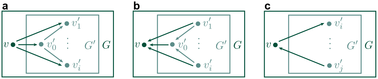
Homologies of directed subgraphs. a, b, and c illustrate three subgraphs whose homology groups or homology group dimensions are related to the original digraphs.

Proposition 2.2. Given a simple digraph $G=(V,E)$ that has a vertex $v$ with $n$ incoming arrows $v_0^{\prime }\to v,v_1^{\prime }\to v,\dots ,v_{n-1}^{\prime }\to v$. Note that $v$ does not have any outcoming arrows. Assume that for all $i\ge 1$, one has $v_i^{\prime }\to v_0^{\prime }$. Denote $G^{\prime }=\left(V^{\prime },E^{\prime }\right)$ be the subgraph of $G$ by removing the vertex $v$ with all adjacent edges (i.e. $V^{\prime }=V\setminus \left\{v\right\}$ and $E^{\prime }=E\setminus {\left\{v_i^{\prime }v\right\}}_{i=0}^{n-1}$). Then, one has $H_{*}\left(G\right)\cong H_{*}\left(G^{\prime }\right)$ (See Figure 1 b).

Proposition 2.3. Given a simple digraph $G=(V,E)$ that has a vertex $v$ with only one outcoming arrow $v\to v_i^{\prime }$ and only one incoming arrow $v_j^{\prime }\to v$, where $i\ne j$. Denote $G^{\prime }=\left(V^{\prime },E^{\prime }\right)$ be the subgraph of $G$ (See Figure 1 c) by removing the vertex $v$ and the adjacent edges $v\to v_i^{\prime }$ and $v_j^{\prime }\to v$ (i.e. $V^{\prime }=V\setminus \left\{v\right\}$ and $E^{\prime }=E\setminus \left\{v{v}_i^{\prime },v_j^{\prime }v\right\}$). Then

1. $dim{H}_p\left(G\right)=dim{H}_p\left(G^{\prime }\right)$ for $p\ne 2$ or for $p=\mathrm{0,1}$ if $v_j^{\prime }{v}_i^{\prime }$ is an edge/semi-edge in $G^{\prime }$.

2. If $v_j^{\prime }{v}_i^{\prime }$ is neither an edge or a semi-edge in $G^{\prime }$, but $v_j^{\prime }$ and $v_i^{\prime }$ are in the same connected component of $G^{\prime }$, then $dim{H}_1\left(G\right)=dim{H}_1\left(G^{\prime }+1\right)$, and $dim{H}_0\left(G\right)=dim{H}_0\left(G^{\prime }\right)$.

3. If $v_j^{\prime }$ and $v_i^{\prime }$ are not in the same connected component of $G^{\prime }$, then $\text{dim}{H}_1\left(G\right)=\text{dim}{H}_1\left(G^{\prime }\right)$ and $dim{H}_0\left(G\right)=dim{H}_0\left(G^{\prime }\right)-1$.

3. Path Laplacian and persistent path Laplacian.

One can extract topological invariants by introducing the persistent Betti numbers from the homology groups along the filtration of simplicial complex [43]. However, persistent Betti numbers do not capture homotopic geometric changes during filtration. Therefore, persistent topological Laplacians, including persistent Laplacian [37, 38] (persistent spectral graph) and persistent Hodge Laplacian [5], were introduced to reveal additional geometric information. Similarly, the constructions of path Laplacian and persistent path Laplacian are motivated by the earlier persistent spectral graphs [37, 38]. In this section, we first discuss the construction of path Laplacian. Then, we introduce filtration to the path complex to generate a series of digraphs, which gives rise to persistent path Laplacian.

3.1. Path Laplacian.

Recall that a chain complex of $\partial$-invariant paths is given by

$$\cdots {\Omega }_{n+1}\stackrel{{\partial }_{n+1}}{\to }{\Omega }_n\stackrel{{\partial }_n}{\to }{\Omega }_{n-1}\stackrel{{\partial }_{n-1}}{\to }{\Omega }_{n-2}\cdots \text{, }$$

where ${\Omega }_n={\Omega }_n\left(P\right)=\left\{v\in {𝒜}_n:\partial v\in {𝒜}_{n-1}\right\}$ and ${\partial }_n:={\left.\partial \right|}_{{\Omega }_n}$. Alternatively, assume $S_n:=S_n\left(P\right)$ to be the set of $n$-th elementary paths in $P$, then we define an inner product

$$\langle \cdot ,\cdot \rangle :S_n\times S_n\to \mathbb{R}$$

such that for any $e_{i_0\dots i_n},e_{j_0\dots j_n}\in S_n$, the following satisfies

$$\langle e_{i_0\dots i_n},e_{j_0\dots j_n}\rangle =\{\begin{array}{ll}1\hfill & \text{ if\hspace{0.17em}}{e}_{i_0\dots i_n}=e_{j_0\dots j_n},\hfill \\ 0\hfill & \text{ otherwise}.\hfill \end{array}$$ (22)

Let $M_n$ be a matrix representation of $\partial :{𝒜}_n\to {𝒜}_{n-1}$ with respect to the standard basis of ${𝒜}_n$ and ${𝒜}_{n-1}$. Define an inclusion map ${\iota }_n:{\Omega }_n\hookrightarrow {𝒜}_n$, then the matrix representation of ${\iota }_n$ with respect to the basis of ${\Omega }_n$ (i.e., the standard basis of ${𝒜}_n$ with the removal of generators that are not in ${\Omega }_n$) and the standard basis of ${𝒜}_n$ is denoted as $O_n$. Denote the boundary matrix representation of ${\partial }_n$ as $B_n$, then we have

$$O_{n-1}{B}_n={\tilde{M}}_n{O}_n.$$ (23)

If $O_{n-1}$ is a square matrix, then $O_n$ is actually an identity matrix, and we have

$$B_n=O_{n-1}^{-1}{\tilde{M}}_n{O}_n={\tilde{M}}_n{O}_n,$$ (24)

where ${\tilde{M}}_n$ is $M_n$ with the removal of rows that their basis are not elementary $(n-1)$-paths in $P$. Otherwise, $B_n$ is the least-square solution to Eq. (23).

Note that $B_n$ is the matrix representation of ${\partial }_n$ with respect to the basis of ${\Omega }_n$ and ${\Omega }_{n-1}$. Dual space ${\Omega }^n:=Hom\left({\Omega }_n,\mathbb{K}\right)$ of ${\Omega }_n$ is equipped with dual maps $d$ to form a cochain complex

$$\cdots {\Omega }^{n+1}\stackrel{d_{n+1}}{\leftarrow }{\Omega }^n\stackrel{d_n}{\leftarrow }{\Omega }^{n-1}\stackrel{d_{n-1}}{\leftarrow }{\Omega }^{n-2}\cdots ,$$

where $d_n$ is called a coboundary operator. The inner product on ${\Omega }_n$ induces an inner product $\ll \cdot ,\cdot \gg$ on ${\Omega }^n$ such that

$$\ll f,g\gg =\sum _{e\in S_n}f(e)g(e),\forall f,g\in {\Omega }^n.$$

We denote the adjoint operator of ${\partial }_n$ be ${\partial }_n^{*}:{\Omega }_{n-1}\to {\Omega }_n$. Note that similar inner product $\ll \cdot ,\cdot \gg$ on ${\Omega }^n$ was defined in the literature [23]. Hence, the coboundary operator $d_n$ is consistent with the adjoint operator ${\partial }_n^{*}$. Then, for integers $p\ge 0$, the $n$-th path Laplacian operator is a linear operator: ${\Delta }_n:{\Omega }_n\to {\Omega }_n$ given by

$${\Delta }_n={\partial }_{n+1}{\partial }_{n+1}^{*}+{\partial }_n^{*}{\partial }_n,$$ (25)

and ${\Delta }_0={\partial }_1{\partial }_1^{*}$. The $n$-th path Laplacian matrix corresponding to ${\Delta }_n$ is expressed by

$$L_n=B_{n+1}{B}_{n+1}^T+B_n^T{B}_n.$$ (26)

Since $L_n$ is positive semi-definite and symmetric, its eigenvalues are all real and non-negative. Additionally, recall that the Betti number ${\beta }_n$ of path complex $P$ satisfies

$${\beta }_n=\text{dim\hspace{0.17em}ker\hspace{0.17em}}{\partial }_n-\text{dim\hspace{0.17em}im\hspace{0.17em}}{\partial }_{n+1}=\text{dim\hspace{0.17em}ker\hspace{0.17em}}{\Delta }_n.$$ (27)

It is easy to show that

$${\beta }_n=\text{nullity}\left(L_n\right)=\text{the number of zero eigenvalues of }{L}_n.$$ (28)

Moreover, assume the dimension of $L_n$ is $𝒩$, then the set of spectra of $L_n$ is denoted as

$$\text{Spectra}\left(L_n\right)=\left\{{\left({\lambda }_1\right)}_n,{\left({\lambda }_2\right)}_n,\cdots ,{\left({\lambda }_N\right)}_n\right\}.$$

Figure 2 shows 5 digraphs with multiple vertices and directed edges. Here, we take them as examples to give a detailed illustration of $L_n$ matrix constructions.

Figure 2.

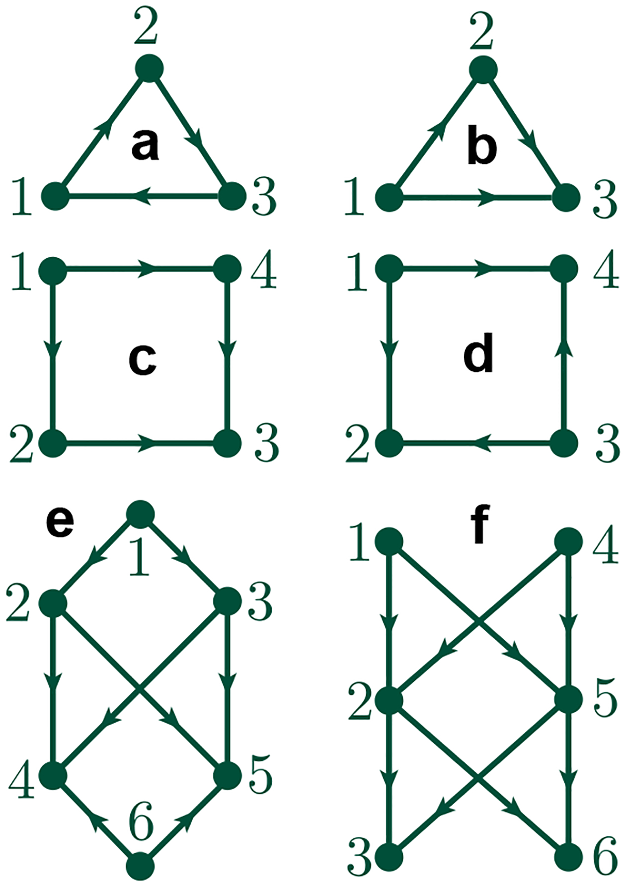
Five digraphs. a and b Digraphs with 3 vertices and 3 directed edges. c and d Digraphs with 4 vertices and 4 directed edges. e A digraph with 6 vertices and 8 directed edges. f A digraph with 6 vertices and 8 directed edges.

Construction of $L_0$ − Figure 2a Since $L_0=B_1{B}_1^T$, then we first construct $B_1$, where $B_1=O_0^{-1}{\tilde{M}}_1{O}_1$ according to Eq. (24), we have $O_0=\begin{array}{c}\\ e_1\\ e_2\\ e_3\end{array}\begin{array}{c}\begin{array}{ccc}{e}_1& e_2& e_3\end{array}\\ \left(\begin{array}{ccc}1& 0& 0\\ 0& 1& 0\\ 0& 0& 1\end{array}\right)\end{array}$, $M_1=\begin{array}{c}\\ e_1\\ e_2\\ e_3\end{array}\begin{array}{c}\begin{array}{ccc}{e}_{12}& e_{23}& e_{31}\end{array}\\ \left(\begin{array}{ccc}-1& 0& 1\\ 1& -1& 0\\ 0& 1& -1\end{array}\right)\end{array}$, and $O_1=\begin{array}{c}\\ e_{12}\\ e_{23}\\ e_{31}\end{array}\begin{array}{c}\begin{array}{ccc}{e}_{12}& e_{23}& e_{31}\end{array}\\ \left(\begin{array}{ccc}1& 0& 0\\ 0& 1& 0\\ 0& 0& 1\end{array}\right)\end{array}$. Since $e_1,e_2,e_3$ are all elementary 0-paths (vertices), $M_1={\tilde{M}}_1$. We have $B_1=O_0^{-1}{\tilde{M}}_1{O}_1=\begin{array}{c}\\ e_1\\ e_2\\ e_3\end{array}\begin{array}{c}\begin{array}{ccc}{e}_{12}& e_{23}& e_{31}\end{array}\\ \left(\begin{array}{ccc}-1& 0& 1\\ 1& -1& 0\\ 0& 1& -1\end{array}\right)\end{array}$. Then $L_0=B_1{B}_1^T=\left(\begin{array}{ccc}2& -1& -1\\ -1& 2& -1\\ -1& -1& 2\end{array}\right)$, which gives Spectra $\left(L_0\right)=\{\mathrm{0,3},3\}$ and thus, one finally has ${\beta }_0=1$.

Construction of $L_1$ − Figure 2a We have $L_1=B_2{B}_2^T+B_1^T{B}_1$, where $B_1$ has been formed, so we focus on the construction of $B_2=O_1^{-1}{\tilde{M}}_2{O}_2$ according to Eq. (24). Since $O_1=\begin{array}{c}\\ e_{12}\\ e_{23}\\ e_{31}\end{array}\begin{array}{c}\begin{array}{ccc}{e}_{12}& e_{23}& e_{31}\end{array}\\ \left(\begin{array}{ccc}1& 0& 0\\ 0& 1& 0\\ 0& 0& 1\end{array}\right)\end{array}$, $M_2=\begin{array}{c}\\ e_{11}\\ e_{12}\\ e_{13}\\ e_{21}\\ e_{22}\\ e_{23}\\ e_{31}\\ e_{32}\\ e_{33}\end{array}\begin{array}{c}\begin{array}{ccc}{e}_{123}& e_{231}& e_{312}\end{array}\\ \left(\begin{array}{ccc}0& 0& 0\\ 1& 0& 1\\ -1& 0& 0\\ 0& -1& 0\\ 0& 0& 0\\ 1& 1& 0\\ 0& 1& 1\\ 0& 0& -1\\ 0& 0& 0\end{array}\right)\end{array}$, and $O_2$ is a $3\times 0$ empty matrix since ${\Omega }_2=\left\{0\right\}$. Therefore, $B_2=O_1^{-1}{\tilde{M}}_2{O}_2$ is a $3\times 0$ empty matrix. Additionally, $L_1=B_2{B}_2^T+B_1^T{B}_1=\left(\begin{array}{ccc}2& -1& -1\\ -1& 2& -1\\ -1& -1& 2\end{array}\right)$, where $\text{Spectra}\left(L_1\right)=\{\mathrm{0,3},3\}$ and thus, one finally has ${\beta }_1=1$.

Construction of $L_2$ − Figure 2a We have $L_2=B_3{B}_3^T+B_2^T{B}_2$, where $B_2$ is an empty matrix. Hence, we focus on the construction of $B_3=O_2^{-1}{\tilde{M}}_3{O}_3$ according to Eq. (24). We have ${𝒜}_2=\text{span}\left\{e_{123},e_{231},e_{312}\right\}$ and ${𝒜}_1=\text{span}\left\{e_{12},e_{23},e_{31}\right\}$. Note that ${\partial }_2\left(e_{123}\right)=e_{23}-e_{13}+e_{12}$ where $e_{13}$ is not in ${𝒜}_1$. Hence, $e_{123}$ is not in ${\Omega }_2$. The same conclusion can be deduced for $e_{231}$ and $e_{312}$. Therefore, we have ${\Omega }_2=\left\{0\right\}$, and it is straightforward to get that $L_2$ is an empty matrix.

Construction of $L_0$ − Figure 2b Since $L_0=B_1{B}_1^T$, then we should first construct $B_1$, where $B_1=O_0^{-1}{\tilde{M}}_1{O}_1$ according to Eq. (24). Since $O_0=\begin{array}{c}\\ e_1\\ e_2\\ e_3\end{array}\begin{array}{c}\begin{array}{ccc}{e}_1& e_2& e_3\end{array}\\ \left(\begin{array}{ccc}1& 0& 0\\ 0& 1& 0\\ 0& 0& 1\end{array}\right)\end{array}$, $M_1=\begin{array}{c}\\ e_1\\ e_2\\ e_3\end{array}\begin{array}{c}\begin{array}{ccc}{e}_{12}& e_{13}& e_{23}\end{array}\\ \left(\begin{array}{ccc}-1& -1& 0\\ 1& 0& -1\\ 0& 1& 1\end{array}\right)\end{array}$, and $O_1=\begin{array}{c}\\ e_{12}\\ e_{13}\\ e_{23}\end{array}\begin{array}{c}\begin{array}{ccc}{e}_{12}& e_{13}& e_{23}\end{array}\\ \left(\begin{array}{ccc}1& 0& 0\\ 0& 1& 0\\ 0& 0& 1\end{array}\right)\end{array}$. Since $e_1,e_2$, and $e_3$ are all elementary 0-paths (vertices). Therefore, $M_1={\tilde{M}}_1$, and we have $B_1=O_0^{-1}{\tilde{M}}_1{O}_1=\begin{array}{c}\\ e_1\\ e_2\\ e_3\end{array}\begin{array}{c}\begin{array}{ccc}{e}_{12}& e_{13}& e_{23}\end{array}\\ \left(\begin{array}{ccc}-1& -1& 0\\ 1& 0& -1\\ 0& 1& 1\end{array}\right)\end{array}$. Then $L_0=B_1{B}_1^T=\left(\begin{array}{ccc}2& -1& -1\\ -1& 2& -1\\ -1& -1& 2\end{array}\right)$, which gives the $\text{Spectra}\left(L_0\right)=\{\mathrm{0,3},3\}$ and thus, one finally has ${\beta }_0=1$.

Construction of $L_1$ − Figure 2b We have $L_1=B_2{B}_2^T+B_1^T{B}_1$, where $B_1$ has been formed, so we focus on the construction of $B_2=O_1^{-1}{\tilde{M}}_2{O}_2$ according to Eq. (24). First, ${𝒜}_2=\text{span}\left\{e_{123}\right\}$ and ${𝒜}_1=\text{span}\left\{e_{12},e_{13},e_{23}\right\}$. Note that ${\partial }_2\left(e_{123}\right)=e_{23}-e_{13}+e_{12}$ where $e_{12},e_{23}$, and $e_{13}$ are all in ${𝒜}_1$. Hence, ${\Omega }_2={𝒜}_2=\text{span}\left\{e_{123}\right\}$. Note that $O_1=\begin{array}{c}\\ e_{12}\\ e_{13}\\ e_{23}\end{array}\begin{array}{c}\begin{array}{ccc}{e}_{12}& e_{13}& e_{23}\end{array}\\ \left(\begin{array}{ccc}1& 0& 0\\ 0& 1& 0\\ 0& 0& 1\end{array}\right)\end{array}$, $M_2=\begin{array}{c}\\ e_{11}\\ e_{12}\\ e_{13}\\ e_{21}\\ e_{22}\\ e_{23}\\ e_{31}\\ e_{32}\\ e_{33}\end{array}\begin{array}{c}{e}_{123}\\ \left(\begin{array}{c}0\\ 1\\ -1\\ 0\\ 0\\ 1\\ 0\\ 0\\ 0\end{array}\right)\end{array}$, and $O_2=\begin{array}{c}\\ e_{123}\end{array}\begin{array}{c}{e}_{123}\\ \left(1\right)\end{array}$. The $e_{11},e_{21},e_{22},e_{31},e_{32}$, and $e_{33}$ are not elementary 1-paths in $P$. Hence, ${\tilde{M}}_2=\begin{array}{c}\\ e_{12}\\ e_{13}\\ e_{23}\end{array}\begin{array}{c}{e}_{123}\\ \left(\begin{array}{c}1\\ -1\\ 1\end{array}\right)\end{array}$, and then $B_2=O_1^{-1}{\tilde{M}}_2{O}_2=\begin{array}{c}\\ e_{12}\\ e_{13}\\ e_{23}\end{array}\begin{array}{c}{e}_{123}\\ \left(\begin{array}{c}1\\ -1\\ 1\end{array}\right)\end{array}$. Therefore, $L_1=B_2{B}_2^T+B_1^T{B}_1=\left(\begin{array}{ccc}3& 0& 0\\ 0& 3& 0\\ 0& 0& 3\end{array}\right)$, where $\text{Spectra}\left(L_1\right)=\{\mathrm{3,3},3\}$ and thus, we finally have ${\beta }_1=0$.

Construction of $L_2$ − Figure 2b According to Eq. (26), we have $L_2=B_3{B}_3^T+B_2^T{B}_2$ and $B_3=O_2^{-1}{\tilde{M}}_3{O}_3$. Since there is no 3-path existing, so the $M_3$ and $O_3$ are both empty matrix. Hence $L_2=\left(3\right),\text{Spectra}\left(L_2\right)=\left\{3\right\}$, and thus, one has ${\beta }_2=0$.

In the following section, we will omit the detailed construction steps of boundary matrix $B_n$. Table 1, Table 2, Table 3, and Table 4 list the boundary matrix $B_n$ and the $n$-th path Laplacian matrix $L_n$ for with its corresponding Betti numbers ${\beta }_n$ and spectrum $\text{Spectra}\left(L_n\right)$ for Figure 2 c, d, e, and f. It is worth to mention that ${\beta }_n$ can distinguish the same graph with different paths assigned. For example, Figure 2 c and d have the same undirected graph structure with different paths assigned. We have ${\beta }_1=0$ for Figure 2 c and ${\beta }_1=1$ for Figure 2 d.

Table 1.

Illustration of digraph c in Figure 2

$n$	$n=0$	$n=1$	$n=2$
${\Omega }_n$	$\text{span}\left\{e_1,e_2,e_3,e_4\right\}$	$\text{span}\left\{e_{12},e_{14},e_{23},e_{43}\right\}$	$\text{span}\left\{e_{143}-e_{123}\right\}$
$B_{n+1}$	$\begin{array}{c}\\ e_1\\ e_2\\ e_3\\ e_4\end{array}\begin{array}{c}\begin{array}{cccc}{e}_{12}& e_{14}& e_{23}& e_{43}\end{array}\\ \left(\begin{array}{cccc}-1& -1& 0& 0\\ 1& 0& -1& 0\\ 0& 0& 1& 1\\ 0& 1& 0& -1\end{array}\right)\end{array}$	$\begin{array}{c}\\ e_{12}\\ e_{14}\\ e_{23}\\ e_{43}\end{array}\begin{array}{c}{e}_{143}-e_{123}\\ \left(\begin{array}{c}-1\\ 1\\ -1\\ 1\end{array}\right)\end{array}$	$1\times 0$ empty matrix
$L_n$	$\left(\begin{array}{cccc}2& -1& 0& -1\\ -1& 2& -1& 0\\ 0& -1& 2& -1\\ -1& 0& -1& 2\end{array}\right)$	$\left(\begin{array}{cccc}3& 0& 0& -1\\ 0& 3& -1& 0\\ 0& -1& 3& 0\\ -1& 0& 0& 3\end{array}\right)$	(4)
${\beta }_n$	1	0	0
$\text{Spectra}\left(L_n\right)$	{0, 2, 2, 4}	{2, 2, 4, 4}	{4}

Table 2.

Illustration of digraph d in Figure 2

$n$	$n=0$	$n=1$	$n=2$
Ωn	$\text{span}\left\{e_1,e_2,e_3,e_4\right\}$	$\text{span}\left\{e_{12},e_{14},e_{32},e_{34}\right\}$	{0}
$B_{n+1}$	$\begin{array}{c}\\ e_1\\ e_2\\ e_3\\ e_4\end{array}\begin{array}{c}\begin{array}{cccc}{e}_{12}& e_{14}& e_{32}& e_{34}\end{array}\\ \left(\begin{array}{cccc}-1& -1& 0& 0\\ 1& 0& 1& 0\\ 0& 0& -1& -1\\ 0& 1& 0& 1\end{array}\right)\end{array}$	$4\times 0$ empty matrix	(/)
$L_n$	$\left(\begin{array}{cccc}2& -1& 0& -1\\ -1& 2& -1& 0\\ 0& -1& 2& -1\\ -1& 0& -1& 2\end{array}\right)$	$\left(\begin{array}{cccc}2& 1& 1& 0\\ 1& 2& 0& 1\\ 1& 0& 2& 1\\ 0& 1& 1& 2\end{array}\right)$	(/)
${\beta }_n$	1	1	0
$\text{Spectra}\left(L_n\right)$	{0, 2, 2, 4}	{0, 2, 4, 4}	/

Table 3.

Illustration of digraph e in Figure 2.

$n$	$n=0$	$n=1$	$n=2$
${\Omega }_n$	$\text{span}\left\{e_1,e_2,e_3,e_4,e_5,e_6\right\}$	$\text{span}\left\{e_{12},e_{13},e_{24},e_{25},e_{34},e_{35},e_{64},e_{65}\right\}$	$\text{span}\left\{e_{134}-e_{124},e_{135}-e_{125}\right\}$
$B_{n+1}$	$\begin{array}{c}\\ e_1\\ e_2\\ e_3\\ e_4\\ e_5\\ e_6\end{array}\begin{array}{c}\begin{array}{cccccccc}{e}_{12}& e_{13}& e_{24}& e_{25}& e_{34}& e_{35}& e_{64}& e_{65}\end{array}\\ \left(\begin{array}{cccccccc}-1& -1& 0& 0& 0& 0& 0& 0\\ 1& 0& -1& -1& 0& 0& 0& 0\\ 0& 1& 0& 0& -1& -1& 0& 0\\ 0& 0& 1& 0& 1& 0& 1& 0\\ 0& 0& 0& 1& 0& 1& 0& 1\\ 0& 0& 0& 0& 0& 0& -1& -1\end{array}\right)\end{array}$	$\begin{array}{c}\\ e_{12}\\ e_{13}\\ e_{24}\\ e_{25}\\ e_{34}\\ e_{35}\\ e_{64}\\ e_{65}\end{array}\begin{array}{c}\begin{array}{cc}{e}_{134}-e_{124}& e_{135}-e_{125}\end{array}\\ \left(\begin{array}{cc}-1& -1\\ 1& 1\\ -1& 0\\ 0& -1\\ 1& 0\\ 0& 1\\ 0& 0\\ 0& 0\end{array}\right)\end{array}$	$2\times 0$ empty matrix
$L_n$	$\left(\begin{array}{cccccc}2& -1& -1& 0& 0& 0\\ -1& 3& 0& -1& -1& 0\\ -1& 0& 3& -1& -1& 0\\ 0& -1& -1& 3& 0& -1\\ 0& -1& -1& 0& 3& -1\\ 0& 0& 0& -1& -1& 2\end{array}\right)$	$\left(\begin{array}{cccccccc}4& -1& 0& 0& -1& -1& 0& 0\\ -1& 4& -1& -1& 0& 0& 0& 0\\ 0& -1& 3& 1& 0& 0& 1& 0\\ 0& -1& 1& 3& 0& 0& 0& 1\\ -1& 0& 0& 0& 3& 1& 1& 0\\ -1& 0& 0& 0& 1& 3& 0& 1\\ 0& 0& 1& 0& 1& 0& 2& 1\\ 0& 0& 0& 1& 0& 1& 1& 2\end{array}\right)$	$\left(\begin{array}{cc}4& 2\\ 2& 4\end{array}\right)$
${\beta }_n$	1	1	0
$\text{Spectra}\left(L_n\right)$	{0, 1.4384, 3, 3, 3, 5}	{0, 1.4384, 2, 3, 3, 3, 5.5616, 6}	{2,6}

Table 4.

Illustration of digraph f in Figure 2.

$n$	$n=0$	$n=1$	$n=2$
${\Omega }_n$	$\text{span}\left\{e_1,e_2,e_3,e_4,e_5,e_6\right\}$	$\text{span}\left\{e_{12},e_{15},e_{23},e_{26},e_{42},e_{45},e_{53},e_{56}\right\}$	$\text{span}\{e_{153}-e_{123},e_{156}-e_{126},e_{453}-e_{423},e_{456}-e_{426}\}$
$B_{n+1}$	$\begin{array}{c}\\ e_1\\ e_2\\ e_3\\ e_4\\ e_5\\ e_6\end{array}\begin{array}{c}\begin{array}{cccccccc}{e}_{12}& e_{15}& e_{23}& e_{26}& e_{42}& e_{45}& e_{53}& e_{56}\end{array}\\ \left(\begin{array}{cccccccc}-1& -1& 0& 0& 0& 0& 0& 0\\ 1& 0& -1& -1& 1& 0& 0& 0\\ 0& 0& 1& 0& 0& 0& 1& 0\\ 0& 0& 0& 0& -1& -1& 0& 0\\ 0& 1& 0& 0& 0& 1& -1& -1\\ 0& 0& 0& 1& 0& 0& 0& 1\end{array}\right)\end{array}$	$\begin{array}{c}\\ e_{12}\\ e_{15}\\ e_{23}\\ e_{26}\\ e_{42}\\ e_{45}\\ e_{53}\\ e_{56}\end{array}\begin{array}{c}\begin{array}{cccc}{e}_{153}-e_{123}& e_{156}-e_{126}& e_{453}-e_{423}& e_{456}-e_{426}\end{array}\\ \left(\begin{array}{cccc}-1& -1& 0& 0\\ 1& 1& 0& 0\\ -1& 0& -1& 0\\ 0& -1& 0& -1\\ 0& 0& -1& -1\\ 0& 0& 1& 1\\ 1& 0& 1& 0\\ 0& 1& 0& 1\end{array}\right)\end{array}$	$4\times 0$ empty matrix
$L_n$	$\left(\begin{array}{cccccc}2& -1& 0& 0& -1& 0\\ -1& 4& -1& -1& 0& -1\\ 0& -1& 2& 0& -1& 0\\ 0& -1& 0& 2& -1& 0\\ -1& 0& -1& -1& 4& -1\\ 0& -1& 0& 0& -1& 2\end{array}\right)$	$\left(\begin{array}{cccccccc}4& -1& 0& 0& 1& 0& -1& -1\\ -1& 4& -1& -1& 0& 1& 0& 0\\ 0& -1& 4& 1& 0& -1& -1& 0\\ 0& -1& 1& 4& 0& -1& 0& -1\\ 1& 0& 0& 0& 4& -1& -1& -1\\ 0& 1& -1& -1& -1& 4& 0& 0\\ -1& 0& -1& 0& -1& 0& 4& 1\\ -1& 0& 0& -1& -1& 0& 1& 4\end{array}\right)$	$\left(\begin{array}{cccc}4& 2& 2& 0\\ 2& 4& 0& 2\\ 2& 0& 4& 2\\ 0& 2& 2& 4\end{array}\right)$
${\beta }_n$	1	0	1
$\text{Spectra}\left(L_n\right)$	{0, 2, 2, 2, 4, 6}	{2, 2, 2, 4, 4, 4, 6, 8}	{0, 4, 4, 8}

3.2. Persistent path Laplacian.

From Section 3.1, the way to calculate both harmonic spectra (topological invariants) and non-harmonic spectra of $n$-th path Laplacian matrix is genuinely free of metrics or coordinates, which contains too little information to fully describe the object. Therefore, inspired by the idea of the persistent spectral graph (PSG), persistent path Laplacian (PPL) is proposed to create a sequence of digraphs induced by varying a filtration parameter to encode more geometric or structural information.

First, we consider a filtration of digraphs $𝒢:\mathbb{R}\to 𝒟$, which is a morphism $f_{s,t}:H_p\left({𝒢}_t;\mathbb{K}\right)\to H_p\left({𝒢}_s;\mathbb{K}\right)$ from the category of real number $\mathbb{R}$ to the category of digraphs $𝒟$ that satisfies:

$$𝒢(t)\subseteq 𝒢(s),\forall t\le s,$$

where $G_t:=𝒢\left(t\right)\in 𝒟$ and $G_s:=𝒢\left(s\right)\in 𝒟$. Consider a sequence of finitely many positive integers $\mathrm{1,2},\dots ,m$, we have a sequence of digraphs

$$G_1\subseteq G_2\subseteq \cdots \subseteq G_m.$$

For each digraph $G_t$, we denote its corresponding chain group to be ${\Omega }_n\left(G_t\right)$, and the $n$-boundary operator of $G_t$ is denoted by ${\partial }_n^t:{\Omega }_n\left(G_t\right)\to {\Omega }_{n-1}\left(G_t\right),\forall n\ge 0$.

Similarly, as in persistent homology, a sequence of chain complexes can be denoted as

$$\begin{array}{cccccccccccccc}\cdots & {\Omega }_{n+1}^1& \stackrel{{\partial }_{n+1}^1}{\to }& {\Omega }_n^1& \stackrel{{\partial }_n^1}{\to }& \cdots & \stackrel{{\partial }_3^1}{\to }& {\Omega }_2^1& \stackrel{{\partial }_2^1}{\to }& {\Omega }_1^1& \stackrel{{\partial }_1^1}{\to }& {\Omega }_0^1& \stackrel{{\partial }_0^1}{\to }& {\Omega }_{-1}^1\\ & \downarrow & & \downarrow & & & & \downarrow & & \downarrow & & \downarrow & & \\ \cdots & {\Omega }_{n+1}^2& \stackrel{{\partial }_{q+1}^2}{\to }& {\Omega }_n^2& \stackrel{{\partial }_n^2}{\to }& \cdots & \stackrel{{\partial }_3^2}{\to }& {\Omega }_2^2& \stackrel{{\partial }_2^2}{\to }& {\Omega }_1^2& \stackrel{{\partial }_1^2}{\to }& {\Omega }_0^2& \stackrel{{\partial }_0^2}{\to }& {\Omega }_{-1}^2\\ & ⋮& & ⋮& & & & ⋮& & ⋮& & ⋮& & \\ & \downarrow & & \downarrow & & & & \downarrow & & \downarrow & & \downarrow & & \\ \cdots & {\Omega }_{n+1}^m& \stackrel{{\partial }_{q+1}^m}{\to }& {\Omega }_n^m& \stackrel{{\partial }_n^m}{\to }& \cdots & \stackrel{{\partial }_3^n}{\to }& {\Omega }_2^m& \stackrel{{\partial }_2^m}{\to }& {\Omega }_1^m& \stackrel{{\partial }_1^m}{\to }& {\Omega }_0^m& \stackrel{{\partial }_0^m}{\to }& {\Omega }_{-1}^m\end{array}$$ (29)

For the sake of simplicity, we use ${\Omega }_n^t$ to represent ${\Omega }_n\left(G_t\right)$. Suppose a subset of ${\Omega }_n^s$ whose boundary is in ${\Omega }_{n-1}^t$ as:

$${\Omega }_n^{t,s}:=\left\{\alpha \in {\Omega }_n^s\mid {\partial }_n^s\alpha \in {\Omega }_{n-1}^t\right\}.$$ (30)

The persistent $n$-boundary operator is denoted as ${ð}_n^{t,s}:{\Omega }_n^{t,s}\to {\Omega }_{n-1}^t$, and its corresponding adjoint operator is ${\left({ð}_n^{t,s}\right)}^{*}:{\Omega }_{n-1}^t\to {\Omega }_n^{t,s}$. Therefore, the persistent $n$-th path Laplacian operator ${\Delta }_n^{t,s}:{\Omega }_n^t\to {\Omega }_n^t$ defined along the filtration is:

$${\Delta }_n^{t,s}={ð}_{n+1}^{t,s}{\left({ð}_{n+1}^{t,s}\right)}^{*}+{\partial }_n^{t^{*}}{\partial }_n^t.$$ (31)

Since ${\Delta }_n^{t,s}$ inherits the inner product from ${ð}_{n+1}^{t,s}$, then the adjoint map $\left({ð}_{n+1}^{t,s}\right)$ well defined. Intuitively, the matrix representation of ${\Delta }_n^{t,s}$ is

$$L_n^{t,s}=B_{n+1}^{t,s}{P}^{-1}{\left(B_{n+1}^{t,s}\right)}^T+{\left(B_n^t\right)}^T{B}_n^t,$$ (32)

where $P^{-1}$ is the associated inner product matrix of ${\Omega }_{n+1}^{t,s}$ with arbitrary basis. Moreover, assume the dimension of $L_n^{t,s}$ is $N$, then the spectra of $L_n^{t,s}$ that are arranged in ascending order can be displayed as:

$$\text{Spectra}\left(L_n^{t,s}\right)=\left\{{\left({\lambda }_1\right)}_n^{t,s},{\left({\lambda }_2\right)}_n^{t,s},\cdots ,{\left({\lambda }_N\right)}_n^{t,s}\right\}.$$

Note that the smallest non-harmonic spectra of $L_n^{t,s}$ is denoted as ${\left({\tilde{\lambda }}_2\right)}_n^{t,s}$. We call the multiplicity of zero spectra of $L_q^{t,s}$ to be persistent $n$-th Betti number ${\beta }_n^{t,s}$ from $G_t$ to $G_s$.

$$\begin{gathered} {\beta }_n^{t,s}=\text{nullity}\left(L_n^{t,s}\right) \\ =\text{the number of zero eigenvalues }(\text{i}.\text{e}.,\text{ harmonic eigenvalues})\text{ of }{L}_n^{t,s}. \end{gathered}$$ (33)

Distanced-based filtration

Specifically, suppose $G\left(w\right)=(V,E,w)$ is a weighted digraph, where $V$ is the set of the vertices and $E$ is the set of the directed edges. Assume $w$ is a weight function $w:E\to \mathbb{R}$. For example, if $V$ is in the Euclidean space, then a digraph $G\left(w\right)$ is a geometric digraph (a geometric digraph is a digraph in which the vertices are embedded as points in the Euclidean space, and the edges are embedded as non-crossing directed line segments). For any $(i,j)\in E$ where $i,j\in V$, we define $w\left(i,j\right)=\parallel i-j\parallel$, where $\parallel \cdot \parallel$ is a Euclidean metric. Hence, for every $\delta \in \mathbb{R}$, a digraph can be described as $G^{\delta }=\left(V,E^{\delta }\right)=(V,\{e\in E:w\left(e\right)\le \delta \left\}\right)$, and a filtration of digraphs can be described as ${\left\{G^{\delta }\hookrightarrow G^{{\delta }^{\prime }}\right\}}_{\delta \le {\delta }^{\prime }}$.

Therefore, the persistent $n$-th path Laplacian matrix defined on the filtration is

$$L_n^{\delta ,{\delta }^{\prime }}=B_{n+1}^{\delta ,{\delta }^{\prime }}{P}^{-1}{\left(B_{n+1}^{\delta ,{\delta }^{\prime }}\right)}^T+{\left(B_n^{\delta }\right)}^T{B}_n^{\delta },$$ (34)

where its corresponding Betti numbers and spectra can be expressed as:

$$\begin{gathered} {\beta }_n^{\delta ,{\delta }^{\prime }}=\text{nullity}\left(L_n^{\delta ,{\delta }^{\prime }}\right) \\ =\text{the number of zero eigenvalues }(\text{i}.\text{e}.,\text{ harmonic eigenvalues})\text{ of }{L}_n^{\delta ,{\delta }^{\prime }}. \end{gathered}$$ (35)

$$\text{Spectra}\left(L_n^{\delta ,{\delta }^{\prime }}\right)=\left\{{\left({\lambda }_1\right)}_n^{\delta ,{\delta }^{\prime }},{\left({\lambda }_2\right)}_n^{\delta ,{\delta }^{\prime }},\cdots ,{\left({\lambda }_N\right)}_n^{\delta ,{\delta }^{\prime }}\right\}.$$ (36)

Notably, the Fiedler value (i.e., spectral gap) of $L_n^{\delta ,{\delta }^{\prime }}$ is widely used in many other areas such as physics and geography, which is denoted as ${\tilde{\lambda }}_n^{\delta ,{\delta }^{\prime }}$. As shown below, it is sensitive to both topological and geometric changes.

Moreover, it is worth to mention that isolated points (vertices) can be either included in the digraphs (under the distance-based filtration) or removed from the digraphs (under the distanced-based filtration with removal of isolated points).

One can get both abstract information (revealed by Betti numbers) and geometric information (revealed by non-harmonic spectra) from digraphs along filtration. For instance, Figure 3 illustrates the filtration on two tetrahedrons. The top panel is a tetrahedron (Tetra 1) with edge lengths $\left|e_{12}\right|=\left|e_{32}\right|=\left|e_{24}\right|=1$, and $\left|e_{13}\right|=\left|e_{14}\right|=\left|e_{34}\right|=\sqrt{2}$. The bottom panel is another tetrahedron (Tetra 2) with edge lengths $\left|e_{12}\right|=\sqrt{3},\left|e_{32}\right|=\left|e_{24}\right|=1$, and $\left|e_{13}\right|=\left|e_{14}\right|=2$, and $\left|e_{34}\right|=\sqrt{2}$. We say $G_1=G^0,G_2=G^1,G_3=G^{\sqrt{2}},G_4=G^{\sqrt{3}}$, and $G_5=G^{\sqrt{5}}$. Figure 4 shows the changes of ${\beta }_n^{\delta ,\delta }$ and ${\lambda }_n^{\delta ,\delta }$ of persistent $n$-th path Laplacian $L_n^{\delta ,\delta }$ along filtration. It can be seen that by varying the filtration parameter $\delta$ from 0 to 1, the Betti 1 and Betti 2 are always 0. However, the smallest nonzero eigenvalue ${\tilde{\lambda }}_n^{\delta ,\delta }$ of Tetra 1 and Tetra 2 have changes along filtration parameter $\delta$. Additionally, when $n=\mathrm{1,2}$, the ${\tilde{\lambda }}_n^{\delta ,\delta }$ can distinguish Tetra 1 and Tetra 2, while ${\beta }_n^{\delta ,\delta }$ cannot. This indicates that non-harmonic spectra of persistent path Laplacian can reveal more geometric information than the persistent Betti numbers in distinguishing similar topological structures. Notably, we remove all the isolated points from each digraph for the simplicity of calculation.

Figure 3.

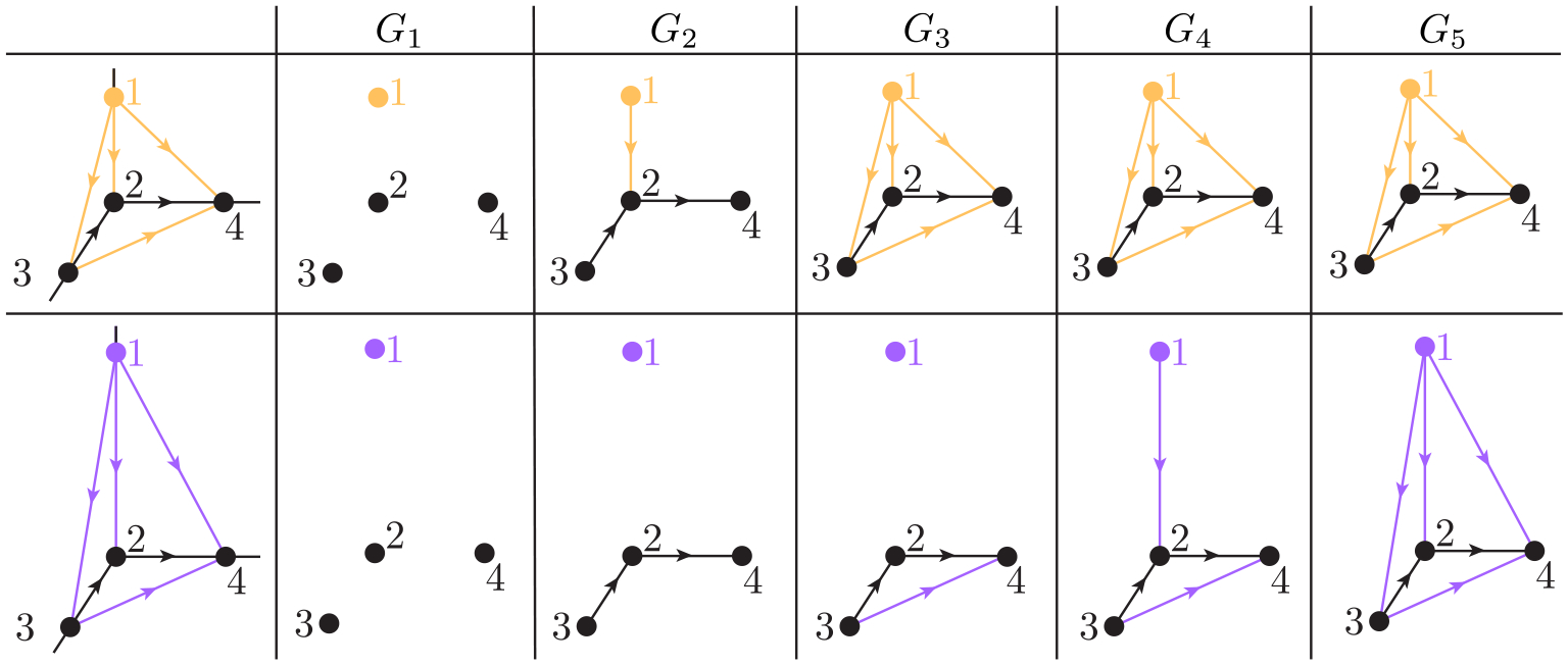
Illustration of filtration on a tetrahedron. Here, 1,2,3, and 4 represent four elementary 0-paths $e_1,e_2,e_3$, and $e_4$. The top panel is a tetrahedron that has edge lengths $\left|e_{12}\right|=\left|e_{32}\right|=\left|e_{24}\right|=1$ and $\left|e_{13}\right|=\left|e_{14}\right|=\left|e_{34}\right|=\sqrt{2}$. The bottom panel is a tetrahedron that has edge lengths $\left|e_{32}\right|=\left|e_{24}\right|=1$, $\left|e_{34}\right|=\sqrt{2}$, $\left|e_{12}\right|=\sqrt{3}$, and $\left|e_{13}\right|=\left|e_{14}\right|=2$.

Figure 4.

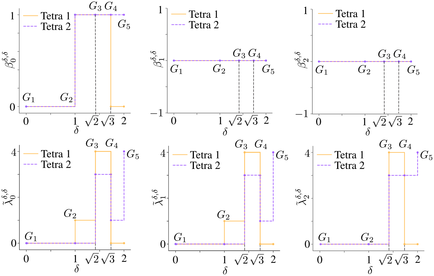
Comparison of Betti numbers and non-harmonic spectra of $L_n^{\delta ,\delta }$ when $n=\mathrm{0,1},\text{\hspace{0.17em}and\hspace{0.17em}}2$ on tetrahedrons Tetra 1 and Tetra 2. Note that since ${\beta }_1^{\delta ,\delta }=0$ and ${\beta }_2^{\delta ,\delta }=0$ for Tetra 1 and Tetra 2, topological variants from persistent path homology cannot discriminate Tetra 1 and Tetra 2. However ${\lambda }_1^{\delta ,\delta }$ and ${\lambda }_2^{\delta ,\delta }$ show the differences between Tetra 1 and Tetra 2.

Moreover, a more complicated example is also illustrated in Figure 5 to describe the filtration on two pyramids. The top panel is a pyramid (Pyra 1) with edge lengths $\left|e_{12}\right|=\left|e_{32}\right|=\left|e_{24}\right|=1$, and $\left|e_{13}\right|=\left|e_{14}\right|=\left|e_{34}\right|=\sqrt{2}$. The bottom panel is a pyramid (Pyra 2) with edge lengths $\left|e_{12}\right|=\sqrt{3},\left|e_{32},\right|=\left|e_{24}\right|=1$, and $\left|e_{13}\right|=\left|e_{14}\right|=2$, and $\left|e_{34}\right|=\sqrt{2}$. We say $G_1=G^0,G_2=G^1,G_3=G^{\sqrt{2}},G_4=G^{\sqrt{3}}$, and $G_5=G^{\sqrt{5}}$. Figure 6 depicts the changes of ${\beta }_n^{\delta ,\delta }$ and ${\lambda }_n^{\delta ,\delta }$ of persistent $n$-th path Laplacian $L_n^{\delta ,\delta }$ for objects Pyra 1 and Pyra 2 along filtration. For Pyra 1 and Pyra 2, when $n=0$ and $\delta =1$, their corresponding digraphs form, which result in ${\beta }_0^{\mathrm{1,1}}=1$ and ${\beta }_1^{\mathrm{1,1}}=1$ for both Pyra 1 and Pyra 2. When $\delta =\sqrt{3}$, we have ${\beta }_1^{\sqrt{3},\sqrt{3}}=0$ for Pyra 1 since the introducing of a new directed edges $e_{15}$. When $\delta =\sqrt{5}$, we have ${\beta }_1^{\sqrt{5},\sqrt{5}}=0$ for Pyra 2 since the introducing of a new directed edges $e_{15}$ kills the 1-cycle formed by $e_{25},e_{32},e_{34}$, and $e_{54}$. Furthermore, although Pyra 1 and Pyra 2 do not have exactly the same geometric structure, their share the same ${\beta }_2^{\delta ,\delta }$ value from $\delta =0$ to $\delta =\sqrt{5}$. However, Pyra 1 and Pyra 2 can be distinguished by the ${\tilde{\lambda }}_2^{\delta ,\delta }$ along filtration. Therefore, we can see that similar to the PSG, one can use the non-harmonic spectra from the persistent path laplacian to reveal the intrinsic geometric information of a givens point-cloud dataset by varying the filtration parameters. In addition, the detailed calculations of $L_n^{\delta ,\delta }$ can be found in the Appendix.

Figure 5.

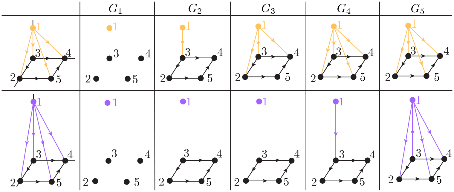
Illustration of filtration on a pyramid. Here, 1, 2, 3, 4, and 5 represent five elementary 0-paths $e_1,e_2,e_3,e_4$, and $e_5$. The top panel is a pyramid that has edge lengths $\left|e_{13}\right|=\left|e_{25}\right|=\left|e_{32}\right|=\left|e_{34}\right|=\left|e_{54}\right|=1$, $\left|e_{12}\right|=\left|e_{14}\right|=\sqrt{2}$, and $\left|e_{15}\right|=\sqrt{3}$. The bottom panel is a pyramid that has edge lengths $\left|e_{25}\right|=\left|e_{32}\right|=\left|e_{34}\right|=\left|e_{54}\right|=1$, $\left|e_{12}\right|=\left|e_{14}\right|=2$, and $\left|e_{15}\right|=\sqrt{5}$.

Figure 6.

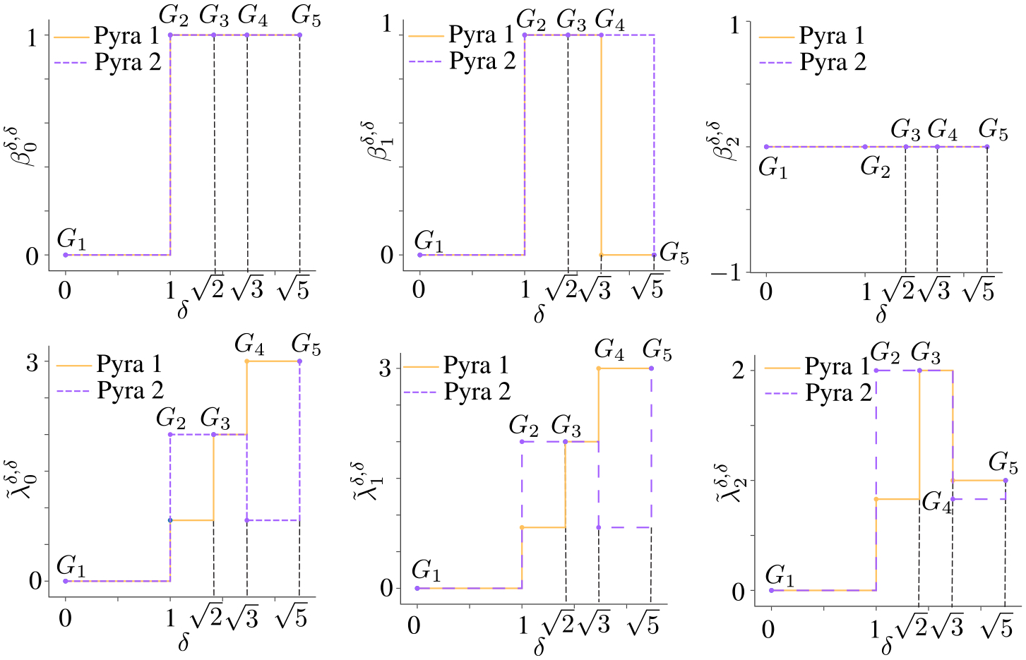
Comparison of Betti number and non-harmonic spectra of $L_n^{\delta ,\delta }$ when $n=\mathrm{0,1},c$ and 2 on pyramids Pyra 1 and Pyra 2. Note that since ${\beta }_2^{\delta ,\delta }=0$, it cannot distinguish Pyra 1 and Pyra 2. But ${\lambda }_2^{\delta ,\delta }$ can tell the difference.

4. Application.

In this section, we apply the persistent path Laplacian to the analysis of the curcurbit[n]urils system. Cucurbiturils are macrocyclic molecules, which are made of glycoluril (=C₆H₂N₄O₂=) monomers linked by methylene bridges (−CH₂−). $CBn$ is commonly used as an abbreviation of Cucurbiturils. Here, $n$ is the number of glycoluril units. In this work, we consider CB7 as an example. The molecular formulas of CB7 is C₄₂H₁₄N₂₈O₁₄. The molecular structure of CB7 is obtained from the Supporting Information of Ref. [11].

Figure 7 illustrates how PPL is employed for a molecular system to extract its rich topological and geometric information. The first two charts of Figure 7a describe the three-dimensional (3D) top view and side view of CB7. The green, blue, red, and gray colors represent C,N,O, and H atoms, respectively. The third chart of Figure 7a is a basic “Octagon-pentagon” unit that consists of two glycolurils. It can be seen that 7 glycolurils exist in CB7. The last chart of Figure 7a demonstrates the path direction assignment to pairs of atoms based on atomic electronegativity. The periodic table of electronegativity is given by the Pauling scale [30], in which the electronegativities of C,N,O, and H are 2.55, 3.04, 3.44, and 2.20, respectively. Then, we set the directions of edges following the order “H → C → N → O”.

Figure 7.

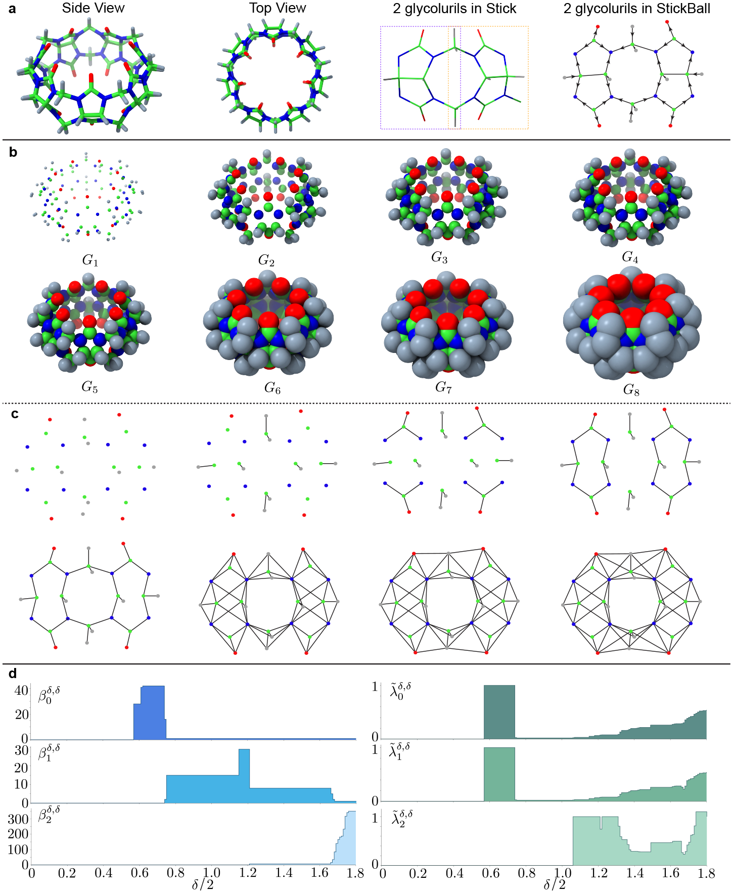
a The 3D structures of CB7, 2 glycolurils, and path direction assignment. Here, from left to right, the side view of CB7, top view of CB7, the structure of two glycoluril units (=C₁₀H₄N₈O₄=), and electronegativity-based path direction assignment are depicted as well. b Illustration of filtration-induced geometries $G_i(i=\mathrm{1,2},\dots ,8)$ of CB7. Eight digraphs $G_1=G_0^{0.200*2},G_2=G_0^{0.565*2},G_3=G_0^{0.710*2},G_4=G_0^{0.745*2},G_5=G_0^{0.800*2},G_6=G_0^{1.210*2},G_7=G_0^{1.315*2},G_8=G_0^{1.800*2}$ are constructed under filtration parameter $\delta$. c Illustration of filtration-induced path complexes within two glycoluril units. Path directions can be inferred from their colors as shown in the last chart of a d Betti numbers ${\beta }_n^{\delta ,\delta }$ and non-harmonic spectra ${\tilde{\lambda }}_n^{\delta ,\delta }$ of persistent path Laplacians $\left(L_n^{\delta ,\delta }\right.$ when $n=\mathrm{0,1}$, and 2) for CB7.

Figure 7b depicts the distance-based filtration of CB7. Here, structures $G_i(i=\mathrm{1,2},\dots ,8)$ were obtained at the filtration radii of 0.200, 0.565, 0.710, 0.745, 0.800, 1.210, 1.315, and 1.800Å, respectively. In our digraph notation, we denote these structures as $G_1=G_0^{0.200*2},G_2=G_0^{0.565*2},G_3=G_0^{0.710*2},G_4=G_0^{0.745*2},G_5=G_0^{0.800*2},G_6=G_0^{1.210*2},G_7=G_0^{1.315*2}$, and $G_8=G_0^{1.800*2}$. Note that, in the present formulation, all of the isolated points were removed from these digraphs.

Figure 7c illustrates the filtration-induced path complexes in the aforementioned $G_i(i=\mathrm{1,2},\dots ,8)$. To clearly show the topological and geometric changes, only the path complexes in one “Octagon-pentagon” unit (or two glycolurils) are considered and depicted for each structure. For simplicity, only edges are presented. However, their path directions can be easily assigned based on their color map as shown in the last chart of Figure 7a.

Figure 7d depicts the PPL spectra of CB7. We can see that at the initial state $\left(G_1\right)$ when $r=\delta /2=0.200\AA$), total 98 atoms are isolated from one another. When radius $\delta =0.565\AA \left(G_2\right)$, C atoms on each pentagon are connected with their H atom neighborhoods. Therefore, four isolated components are formed in each glycoluril, which makes ${\beta }_0^{\delta ,\delta }=4\times 7=28$. At $G_3(r=0.710\AA )$, C atoms on each pentagon are connected with their N and O neighborhoods. At this stage, two more connected components are involved in one glycoluri structure, which makes ${\beta }_0^{\delta ,\delta }=6\times 7=42$. Only one connected structure can be formed if all of the atoms get connected with their neighborhood atoms. Therefore, ${\beta }_0^{\delta ,\delta }=1$ (see $G_5-G_8$). Notably, the ${\beta }_2^{\delta ,\delta }$ and ${\tilde{\lambda }}_2^{\delta ,\delta }$ provide rich topological and geometric information when the filtration parameter $\delta$ increases.

This example shows that PPL can decode topological persistence and the shape evolution of a given molecular system with chemical- or biological-based directional assignment. Specifically, ${\tilde{\lambda }}_0^{\delta ,\delta }$ can still offer geometric information when ${\beta }_0^{\delta ,\delta }$ does not changes for large radii. Therefore, PPL keeps revealing homotopic shape evolution when the topological invariant from persistent path homology does not change.

Additionally, unlike persistent Laplacian, high-order PPL operators provide rich topological information. For instance, when the filtration parameter $r=\delta /2$ increases to $1.68,{\beta }_2^{\delta ,\delta }$ from PPL dramatically goes up. Whereas, in persistent Laplacian, the value of Betti 2 is quite limited since the CB7 system can barely form 2-cycles at a similar filtration parameter using either Rips complex or alpha complex. This trait endows PPL with a better ability to characterize the geometry and topology of an object at large scales.

5. Conclusion.

Path homology, a rich mathematical concept introduced by Grigor’yan, Lin, Muranov, and Yau, has stimulated a variety of new developments in pure and applied mathematics, including much attention from the topological data analysis (TDA) community. Unlike original homology or persistent homology, path homology enables the treatment of directed graphs and networks. Persistent path homology bridges path homology with multiscale analysis, making it a powerful tool for practical applications. Nonetheless, these formulations are insensitive to homotopic shape evolution during filtration.

Topological Laplacians, including Hodge Laplacian, graph Laplacian, sheaf Laplacian, and Dirac Laplacian, are versatile mathematical tools that not only preserve all topological invariants but also describe geometric shapes. This work introduces a new topological Laplacian, namely persistent path Laplacian, as a new mathematical tool for the multi-scale analysis of directed graphs and networks. For a given data, the proposed persistent path Laplacian fully recovers the topological persistence of persistent homology in its harmonic spectra and meanwhile, captures homotopic shape evolution of the data during filtration in its non-harmonic spectra.

Appendix.

In Tables 5–19, we present the detailed matrix constructions, Betti numbers, and spectra for various digraphs shown in Figure 5 top and bottom panels.

Table 5.

Matrix construction of graph $G_1$ (with isolated points included) in the top panel of Figure 5.

$n$	$n=0$	$n=1$	$n=2$
${\Omega }_n$	$\text{span}\left\{e_1,e_2,e_3,e_4,e_5\right\}$	{0}	{0}
$B_{n+1}$	$5\times 0$ empty matrix	/	/
$L_n$	$5\times 5$ zero matrix	/	/
${\beta }_n$	5	/	/
$\text{Spectra}\left(L_n\right)$	{0, 0, 0, 0, 0}	/	/

Table 6.

Matrix construction of graph $G_1$ (without isolated points) in the top panel of Figure 5.

$n$	$n=0$	$n=1$	$n=2$
${\Omega }_n$	{0}	{0}	{0}
$B_{n+1}$	/	/	/
$L_n$	/	/	/
${\beta }_n$	/	/	/
$\text{Spectra}\left(L_n\right)$	/	/	/

Table 7.

Matrix construction of graph $G_2$ in the top panel of Figure 5.

$n$	$n=0$	$n=1$	$n=2$
${\Omega }_n$	$\text{span}\left\{e_1,e_2,e_3,e_4,e_5\right\}$	$\text{span}\left\{e_{13},e_{25},e_{32},e_{34},e_{45}\right\}$	{0}
$B_{n+1}$	$\begin{array}{c}\\ e_1\\ e_2\\ e_3\\ e_4\\ e_5\end{array}\begin{array}{c}\begin{array}{ccccc}{e}_{13}& e_{25}& e_{32}& e_{34}& e_{45}\end{array}\\ \left(\begin{array}{ccccc}-1& 0& 0& 0& 0\\ 0& -1& 1& 0& 0\\ 1& 0& -1& -1& 0\\ 0& 0& 0& 1& 1\\ 0& 1& 0& 0& -1\end{array}\right)\end{array}$	$5\times 0$ empty matrix	(/)
$L_n$	$\left(\begin{array}{ccccc}1& 0& -1& 0& 0\\ 0& 2& -1& 0& -1\\ -1& -1& 3& -1& 0\\ 0& 0& -1& 2& -1\\ 0& -1& 0& -1& 2\end{array}\right)$	$\left(\begin{array}{ccccc}2& 0& -1& -1& 0\\ 0& 2& -1& 0& -1\\ -1& -1& 2& 1& 0\\ -1& 0& 1& 2& 1\\ 0& -1& 0& 1& 2\end{array}\right)$	(/)
${\beta }_n$	1	1	0
$\text{Spectra}\left(L_n\right)$	{0, 0.8299, 2, 2.6889, 4.4812}	{0, 0.8299, 2, 2.6889, 4.4812}	/

Table 8.

Matrix construction of graph $G_3$ in the top panel of Figure 5.

$n$	$n=0$	$n=1$	$n=2$
${\Omega }_n$	$\text{span}\left\{e_1,e_2,e_3,e_4,e_5\right\}$	$\text{span}\left\{e_{12},e_{13},e_{14},e_{25},e_{32},e_{34},e_{54}\right\}$	$\text{span}\left\{e_{132},e_{134}\right\}$
$B_{n+1}$	$\begin{array}{c}\\ e_1\\ e_2\\ e_3\\ e_4\\ e_5\end{array}\begin{array}{c}\begin{array}{ccccccc}{e}_{12}& e_{13}& e_{14}& e_{25}& e_{32}& e_{34}& e_{54}\end{array}\\ \left(\begin{array}{ccccccc}-1& -1& -1& 0& 0& 0& 0\\ 1& 0& 0& -1& 1& 0& 0\\ 0& 1& 0& 0& -1& -1& 0\\ 0& 0& 1& 0& 0& 1& 1\\ 0& 0& 0& 1& 0& 0& -1\end{array}\right)\end{array}$	$\begin{array}{c}\\ e_{12}\\ e_{13}\\ e_{14}\\ e_{25}\\ e_{32}\\ e_{34}\\ e_{54}\end{array}\begin{array}{c}\begin{array}{cc}{e}_{132}& e_{134}\end{array}\\ \left(\begin{array}{cc}-1& 0\\ 1& 1\\ 0& -1\\ 0& 0\\ 1& 0\\ 0& 1\\ 0& 0\end{array}\right)\end{array}$	$2\times 0$ empty matrix
$L_n$	$\left(\begin{array}{ccccc}3& -1& -1& -1& 0\\ -1& 3& -1& 0& -1\\ -1& -1& 3& -1& 0\\ -1& 0& -1& 3& -1\\ 0& -1& 0& -1& 2\end{array}\right)$	$\left(\begin{array}{ccccccc}3& 0& 1& -1& 0& 0& 0\\ 0& 4& 0& 0& 0& 0& 0\\ 1& 0& 3& 0& 0& 0& 0\\ -1& 0& 0& 2& -1& 0& -1\\ 0& 0& 0& -1& 3& 1& 0\\ 0& 0& 0& 0& 1& 3& 1\\ 0& 0& 1& -1& 0& 1& 2\end{array}\right)$	$\left(\begin{array}{cc}3& 1\\ 1& 3\end{array}\right)$
${\beta }_n$	1	1	0
$\text{Spectra}\left(L_n\right)$	{0, 2, 3, 4, 5}	{0, 2, 2, 3, 4, 4, 5}	{2, 4}

Table 9.

Matrix construction of graph $G_4$ in the top panel of Figure 5.

$n$	$n=0$	$n=1$	$n=2$
${\Omega }_n$	$\text{span}\left\{e_1,e_2,e_3,e_4,e_5\right\}$	$\text{span}\left\{e_{12},e_{13},e_{14},e_{15},e_{25},e_{32},e_{34},e_{54}\right\}$	$\text{span}\left\{e_{125},e_{132},e_{134},e_{154}\right\}$
$B_{n+1}$	$\begin{array}{c}\\ e_1\\ e_2\\ e_3\\ e_4\\ e_5\end{array}\begin{array}{c}\begin{array}{cccccccc}{e}_{12}& e_{13}& e_{14}& e_{15}& e_{25}& e_{32}& e_{34}& e_{54}\end{array}\\ \left(\begin{array}{cccccccc}-1& -1& -1& -1& 0& 0& 0& 0\\ 1& 0& 0& 0& -1& 1& 0& 0\\ 0& 1& 0& 0& 0& -1& -1& 0\\ 0& 0& 1& 0& 0& 0& 1& 1\\ 0& 0& 0& 1& 1& 0& 0& -1\end{array}\right)\end{array}$	$\begin{array}{c}\\ e_{12}\\ e_{13}\\ e_{14}\\ e_{15}\\ e_{25}\\ e_{32}\\ e_{34}\\ e_{54}\end{array}\begin{array}{c}\begin{array}{cccc}{e}_{125}& e_{132}& e_{134}& e_{154}\end{array}\\ \left(\begin{array}{cccc}1& -1& 0& 0\\ 0& 1& 1& 0\\ 0& 0& -1& -1\\ -1& 0& 0& 1\\ 1& 0& 0& 0\\ 0& 1& 0& 0\\ 0& 0& 1& 0\\ 0& 0& 0& 1\end{array}\right)\end{array}$	$4\times 0$ empty matrix
$L_n$	$\left(\begin{array}{ccccc}4& -1& -1& -1& -1\\ -1& 3& -1& 0& -1\\ -1& -1& 3& -1& 0\\ -1& 0& -1& 3& -1\\ -1& -1& 0& -1& 3\end{array}\right)$	$\left(\begin{array}{cccccccc}4& 0& 1& 0& 0& 0& 0& 0\\ 0& 4& 0& 1& 0& 0& 0& 0\\ 1& 0& 4& 0& 0& 0& 0& 0\\ 0& 1& 0& 4& 0& 0& 0& 0\\ 0& 0& 0& 0& 3& -1& 0& -1\\ 0& 0& 0& 0& -1& 3& 1& 0\\ 0& 0& 0& 0& 0& 1& 3& 1\\ 0& 0& 0& 0& -1& 0& 1& 3\end{array}\right)$	$\left(\begin{array}{cccc}3& -1& 0& -1\\ -1& 3& 1& 0\\ 0& 1& 3& 1\\ -1& 0& 1& 3\end{array}\right)$
${\beta }_n$	1	1	0
$\text{Spectra}\left(L_n\right)$	{0, 3, 3, 5, 5}	{1, 3, 3, 3, 3, 5, 5, 5}	{1, 3, 3, 5}

Table 10.

Matrix construction of graph $G_5$ in the top panel of Figure 5.

$n$	$n=0$	$n=1$	$n=2$
${\Omega }_n$	$\text{span}\left\{e_1,e_2,e_3,e_4,e_5\right\}$	$\text{span}\left\{e_{12},e_{13},e_{14},e_{15},e_{25},e_{32},e_{34},e_{54}\right\}$	$\text{span}\left\{e_{125},e_{132},e_{134},e_{154}\right\}$
$B_{n+1}$	$\begin{array}{c}\\ e_1\\ e_2\\ e_3\\ e_4\\ e_5\end{array}\begin{array}{c}\begin{array}{cccccccc}{e}_{12}& e_{13}& e_{14}& e_{15}& e_{25}& e_{32}& e_{34}& e_{54}\end{array}\\ \left(\begin{array}{cccccccc}-1& -1& -1& -1& 0& 0& 0& 0\\ 1& 0& 0& 0& -1& 1& 0& 0\\ 0& 1& 0& 0& 0& -1& -1& 0\\ 0& 0& 1& 0& 0& 0& 1& 1\\ 0& 0& 0& 1& 1& 0& 0& -1\end{array}\right)\end{array}$	$\begin{array}{c}\\ e_{12}\\ e_{13}\\ e_{14}\\ e_{15}\\ e_{25}\\ e_{32}\\ e_{34}\\ e_{54}\end{array}\begin{array}{c}\begin{array}{cccc}{e}_{125}& e_{132}& e_{134}& e_{154}\end{array}\\ \left(\begin{array}{cccc}1& -1& 0& 0\\ 0& 1& 1& 0\\ 0& 0& -1& -1\\ -1& 0& 0& 1\\ 1& 0& 0& 0\\ 0& 1& 0& 0\\ 0& 0& 1& 0\\ 0& 0& 0& 1\end{array}\right)\end{array}$	$4\times 0$ empty matrix
$L_n$	$\left(\begin{array}{ccccc}4& -1& -1& -1& -1\\ -1& 3& -1& 0& -1\\ -1& -1& 3& -1& 0\\ -1& 0& -1& 3& -1\\ -1& -1& 0& -1& 3\end{array}\right)$	$\left(\begin{array}{cccccccc}4& 0& 1& 0& 0& 0& 0& 0\\ 0& 4& 0& 1& 0& 0& 0& 0\\ 1& 0& 4& 0& 0& 0& 0& 0\\ 0& 1& 0& 4& 0& 0& 0& 0\\ 0& 0& 0& 0& 3& -1& 0& -1\\ 0& 0& 0& 0& -1& 3& 1& 0\\ 0& 0& 0& 0& 0& 1& 3& 1\\ 0& 0& 0& 0& -1& 0& 1& 3\end{array}\right)$	$\left(\begin{array}{cccc}3& -1& 0& -1\\ -1& 3& 1& 0\\ 0& 1& 3& 1\\ -1& 0& 1& 3\end{array}\right)$
${\beta }_n$	1	0	0
$\text{Spectra}\left(L_n\right)$	{0, 3, 3, 5, 5}	{1, 3, 3, 3, 3, 5, 5, 5}	{1, 3, 3, 5}

Table 11.

Matrix construction of graph $G_1$ (with isolated points included) in the bottom panel of Figure 5.

$n$	$n=0$	$n=1$	$n=2$
${\Omega }_n$	$\text{span}\left\{e_1,e_2,e_3,e_4,e_5\right\}$	/	/
$B_{n+1}$	$5\times 0$ empty matrix	/	/
$L_n$	$5\times 5$ zero matrix	/	/
${\beta }_n$	5	/	/
$\text{Spectra}\left(L_n\right)$	{0, 0, 0, 0, 0}	/	/

Table 12.

Matrix construction of graph $G_1$ (without isolated points) in the bottom panel of Figure 5.

$n$	$n=0$	$n=1$	$n=2$
${\Omega }_n$	{0}	{0}	{0}
$B_{n+1}$	/	/	/
$L_n$	/	/	/
${\beta }_n$	/	/	/
$\text{Spectra}\left(L_n\right)$	/	/	/

Table 13.

Matrix construction of graph $G_2$ (with isolated points included) in the bottom panel of Figure 5.

$n$	$n=0$	$n=1$	$n=2$
${\Omega }_n$	$\text{span}\left\{e_1,e_2,e_3,e_4,e_5\right\}$	$\text{span}\left\{e_{25},e_{32},e_{34},e_{54}\right\}$	{0}
$B_{n+1}$	$\begin{array}{c}\\ e_1\\ e_2\\ e_3\\ e_4\\ e_5\end{array}\begin{array}{c}\begin{array}{cccc}{e}_{25}& e_{32}& e_{34}& e_{54}\end{array}\\ \left(\begin{array}{cccc}0& 0& 0& 0\\ -1& 1& 0& 0\\ 0& -1& -1& 0\\ 0& 0& 1& 1\\ 1& 0& 0& -1\end{array}\right)\end{array}$	$4\times 0$ empty matrix	(/)
$L_n$	$\left(\begin{array}{ccccc}0& 0& 0& 0& 0\\ 0& 2& 0& 0& -2\\ 0& 0& 1& 1& 0\\ 0& 0& 1& 2& 1\\ 0& -2& 0& 1& 3\end{array}\right)$	$\left(\begin{array}{cccc}2& 0& 1& -2\\ 0& 2& -1& 0\\ 1& -1& 2& -1\\ -2& 0& -1& 2\end{array}\right)$	(/)
${\beta }_n$	2	1	0
$\text{Spectra}\left(L_n\right)$	{0, 0, 0.6571, 2.5293, 4.8136}	{0, 0.6571, 2.5293, 4.8136}	/

Table 14.

Matrix construction of graph $G_2$ (without isolated points) in the bottom panel of Figure 5.

$n$	$n=0$	$n=1$	$n=2$
${\Omega }_n$	$\text{span}\left\{e_2,e_3,e_4,e_5\right\}$	$\text{span}\left\{e_{25},e_{32},e_{34},e_{54}\right\}$	{0}
$B_{n+1}$	$\begin{array}{c}\\ e_2\\ e_3\\ e_4\\ e_5\end{array}\begin{array}{c}\begin{array}{cccc}{e}_{25}& e_{32}& e_{34}& e_{54}\end{array}\\ \left(\begin{array}{cccc}-1& 1& 0& 0\\ 0& -1& -1& 0\\ 0& 0& 1& 1\\ 1& 0& 0& -1\end{array}\right)\end{array}$	$4\times 0$ empty matrix	(/)
$L_n$	$\left(\begin{array}{cccc}2& -1& 0& -1\\ -1& 2& -1& 0\\ 0& -1& 2& -1\\ -1& 0& -1& 2\end{array}\right)$	$\left(\begin{array}{cccc}2& -1& 0& -1\\ -1& 2& -1& 0\\ 0& 1& 2& 1\\ -1& 0& 1& 2\end{array}\right)$	(/)
${\beta }_n$	1	1	0
$\text{Spectra}\left(L_n\right)$	{0, 2, 2, 4}	{0, 2, 2, 4}	/

Table 15.

Matrix construction of graph $G_3$ (with isolated points included) in the bottom panel of Figure 5.

$n$	$n=0$	$n=1$	$n=2$
${\Omega }_n$	$\text{span}\left\{e_1,e_2,e_3,e_4,e_5\right\}$	$\text{span}\left\{e_{25},e_{32},e_{34},e_{54}\right\}$	{0}
$B_{n+1}$	$\begin{array}{c}\\ e_1\\ e_2\\ e_3\\ e_4\\ e_5\end{array}\begin{array}{c}\begin{array}{cccc}{e}_{25}& e_{32}& e_{34}& e_{54}\end{array}\\ \left(\begin{array}{cccc}0& 0& 0& 0\\ -1& 1& 0& 0\\ 0& -1& -1& 0\\ 0& 0& 1& 1\\ 1& 0& 0& -1\end{array}\right)\end{array}$	$4\times 0$ empty matrix	(/)
$L_n$	$\left(\begin{array}{ccccc}0& 0& 0& 0& 0\\ 0& 2& 0& 0& -2\\ 0& 0& 1& 1& 0\\ 0& 0& 1& 2& 1\\ 0& -2& 0& 1& 3\end{array}\right)$	$\left(\begin{array}{cccc}2& 0& 1& -2\\ 0& 2& -1& 0\\ 1& -1& 2& -1\\ -2& 0& -1& 2\end{array}\right)$	(/)
${\beta }_n$	2	1	0
$\text{Spectra}\left(L_n\right)$	{0, 0, 0.6571, 2.5293, 4.8136}	{0, 0.6571, 2.5293, 4.8136}	/

Table 16.

Matrix construction of graph $G_3$ (without isolated points) in the bottom panel of Figure 5.

$n$	$n=0$	$n=1$	$n=2$
${\Omega }_n$	$\text{span}\left\{e_2,e_3,e_4,e_5\right\}$	$\text{span}\left\{e_{25},e_{32},e_{34},e_{54}\right\}$	{0}
$B_{n+1}$	$\begin{array}{c}\\ e_2\\ e_3\\ e_4\\ e_5\end{array}\begin{array}{c}\begin{array}{cccc}{e}_{25}& e_{32}& e_{34}& e_{54}\end{array}\\ \left(\begin{array}{cccc}-1& 1& 0& 0\\ 0& -1& -1& 0\\ 0& 0& 1& 1\\ 1& 0& 0& -1\end{array}\right)\end{array}$	$4\times 0$ empty matrix	(/)
$L_n$	$\left(\begin{array}{cccc}2& -1& 0& -1\\ -1& 2& -1& 0\\ 0& -1& 2& -1\\ -1& 0& -1& 2\end{array}\right)$	$\left(\begin{array}{cccc}2& -1& 0& -1\\ -1& 2& -1& 0\\ 0& 1& 2& 1\\ -1& 0& 1& 2\end{array}\right)$	(/)
${\beta }_n$	1	1	0
$\text{Spectra}\left(L_n\right)$	{0, 2, 2, 4}	{0, 2, 2, 4}	/

Table 17.

Matrix construction of graph $G_2$ in the bottom panel of Figure 5.

$n$	$n=0$	$n=1$	$n=2$
${\Omega }_n$	$\text{span}\left\{e_1,e_2,e_3,e_4\right\}$	$\text{span}\left\{e_{12},e_{14},e_{32},e_{34}\right\}$	{0}
$B_{n+1}$	$\begin{array}{c}\\ e_1\\ e_2\\ e_3\\ e_4\\ e_5\end{array}\begin{array}{c}\begin{array}{ccccc}{e}_{12}& e_{14}& e_{32}& e_{34}& e_{54}\end{array}\\ \left(\begin{array}{ccccc}0& 0& 0& 0& 0\\ 0& -1& 0& 0& 1\\ 0& 0& -1& 0& 0\\ 0& 0& -1& 1& 0\\ 0& 1& 0& 1& -1\end{array}\right)\end{array}$	$4\times 0$ empty matrix	(/)
$L_n$	$\left(\begin{array}{cccc}2& -1& 0& -1\\ -1& 2& -1& 0\\ 0& -1& 2& -1\\ -1& 0& -1& 2\end{array}\right)$	$\left(\begin{array}{cccc}2& 1& 1& 0\\ 1& 2& 0& 1\\ 1& 0& 2& 1\\ 0& 1& 1& 2\end{array}\right)$	(/)
${\beta }_n$	1	1	0
$\text{Spectra}\left(L_n\right)$	{0, 2, 2, 4}	{0, 2, 4, 4}	/

Table 18.

Matrix construction of graph $G_4$ in the bottom panel of Figure 5.

$n$	$n=0$	$n=1$	$n=2$
${\Omega }_n$	$\text{span}\left\{e_1,e_2,e_3,e_4,e_5\right\}$	$\text{span}\left\{e_{13},e_{25},e_{32},e_{34},e_{45}\right\}$	{0}
$B_{n+1}$	$\begin{array}{c}\\ e_1\\ e_2\\ e_3\\ e_4\\ e_5\end{array}\begin{array}{c}\begin{array}{ccccc}{e}_{13}& e_{25}& e_{32}& e_{34}& e_{45}\end{array}\\ \left(\begin{array}{ccccc}-1& 0& 0& 0& 0\\ 0& -1& 1& 0& 0\\ 1& 0& -1& -1& 0\\ 0& 0& 0& 1& 1\\ 0& 1& 0& 0& -1\end{array}\right)\end{array}$	$5\times 0$ empty matrix	(/)
$L_n$	$\left(\begin{array}{ccccc}1& 0& -1& 0& 0\\ 0& 2& -1& 0& -1\\ -1& -1& 3& -1& 0\\ 0& 0& -1& 2& -1\\ 0& -1& 0& -1& 2\end{array}\right)$	$\left(\begin{array}{ccccc}2& 0& -1& -1& 0\\ 0& 2& -1& 0& -1\\ -1& -1& 2& 1& 0\\ -1& 0& 1& 2& 1\\ 0& -1& 0& 1& 2\end{array}\right)$	(/)
${\beta }_n$	1	1	0
$\text{Spectra}\left(L_n\right)$	{0, 0.8299, 2, 2.6889, 4.4812}	{0, 0.8299, 2, 2.6889, 4.4812}	/

Table 19.

Matrix construction of graph $G_5$ in the bottom panel of Figure 5.

$n$	$n=0$	$n=1$	$n=2$
${\Omega }_n$	$\text{span}\left\{e_1,e_2,e_3,e_4,e_5\right\}$	$\text{span}\left\{e_{12},e_{13},e_{14},e_{15},e_{25},e_{32},e_{34},e_{54}\right\}$	$\text{span}\left\{e_{125},e_{132},e_{134},e_{154}\right\}$
$B_{n+1}$	$\begin{array}{c}\\ e_1\\ e_2\\ e_3\\ e_4\\ e_5\end{array}\begin{array}{c}\begin{array}{cccccccc}{e}_{12}& e_{13}& e_{14}& e_{15}& e_{25}& e_{32}& e_{34}& e_{54}\end{array}\\ \left(\begin{array}{cccccccc}-1& -1& -1& -1& 0& 0& 0& 0\\ 1& 0& 0& 0& -1& 1& 0& 0\\ 0& 1& 0& 0& 0& -1& -1& 0\\ 0& 0& 1& 0& 0& 0& 1& 1\\ 0& 0& 0& 1& 1& 0& 0& -1\end{array}\right)\end{array}$	$\begin{array}{c}\\ e_{12}\\ e_{13}\\ e_{14}\\ e_{15}\\ e_{25}\\ e_{32}\\ e_{34}\\ e_{54}\end{array}\begin{array}{c}\begin{array}{cccc}{e}_{125}& e_{132}& e_{134}& e_{154}\end{array}\\ \left(\begin{array}{cccc}1& -1& 0& 0\\ 0& 1& 1& 0\\ 0& 0& -1& -1\\ -1& 0& 0& 1\\ 1& 0& 0& 0\\ 0& 1& 0& 0\\ 0& 0& 1& 0\\ 0& 0& 0& 1\end{array}\right)\end{array}$	$4\times 0$ empty matrix
$L_n$	$\left(\begin{array}{ccccc}4& -1& -1& -1& -1\\ -1& 3& -1& 0& -1\\ -1& -1& 3& -1& 0\\ -1& 0& -1& 3& -1\\ -1& -1& 0& -1& 3\end{array}\right)$	$\left(\begin{array}{cccccccc}4& 0& 1& 0& 0& 0& 0& 0\\ 0& 4& 0& 1& 0& 0& 0& 0\\ 1& 0& 4& 0& 0& 0& 0& 0\\ 0& 1& 0& 4& 0& 0& 0& 0\\ 0& 0& 0& 0& 3& -1& 0& -1\\ 0& 0& 0& 0& -1& 3& 1& 0\\ 0& 0& 0& 0& 0& 1& 3& 1\\ 0& 0& 0& 0& -1& 0& 1& 3\end{array}\right)$	$\left(\begin{array}{cccc}3& -1& 0& -1\\ -1& 3& 1& 0\\ 0& 1& 3& 1\\ -1& 0& 1& 3\end{array}\right)$
${\beta }_n$	1	0	0
$\text{Spectra}\left(L_n\right)$	{0, 3, 3, 5, 5}	{1, 3, 3, 3, 3, 5, 5, 5}	{1, 3, 3, 5}

REFERENCES

- [1].Ameneyro B, Maroulas V and Siopsis G, Quantum persistent homology, arXiv preprint, arXiv:2202.12965, 2022. [Google Scholar]
- [2].Carlsson G, Topology and data, Bulletin of the American Mathematical Society, 46 (2009), 255–308. [Google Scholar]
- [3].Chartrand G, Introductory Graph Theory, Courier Corporation, 1977. [Google Scholar]
- [4].Chen J, Qiu Y, Wang R and Wei G-W, Persistent Laplacian projected omicron BA.4 and BA.5 to become new dominating variants, arXiv preprint, arXiv:2205.00532, 2022. [DOI] [PMC free article] [PubMed] [Google Scholar]
- [5].Chen J, Zhao R, Tong Y and Wei G-W, Evolutionary de Rham-Hodge method, Discrete and Continuous Dynamical Systems. Series B, 26 (2021), 3785–3821. [DOI] [PMC free article] [PubMed] [Google Scholar]
- [6].Chowdhury S and Mémoli F, Persistent path homology of directed networks, In Proceedings of the Twenty-Ninth Annual ACM-SIAM Symposium on Discrete Algorithms, SIAM, 2018, 1152–1169. [Google Scholar]
- [7].Dey TK, Li T and Wang Y, An efficient algorithm for 1-dimensional (persistent) path homology, arXiv preprint, arXiv:2001.09549, 2020. [Google Scholar]
- [8].Dodziuk J, de Rham-Hodge theory for l2-cohomology of infinite coverings, Topology, 16 (1977), 157–165. [Google Scholar]
- [9].Edelsbrunner H, Harer J, et al. , Persistent homology-a survey, Contemporary Mathematics, 453 (2008), 257–282. [Google Scholar]
- [10].Edelsbrunner H, Letscher D and Zomorodian A, Topological persistence and simplification, In Proceedings 41st Annual Symposium on Foundations of Computer Science, IEEE, 2000, 454–463. [Google Scholar]
- [11].Gao K, Yin J, Henriksen NM, Fenley AT and Gilson MK, Binding enthalpy calculations for a neutral host–guest pair yield widely divergent salt effects across water models, Journal of Chemical Theory and Computation, 11 (2015), 4555–4564. [DOI] [PMC free article] [PubMed] [Google Scholar]
- [12].Gomes A and Miranda D, Path cohomology of locally finite digraphs, Hodge’s theorem and the p-lazy random walk, arXiv preprint, arXiv:1906.04781, 2019. [Google Scholar]
- [13].Grbic J, Wu J, Xia K and Wei G-W, Aspects of topological approaches for data science, Foundations of Data Science, 4 (2022), 165–216. [DOI] [PMC free article] [PubMed] [Google Scholar]
- [14].Grigor’yan A, Jimenez R, Muranov Y and Yau S-T, Homology of path complexes and hypergraphs, Topology and its Applications, 267 (2019), 106877. [Google Scholar]
- [15].Grigor’yan A, Jimenez R, Muranov Y and Yau S-T, On the path homology theory of digraphs and Eilenberg–Steenrod axioms, Homology, Homotopy and Applications, 20 (2018), 179–205. [Google Scholar]
- [16].Grigor’yan A, Lin Y, Muranov Y and Yau S-T, Homologies of path complexes and digraphs, arXiv preprint, arXiv:1207.2834, 2013. [Google Scholar]
- [17].Grigor’yan A, Lin Y, Muranov Y and Yau S-T, Homotopy theory for digraphs, Pure Appl. Math. Q, 10 (2014), 619–674. arXiv preprint, arXiv:1407.0234, 2014. [Google Scholar]
- [18].Grigor’yan A, Lin Y, Muranov Y and Yau S-T, Cohomology of digraphs and (undirected) graphs, Asian Journal of Mathematics, 19 (2015), 887–932. [Google Scholar]
- [19].Grigor’yan A, Lin Y, Muranov YV and Yau S-T. Path complexes and their homologies, Journal of Mathematical Sciences, 248 (2020), 564–599. [Google Scholar]
- [20].Grigor’yan A, Lin Y and Yau S-T, Torsion of digraphs and path complexes, arXiv preprint, arXiv:2012.07302, 2020. [Google Scholar]
- [21].Grigor’yan A, Muranov Y, Vershinin V and Yau S-T, Path homology theory of multigraphs and quivers, In Forum Mathematicum, 30 (2018), 1319–1337. [Google Scholar]
- [22].Hansen J and Ghrist R, Toward a spectral theory of cellular sheaves, Journal of Applied and Computational Topology, 3 (2019), 315–358. [Google Scholar]
- [23].Horak D and Jost J, Spectra of combinatorial Laplace operators on simplicial complexes, Advances in Mathematics, 244 (2013), 303–336. [Google Scholar]
- [24].Kac M, Can one hear the shape of a drum?, The Aamerican Mathematical Monthly, 73 (1966), 1–23. [Google Scholar]
- [25].Long TA, Brady SM and Benfey PN, Systems approaches to identifying gene regulatory networks in plants, Annual Review of Cell and Developmental Biology, 24 (2008), 81–103. [DOI] [PMC free article] [PubMed] [Google Scholar]
- [26].Mémoli F, Wan Z and Wang Y, Persistent Laplacians: Properties, algorithms and implications, SIAM J. Math. Data Sci, 4 (2022), 858–884. [Google Scholar]
- [27].Meng Z and Xia K, Persistent spectral–based machine learning (perspect ml) for protein-ligand binding affinity prediction, Science Advances, 7 (2021), eabc5329. [DOI] [PMC free article] [PubMed] [Google Scholar]
- [28].Mochizuki Y and Imiya A, Spatial reasoning for robot navigation using the Helmholtz-Hodge decomposition of omnidirectional optical flow, In 2009 24th International Conference Image and Vision Computing New Zealand, IEEE, 2009, 1–6. [Google Scholar]
- [29].Nguyen DD, Cang Z, Wu K, Wang M, Cao Y and Wei G-W, Mathematical deep learning for pose and binding affinity prediction and ranking in D3R grand challenges, Journal of Computer-Aided Molecular Design, 33 (2019), 71–82. [DOI] [PMC free article] [PubMed] [Google Scholar]
- [30].Pauling L, The nature of the chemical bond. iv. the energy of single bonds and the relative electronegativity of atoms, Journal of the American Chemical Society, 54 (1932), 3570–3582. [Google Scholar]
- [31].Ribando-Gros E, Wang R, Chen J, Tong Y and Wei G-W, Graph and Hodge Laplacians: Similarity and difference, arXiv preprint, arXiv:2204.12218, 2022. [Google Scholar]
- [32].Shepard AD, A Cellular Description of the Derived Category of a Stratified Space, PhD thesis, Brown University, 1985. [Google Scholar]
- [33].Skraba P, Ovsjanikov M, Chazal F and Guibas L, Persistence-based segmentation of deformable shapes, In 2010 IEEE Computer Society Conference on Computer Vision and Pattern Recognition-Workshops, IEEE, 2010, 45–52. [Google Scholar]
- [34].Tong Y, Lombeyda S, Hirani AN and Desbrun M, Discrete multiscale vector field decomposition, ACM Transactions on Graphics (TOG), 22 (2003), 445–452. [Google Scholar]
- [35].Townsend J, Micucci CP, Hymel JH, Maroulas V and Vogiatzis KD, Representation of molecular structures with persistent homology for machine learning applications in chemistry, Nature Communications, 11 (2020), 1–9. [DOI] [PMC free article] [PubMed] [Google Scholar]
- [36].Wang C, Ren S, Wu J and Lin Y, Weighted path homology of weighted digraphs and persistence, arXiv preprint, arXiv:1910.09891, 2019. [Google Scholar]
- [37].Wang R, Nguyen DD and Wei G-W, Persistent spectral graph, International Journal for Numerical Methods in Biomedical Engineering, 36 (2020), e3376. [DOI] [PMC free article] [PubMed] [Google Scholar]
- [38].Wang R, Zhao R, Ribando-Gros E, Chen J, Tong Y and Wei G-W, Hermes: Persistent spectral graph software, Foundations of Data Science (Springfield, Mo.), 3 (2021), 67–97. [DOI] [PMC free article] [PubMed] [Google Scholar]
- [39].Wei RKJ, Wee J, Laurent VE and Xia K, Hodge theory-based biomolecular data analysis, Scientific Reports, 12 (2022), 1–16. [DOI] [PMC free article] [PubMed] [Google Scholar]
- [40].Wei X and Wei G-W, Persistent sheaf Laplacians, arXiv preprint, arXiv:2112.10906, 2021. [Google Scholar]
- [41].Xia K and Wei G-W, Persistent homology analysis of protein structure, flexibility, and folding, International Journal for Numerical Methods in Biomedical Engineering, 30 (2014), 814–844. [DOI] [PMC free article] [PubMed] [Google Scholar]
- [42].Zhao R, Wang M, Chen J, Tong Y and Wei G-W, The de Rham–Hodge analysis and modeling of biomolecules, Bulletin of Mathematical Biology, 82 (2020), Paper No. 108, 38 pp. [DOI] [PMC free article] [PubMed] [Google Scholar]
- [43].Zomorodian A and Carlsson G, Computing persistent homology, Discrete & Computational Geometry, 33 (2005), 249–274. [Google Scholar]