Transformations that preserve the uniqueness of the differential form for Lorenz-like systems

Abstract

Differential equations serve as models for many physical systems. But, are these equations unique? We prove here that when a 3D system of ordinary differential equations for a dynamical system is transformed to the jerk or differential form, the jerk form is preserved in relation to a given variable and, therefore, the transformed system shares the time series of that given variable with the original untransformed system. Multiple algebraically different systems of ordinary differential equations can share the same jerk form. They may also share the same time series of the transformed variable depending on the parameters of the jerk form. Here, we studied 17 algebraically different Lorenz-like systems that share the same functional jerk form. There are groups of these systems that share the jerk parameters and, therefore, also have the same time series of the transformed variable.

When experimental data are fit with a set of ordinary differential equations (ODEs), the question arises whether this representation is unique, and how many equivalent systems exist. In Ref. 1, we showed that models may not be unique when a single time series is reconstructed as systems of ODEs. All those reconstructed systems that share the time series of one of its variables have the same differential or jerk form in common. This form is unique. As a consequence, any transformations of the system of ODEs with regard to the unobserved variables do not change the differential form and, therefore, the time series of the observed variable.

I. INTRODUCTION

The pioneering works by Takens,² Packard et al.,³ and Sauer et al.⁴ provide the theoretical background for reconstructing the phase portrait from recorded scalar time series. Crutchfield and McNamara⁵ used such reconstructed phase space to find global models built on delay or derivative coordinates. Principal components can also be used for reconstruction as introduced by Broomhead and King.⁶ Gibson et al.⁷ showed that the relationships between delays, derivatives, and principal components consist of rotations and rescalings under certain conditions. These coordinate sets are, therefore, equivalent, although a set may sometimes be superior to another for numerical reasons.

Here, we use derivative embeddings as differential or jerk models to compare systems of ODEs. In physics, jerk is the rate at which acceleration changes. The idea behind jerk models was already discussed in 1980 by Packard et al.³ (p. 714). They mentioned that the Rössler equations “are sufficiently simple that one can explicitly obtain a new set of three ordinary differential equations describing the dynamics of the state space comprised of a coordinate along with its first and second derivatives.” Gouesbet^8,9 then started investigating under which conditions it was possible to reconstruct the vector field $(X,Y,Z)=(x_1,{\dot{x}}_1,{\ddot{x}}_1)$ from a single measurement $X=x_1$ of an original vector field $(x_1,x_2,x_3)$. A detailed summary of the further development and applications of this idea can be found in the review by Aguirre and Letellier¹⁰ (p. 10ff).

The main motivation for jerk models is that a system of three ODEs in the variables $(x_1,x_2,x_3)$ can be rewritten as a single higher order differential equation in the variables $(X,Y,Z)$, called the standard, jerk, or differential form. For the sake of clarity, we limit the presentation to the case of 3D systems and, in particular, to the 17 Lorenz-like systems introduced in Ref. 11.

The significance of jerk forms in the analysis of physical systems has been underscored in various studies within the literature. For instance, the author of Ref. 12 discussed the utilization of jerk forms in the thermal convection model by Moore and Spiegel, as well as in understanding the motion of an ionization zone within a star. In Ref. 13, the jerk form has been used to check diffeomorphical equivalence of the Sprott systems.

The paper is organized as follows. Section II shows the general transformation from a system of ODEs to the jerk form. In Sec. III, we investigated the connections between the 17 Lorenz-like systems as introduced in Ref. 11. We present tables of systems that share the same time series and systems that can be transformed into each other. In Sec. IV, we show the uniqueness of the jerk form under transformations of the variables of the system. Section V shows an example of such a transformation that leads to coexisting attractors and numerical instabilities. Section VI is the conclusion.

II. TRANSFORMATION TO THE JERK FORM

Let us consider a time-continuous dynamical system in ${\mathbb{R}}^3(x_1,x_2,x_3)={\mathbb{R}}^3(\mathbf{x}),$

$$\begin{array}{c}{\dot{x}}_1=f_1(\mathbf{x}),\\ {\dot{x}}_2=f_2(\mathbf{x}),\\ {\dot{x}}_3=f_3(\mathbf{x}),\end{array}$$ (1)

and let $s=h(\mathbf{x})$ be an observed scalar signal where $h:{\mathbb{R}}^3\to \mathbb{R}$ is a smooth function. Note that in this paper, we will set $s=h(\mathbf{x})=x_1$. The Lie derivative $L_{f}h(\mathbf{x})$ of the function $h(\mathbf{x})$ with respect to $f(\mathbf{x})$ is defined as

$$L_{f}h(\mathbf{x})=\sum _{k=1}^3{f}_k(\mathbf{x})\frac{{\displaystyle \mathrm{\partial }h(\mathbf{x})}}{{\displaystyle \mathrm{\partial }{x}_k}}$$ (2)

and recursively $L_f^{j}h(\mathbf{x})=L_f(L_f^{j-1}h(\mathbf{x}))$ for the higher order Lie derivatives. Using successive Lie derivatives, system (1) can be rewritten as model in the differential space ${\mathbb{R}}^3(X,Y,Z)$

$$\begin{array}{c}X=s=h(\mathbf{x})=x_1,\\ Y=L_{f}h(\mathbf{x})={\dot{x}}_1\frac{{\displaystyle \mathrm{\partial }X}}{{\displaystyle \mathrm{\partial }{x}_1}}+{\dot{x}}_2\frac{{\displaystyle \mathrm{\partial }X}}{{\displaystyle \mathrm{\partial }{x}_2}}+{\dot{x}}_3\frac{{\displaystyle \mathrm{\partial }X}}{{\displaystyle \mathrm{\partial }{x}_3}}={\dot{x}}_1,\\ Z=L_f^{2}h(\mathbf{x})={\dot{x}}_1\frac{{\displaystyle \mathrm{\partial }Y}}{{\displaystyle \mathrm{\partial }{x}_1}}+{\dot{x}}_2\frac{{\displaystyle \mathrm{\partial }Y}}{{\displaystyle \mathrm{\partial }{x}_2}}+{\dot{x}}_3\frac{{\displaystyle \mathrm{\partial }Y}}{{\displaystyle \mathrm{\partial }{x}_3}}={\ddot{x}}_1.\end{array}$$ (3)

Solving these equations for $x_{1,2,3}$ and inserting them into $\dot{Z}=L_f^{3}h(\mathbf{x})$ the differential or jerk form

$$\begin{array}{c}\dot{X}=Y,\\ \dot{Y}=Z,\\ \dot{Z}=F(\alpha ,X,Y,Z)\end{array}$$ (4)

can be obtained where the $\alpha$’s are the parameters. Note that system (4) is equivalent to the single higher order differential equation

$${\stackrel{⃛}{x}}_1=F(\alpha ,x_1,{\dot{x}}_1,{\ddot{x}}_1)$$ (5)

expressed in only one variable of system (1). This provides us with the opportunity to compare two systems in the form of Eq. (1): If two 3D ODE systems yield exactly the same jerk form (the same functional form and same parameters $\alpha$), the time series of $X=x_1$ of both systems need to be the same.

III. LORENZ-LIKE SYSTEMS

The general Lorenz-like system as introduced in Ref. 11 is

$$\begin{array}{c}{\dot{x}}_1=a_{1,1}{x}_1+a_{1,2}{x}_2,\\ {\dot{x}}_2=a_{2,1}{x}_1+a_{2,2}{x}_2+a_{2,6}{x}_1{x}_3,\\ {\dot{x}}_3=a_{3,0}+a_{3,3}{x}_3+a_{3,4}{x}_1^2+a_{3,5}{x}_1{x}_2,\end{array}$$ (6)

where the terms $a_{3,0}$ and $a_{3,4}{x}_1^2$ were added to the original Lorenz system¹⁴

$$\begin{array}{c}{\dot{x}}_1=-\sigma x_1+\sigma x_2,\\ {\dot{x}}_2=R{x}_1-x_2-x_1{x}_3,\\ {\dot{x}}_3=-b+x_1{x}_2.\end{array}$$ (7)

Equation (3), also called direct standard transformation in Ref. 15, then reads

$$\begin{array}{r}\begin{array}{c}X=x_1,\\ Y=a_{1,1}{x}_1+a_{1,2}{x}_2,\\ Z=a_{1,2}(a_{1,1}+a_{2,2})x_2\\ +((a_{2,6}{x}_3+a_{2,1})a_{1,2}+a_{1,1}^2)x_1.\end{array}\end{array}$$ (8)

This yields the inverse standard transformation

$$\begin{array}{c}{x}_1=X,\\ x_2=\frac{{\displaystyle Y-X{a}_{1,1}}}{{\displaystyle a_{1,2}}},\\ x_3=\frac{{\displaystyle (a_{1,1}{a}_{2,2}-a_{1,2}{a}_{2,1})X-(a_{1,1}+a_{2,2})Y+Z}}{{\displaystyle a_{1,2}{a}_{2,6}X}}\end{array}$$ (9)

and with

$$\begin{array}{rl}\dot{Z}& =a_{1,2}{a}_{2,6}{a}_{3,4}{x}_1^3+a_{1,2}{a}_{2,6}{a}_{3,5}{x}_2{x}_1^2\\ & +(2a_{1,2}{a}_{1,1}(a_{2,6}{x}_3+a_{2,1})\\ & +a_{1,2}(a_{2,6}((a_{2,2}+a_{3,3})x_3+a_{3,0})+a_{2,1}{a}_{2,2})\\ & +a_{1,1}^3)x_1+a_{1,2}(a_{1,2}(a_{2,6}{x}_3+a_{2,1})\\ & +a_{1,1}^2+a_{2,2}{a}_{1,1}+a_{2,2}^2)x_2,\end{array}$$

we get the jerk form

$$\begin{array}{r}\begin{array}{c}\dot{X}=Y,\\ \dot{Y}=Z,\\ \dot{Z}={\alpha }_{1}X+{\alpha }_2{X}^3+{\alpha }_{3}Y\\ +{\alpha }_4{X}^{2}Y+{\alpha }_5\frac{Y^2}{X}+{\alpha }_{6}Z+{\alpha }_7\frac{YZ}{X},\end{array}\end{array}$$

where

$$\begin{array}{c}{\alpha }_1=a_{1,1}{a}_{2,2}{a}_{3,3}+a_{1,2}(a_{2,6}{a}_{3,0}-a_{2,1}{a}_{3,3}),\\ {\alpha }_2=a_{2,6}(a_{1,2}{a}_{3,4}-a_{1,1}{a}_{3,5}),\\ {\alpha }_3=-(a_{1,1}+a_{2,2})a_{3,3},\\ {\alpha }_4=a_{2,6}{a}_{3,5},\\ {\alpha }_5=-a_{1,1}-a_{2,2},\\ {\alpha }_6=a_{1,1}+a_{2,2}+a_{3,3},\\ {\alpha }_7=1.\end{array}$$ (10)

Note that Eq. (10) is not valid for $X=x_1=0$, which consequently characterizes a local diffeomorphism, and $(x_1,x_2,x_3)=(0,0,0)$ is an unstable fixed point for $R>1$. Therefore, $x_1=0$ will never be visited.

In Ref. 11, 17 systems of ODEs (see Table I) were found that have the same jerk form (10) as the original Lorenz system,¹⁴ and consequently, some of them may share the same time series of the $x_1$ variable (in the case of the same $\alpha$’s) as mentioned above.

TABLE I.

Lorenz-like systems: Terms present in Eq. (6) are indicated with a “ $\star$”.

	a 1,1	a 1,2	a 2,1	a 2,2	a 2,6	a 3,0	a 3,3	a 3,4	a 3,5	Reference
1		$\star$		$\star$	$\star$	$\star$	$\star$	$\star$	$\star$
2		$\star$	$\star$	$\star$	$\star$		$\star$	$\star$	$\star$
3		$\star$	$\star$	$\star$	$\star$	$\star$	$\star$	$\star$	$\star$
4	$\star$	$\star$			$\star$	$\star$	$\star$		$\star$
5	$\star$	$\star$			$\star$	$\star$	$\star$	$\star$	$\star$
6	$\star$	$\star$		$\star$	$\star$		$\star$		$\star$
7	$\star$	$\star$		$\star$	$\star$		$\star$	$\star$	$\star$
8	$\star$	$\star$		$\star$	$\star$	$\star$	$\star$		$\star$	16
9	$\star$	$\star$		$\star$	$\star$	$\star$	$\star$	$\star$	$\star$
10	$\star$	$\star$	$\star$		$\star$		$\star$		$\star$
11	$\star$	$\star$	$\star$		$\star$		$\star$	$\star$	$\star$
12	$\star$	$\star$	$\star$		$\star$	$\star$	$\star$		$\star$
13	$\star$	$\star$	$\star$		$\star$	$\star$	$\star$	$\star$	$\star$
14	$\star$	$\star$	$\star$	$\star$	$\star$		$\star$		$\star$	14,17
15	$\star$	$\star$	$\star$	$\star$	$\star$		$\star$	$\star$	$\star$
16	$\star$	$\star$	$\star$	$\star$	$\star$	$\star$	$\star$		$\star$
17	$\star$	$\star$	$\star$	$\star$	$\star$	$\star$	$\star$	$\star$	$\star$

Here, we will dynamically characterize and classify these 17 Lorenz-like systems and prove that they all have the same jerk form, despite having different 3D systems of ODEs.

To do a systematic classification of the 17 Lorenz-like systems, we first checked which systems have matching jerk coefficients (see Table II). As mentioned as a conclusion of Eq. (5), these are the systems that share the same $x_1$-time series. To calculate this table, we follow the same steps as at the beginning of this section and check for which pairwise models the $\alpha$’s can be matched. Note that the table is not symmetric: e.g., system no.6 does not share its $x_1$-time series with any other systems, while system no.1 can share its dynamics with system no.6.

TABLE II.

Connections between the 17 Lorenz-like systems: Systems i share the time series with systems j.

	j
i	1	2	3	4	5	6	7	8	9	10	11	12	13	14	15	16	17
1		$\star$	$\star$	$\star$	$\star$	$\star$	$\star$	$\star$	$\star$	$\star$	$\star$	$\star$	$\star$	$\star$	$\star$	$\star$	$\star$
2	$\star$		$\star$	$\star$	$\star$	$\star$	$\star$	$\star$	$\star$	$\star$	$\star$	$\star$	$\star$	$\star$	$\star$	$\star$	$\star$
3	$\star$	$\star$		$\star$	$\star$	$\star$	$\star$	$\star$	$\star$	$\star$	$\star$	$\star$	$\star$	$\star$	$\star$	$\star$	$\star$
4										$\star$		$\star$
5	$\star$	$\star$	$\star$			$\star$	$\star$	$\star$	$\star$		$\star$		$\star$	$\star$	$\star$	$\star$	$\star$
6
7	$\star$	$\star$	$\star$	$\star$	$\star$	$\star$		$\star$	$\star$	$\star$	$\star$	$\star$	$\star$	$\star$	$\star$	$\star$	$\star$
8	$\star$	$\star$	$\star$		$\star$		$\star$		$\star$		$\star$		$\star$	$\star$	$\star$	$\star$	$\star$
9	$\star$	$\star$	$\star$	$\star$	$\star$	$\star$	$\star$	$\star$		$\star$	$\star$	$\star$	$\star$	$\star$	$\star$	$\star$	$\star$
10				$\star$								$\star$
11	$\star$	$\star$	$\star$		$\star$	$\star$	$\star$	$\star$	$\star$				$\star$	$\star$	$\star$	$\star$	$\star$
12				$\star$						$\star$
13	$\star$	$\star$	$\star$		$\star$	$\star$	$\star$	$\star$	$\star$		$\star$			$\star$	$\star$	$\star$	$\star$
14	$\star$	$\star$	$\star$		$\star$		$\star$	$\star$	$\star$		$\star$		$\star$		$\star$	$\star$	$\star$
15	$\star$	$\star$	$\star$	$\star$	$\star$	$\star$	$\star$	$\star$	$\star$	$\star$	$\star$	$\star$	$\star$	$\star$		$\star$	$\star$
16	$\star$	$\star$	$\star$		$\star$	$\star$	$\star$	$\star$	$\star$		$\star$		$\star$	$\star$	$\star$		$\star$
17	$\star$	$\star$	$\star$	$\star$	$\star$	$\star$	$\star$	$\star$	$\star$	$\star$	$\star$	$\star$	$\star$	$\star$	$\star$	$\star$

When two systems have the same jerk form and the same coefficients the time series of the $x_1$ variables will match, but the unobserved variables may differ. This also means that the two systems might have different values for the fixed points of the unobserved variables. We, therefore, tried to match the fixed points of these systems to match the unobserved variables as well. This can lead to one of the other systems in Table II. Table III summarizes such transformations between the 17 Lorenz-like systems.

TABLE III.

Systems i can be transformed to systems j yielding the other system exactly.

	j
i	1	2	3	4	10	12	5	11	13	8	14	16	9	15	17	7	6
1		$\star$	$\star$
2	$\star$		$\star$
3	$\star$	$\star$
4					$\star$	$\star$
10				$\star$		$\star$
12				$\star$	$\star$
5								$\star$	$\star$
11							$\star$		$\star$
13							$\star$	$\star$
8											$\star$	$\star$
14										$\star$		$\star$
16										$\star$	$\star$						$\star$
9				$\star$	$\star$	$\star$	$\star$	$\star$	$\star$	$\star$	$\star$	$\star$		$\star$	$\star$	$\star$	$\star$
15				$\star$	$\star$	$\star$	$\star$	$\star$	$\star$	$\star$	$\star$	$\star$	$\star$		$\star$	$\star$	$\star$
17				$\star$	$\star$	$\star$	$\star$	$\star$	$\star$	$\star$	$\star$	$\star$	$\star$	$\star$		$\star$	$\star$
7
6

In Secs. III A–III C, we will show that, in general, when comparing the jerk form of two 3D systems,

• (i)If the functional form as well as the parameters in jerk form from the variable $X=x_1$ of two 3D systems match, the time series $x_1(t)$ of these two systems will be the same. However, the time series of the unobserved variables might be different. Initial conditions for the two systems need to be adjusted to numerically get the same time series of the observed variable. Systems no.5 and no.14 in Ref. 11 are an example.
• (ii)If the parameters in the jerk form from the variable $X=x_1$ of two 3D systems do not match, the time series $x_1(t)$ of these two systems will never be the same. An example is the Chen and the Lorenz system.
• (iii)For two 3D systems with the same jerk form and coefficients, matching the fixed points can either lead to the other system (systems no.8 and no.14 are an example) or to a different algebraic form (e.g., transforming no.5 to no.14 yields system no.11). In the first case, the time series of all variables will be the same. In the second case, some time series might be the same. Systems no.8 (Wang system) and no.14 (Lorenz system) in Ref. 11 are an example of such an exact transformation in both directions. For systems no.9 and no.14, the transformation is only possible from no.9 to no.14 and not the other way around. Attempting to transform system no.5–no.14 yields system no.11. In this case, two of the time series match.
• (iv)Transformations in the unobserved variables will not change the time series of the observed variable $x_1(t)$ but might result in different numbers of fixed points in the unobserved variables and coexisting attractors. We show proof that such transformations result in the same jerk form.

The first three properties will be used to compare the 17 Lorenz-like systems introduced in Ref. 11. The fourth property on transformations of the unobserved variables and its consequences will be the focus of another study.

Note that although two systems may be analytically equivalent in the sense that one can be transformed into the other, numerical simulations can diverge because digital computers have finite precision.

In Table III, we list all systems $i$ that can be transformed into systems $j$. This refers to item (iii) above.

We will now show examples of matching jerk coefficients and transformation between systems. To be more specific, we show the details of how to match time series of the different Lorenz-like systems, and how the transformation between systems via fixed points is done.

A. Systems no.14 (Lorenz) and no.8 (Wang)

System no.8 is

$$\begin{array}{c}{\dot{x}}_1=a_{8,1,1}{x}_1+a_{8,1,2}{x}_2,\\ {\dot{x}}_2=a_{8,2,2}{x}_2+a_{8,2,6}{x}_1{x}_3,\\ {\dot{x}}_3=a_{8,3,0}+a_{8,3,3}{x}_3+a_{8,3,5}{x}_1{x}_2,\end{array}$$ (11)

which is the Wang system¹⁶ with $a_{8,1,1}=-p$, $a_{8,1,2}=p$, $a_{8,2,2}=-1$, $a_{8,2,6}=-1$, $a_{8,3,0}=R_a{W}_1$, $a_{8,3,3}=-1$, and $a_{8,3,5}=1$. The coefficients $\alpha$ in Eq. (10) are

$$\begin{array}{c}{\alpha }_{8,1}=a_{8,1,2}{a}_{8,2,6}{a}_{8,3,0}+a_{8,1,1}{a}_{8,2,2}{a}_{8,3,3},\\ {\alpha }_{8,2}=-a_{8,1,1}{a}_{8,2,6}{a}_{8,3,5},\\ {\alpha }_{8,3}=-(a_{8,1,1}+a_{8,2,2})a_{8,3,3},\\ {\alpha }_{8,4}=a_{8,2,6}{a}_{8,3,5},\\ {\alpha }_{8,5}=-a_{8,1,1}-a_{8,2,2},\\ {\alpha }_{8,6}=a_{8,1,1}+a_{8,2,2}+a_{8,3,3},\\ {\alpha }_{8,7}=1.\end{array}$$ (12)

System no.14 is

$$\begin{array}{c}{\dot{x}}_1=a_{14,1,1}{x}_1+a_{14,1,2}{x}_2,\\ {\dot{x}}_2=a_{14,2,1}{x}_1+a_{14,2,2}{x}_2+a_{14,2,6}{x}_1{x}_3,\\ {\dot{x}}_3=a_{14,3,3}{x}_3+a_{14,3,5}{x}_1{x}_2,\end{array}$$ (13)

which is the original Lorenz system¹⁴ with $a_{14,1,1}=-\sigma ,a_{14,1,2}=\sigma$, $a_{14,2,1}=R$, $a_{14,2,2}=-1$, $a_{14,2,6}=-1$, $a_{14,3,3}=-b$, and $a_{14,3,5}=1$. The coefficients $\alpha$ for this system are

$$\begin{array}{c}{\alpha }_{14,1}=(a_{14,1,1}{a}_{14,2,2}-a_{14,1,2}{a}_{14,2,1})a_{14,3,3},\\ {\alpha }_{14,2}=-a_{14,1,1}{a}_{14,2,6}{a}_{14,3,5},\\ {\alpha }_{14,3}=-(a_{14,1,1}+a_{14,2,2})a_{14,3,3},\\ {\alpha }_{14,4}=a_{14,2,6}{a}_{14,3,5},\\ {\alpha }_{14,5}=-a_{14,1,1}-a_{14,2,2},\\ {\alpha }_{14,6}=a_{14,1,1}+a_{14,2,2}+a_{14,3,3},\\ {\alpha }_{14,7}=1.\end{array}$$ (14)

To match the time series of both systems, the $\alpha$’s of both systems have to be the same, ${\alpha }_{8,j}={\alpha }_{14,j}$ and $j=(1,2,\dots ,7)$. These equations then yield the equalities

$$\begin{array}{c}{a}_{8,1,1}=a_{14,1,1},\\ a_{8,2,2}=a_{14,2,2},\\ a_{8,3,0}{a}_{8,1,2}{a}_{8,2,6}=-a_{14,1,2}{a}_{14,2,1}{a}_{14,3,3},\\ a_{8,3,3}=a_{14,3,3},\\ a_{8,3,5}{a}_{8,2,6}=a_{14,2,6}{a}_{14,3,5}.\end{array}$$ (15)

To match the dynamics of the Wang system with the Lorenz system, we need to solve Eq. (15) for $a_{8,\star ,\star }$’s,

$$\begin{array}{c}{a}_{8,1,1}=a_{14,1,1}=-\sigma ,\\ a_{8,2,2}=a_{14,2,2}=-1,\\ a_{8,3,0}=-\frac{{\displaystyle a_{14,1,2}{a}_{14,2,1}{a}_{14,3,3}}}{{\displaystyle c_{8,1,2}{a}_{8,2,6}}}=\frac{{\displaystyle bR\sigma }}{{\displaystyle a_{8,1,2}{a}_{8,2,6}}},\\ a_{8,3,3}=a_{14,3,3}=-b,\\ a_{8,3,5}=\frac{{\displaystyle a_{14,2,6}{a}_{14,3,5}}}{{\displaystyle a_{8,2,6}}}=-\frac{{\displaystyle 1}}{{\displaystyle a_{8,2,6}}},\end{array}$$ (16)

where $a_{8,1,2}$ and $a_{8,2,6}$ are free parameters. This yields the Wang system with Lorenz dynamics

$$\begin{array}{c}{\dot{x}}_1=-\sigma x_1+a_{8,1,2}{x}_2,\\ {\dot{x}}_2=-x_2+a_{8,2,6}{x}_1{x}_3,\\ {\dot{x}}_3=\frac{{\displaystyle bR\sigma }}{{\displaystyle a_{8,1,2}{a}_{8,2,6}}}-b{x}_3-\frac{{\displaystyle x_1{x}_2}}{{\displaystyle a_{8,2,6}}}.\end{array}$$ (17)

We set $c_{8,1,2}$ and $c_{8,2,6}$ to one and integrate this system using a step size of $\delta t=0.01$ and setting $\sigma =10$, $R=28$, and $b=\frac{8}{3}$. In Fig. 1, the attractors of the original Lorenz system (13) in blue and the Wang system Eq. (11) in magenta are shown. The dynamics matches, but the resulting attractor is scaled/displaced in the unobserved variables $x_2$ and $x_3$. We found the initial conditions $(x_{1,0},x_{2,0},x_{3,0})\to (x_{1,0},\sigma x_{2,0},\sigma (R-x_{3,0}))$ and plot $(x_1,x_2,x_3)$ for Lorenz and $(x_1,\frac{{\displaystyle x_2}}{{\displaystyle \sigma }},R-\frac{x_3}{\sigma })$ for Wang in Fig. 2. The three time series for the two systems depart after some time due to numerics. Since these systems share the same jerk, they can be mutually transformed. In such cases, the authors of Ref. 18 have shown, under mild assumptions, that if a transformation exists between two systems, their Lyapunov exponents remain preserved. Additional details are added in the supplementary material. To find the correct scaling/displacement variables in a straight forward way, we match the fixed points of both systems. The fixed points for the Lorenz system are

$$\begin{array}{cccc}\mathrm{\#}& x_1& x_2& x_3\\ 1& 0& 0& 0\\ 2,3& \pm \sqrt{b(R-1)}& \pm \sqrt{b(R-1)}& R-1\end{array}.$$ (18)

For the Wang system (17), scaling and displacement parameters for the unobserved variables ( $x_j\to s_j{x}_j+d_j$, $j=2,3$) are added,

$$\begin{array}{r}\begin{array}{c}{\dot{x}}_1=d_2{a}_{8,1,2}-\sigma x_1+s_2{a}_{8,1,2}{x}_2,\\ {\dot{x}}_2=-\frac{{\displaystyle d_2}}{{\displaystyle s_2}}-x_2+\frac{{\displaystyle a_{8,2,6}{d}_3}}{{\displaystyle s_2}}{x}_1+\frac{{\displaystyle a_{8,2,6}{s}_3}}{{\displaystyle s_2}}{x}_1{x}_3\\ {\dot{x}}_2=\frac{{\displaystyle bR\sigma -b{d}_3{a}_{8,1,2}{a}_{8,2,6}}}{{\displaystyle s_3{a}_{8,1,2}{a}_{8,2,6}}}-\frac{{\displaystyle d_2}}{{\displaystyle s_3{a}_{8,2,6}}}{x}_1,\\ -b{x}_3-\frac{{\displaystyle s_2}}{{\displaystyle s_3{a}_{8,2,6}}}{x}_1{x}_2.\end{array}\end{array}$$ (19)

Then, the fixed points for this system are

$$\begin{array}{cccc}\mathrm{\#}& x_1& x_2& x_3\\ & & & \\ [-2pt]1& 0& -\frac{d_2}{s_2}& \frac{R\sigma -d_3{a}_{8,1,2}{a}_{8,2,6}}{s_3{a}_{8,1,2}{a}_{8,2,6}}\\ [2pt]2,3& \pm \sqrt{b(R-1)}& \frac{\pm \sqrt{b(R-1)-d_2{a}_{8,1,2}}\sigma }{s_2{a}_{8,1,2}}& \frac{\sigma -d_3{a}_{8,1,2}{a}_{8,2,6}}{s_3{a}_{8,1,2}{a}_{8,2,6}}\end{array}.$$ (20)

Matching the two sets of fixed points yields $d_2=0$, $s_2=\frac{{\displaystyle \sigma }}{{\displaystyle a_{8,1,2}}}$, $d_3=\frac{{\displaystyle R\sigma }}{{\displaystyle a_{8,1,2}{a}_{8,2,6}}}$, and $s_3=-\frac{{\displaystyle \sigma }}{{\displaystyle a_{8,1,2}{a}_{8,2,6}}}$. This transforms the scaled/displaced Wang system (19) into the Lorenz system

$$\begin{array}{c}{\dot{x}}_1=-\sigma x_1+\sigma x_2,\\ {\dot{x}}_2=R{x}_1-x_2-x_1{x}_3,\\ {\dot{x}}_3=-b{x}_3+x_1{x}_2.\end{array}$$ (21)

The Lorenz and the Chen systems have the same algebraic 3D structure. However, they have different jerk parameters $\alpha$ and, therefore, are dynamically different. The same procedure as above can be done in any direction between systems no.8, no.14, and no.16.

FIG. 1.

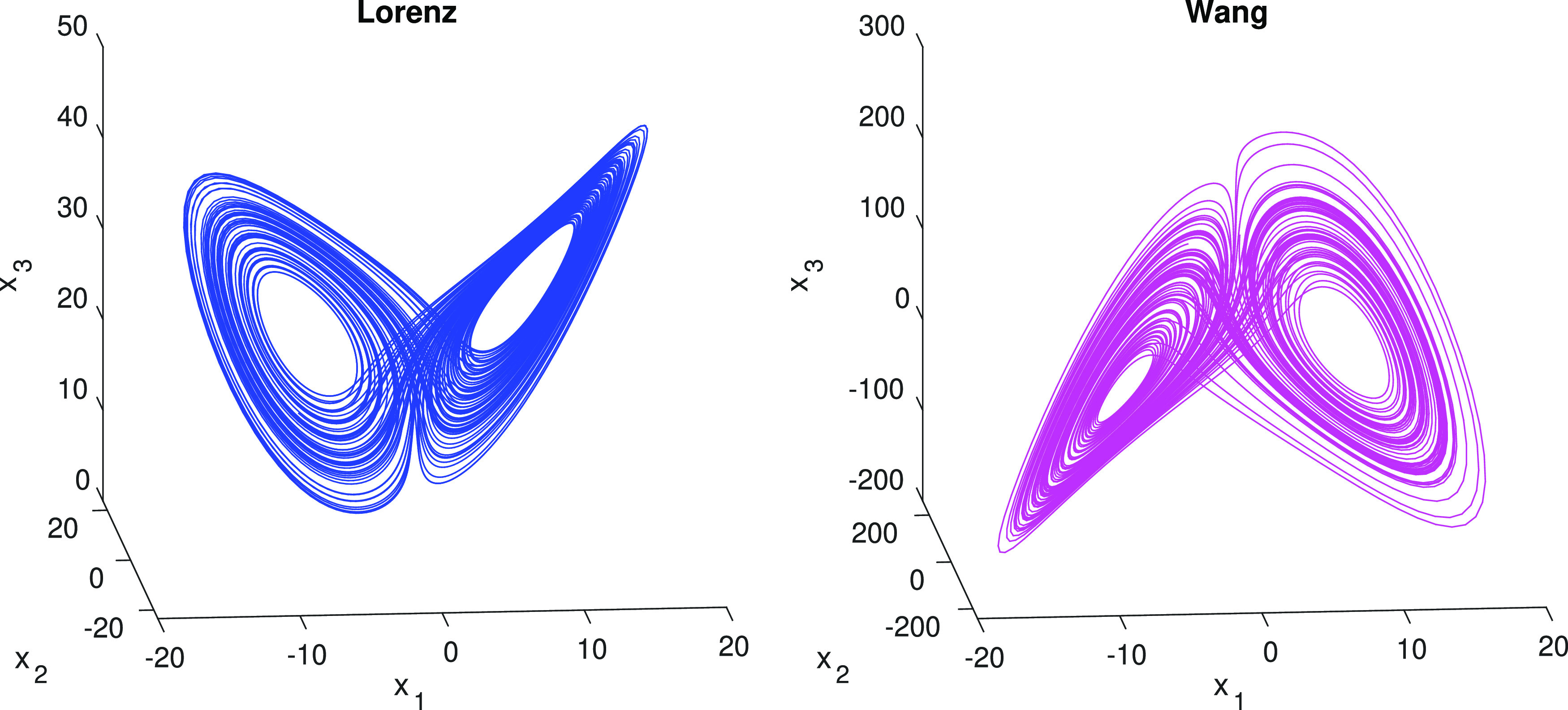
Numerically integrated Lorenz system (13) (blue) and the Wang system Eq. (17) (magenta).

FIG. 2.

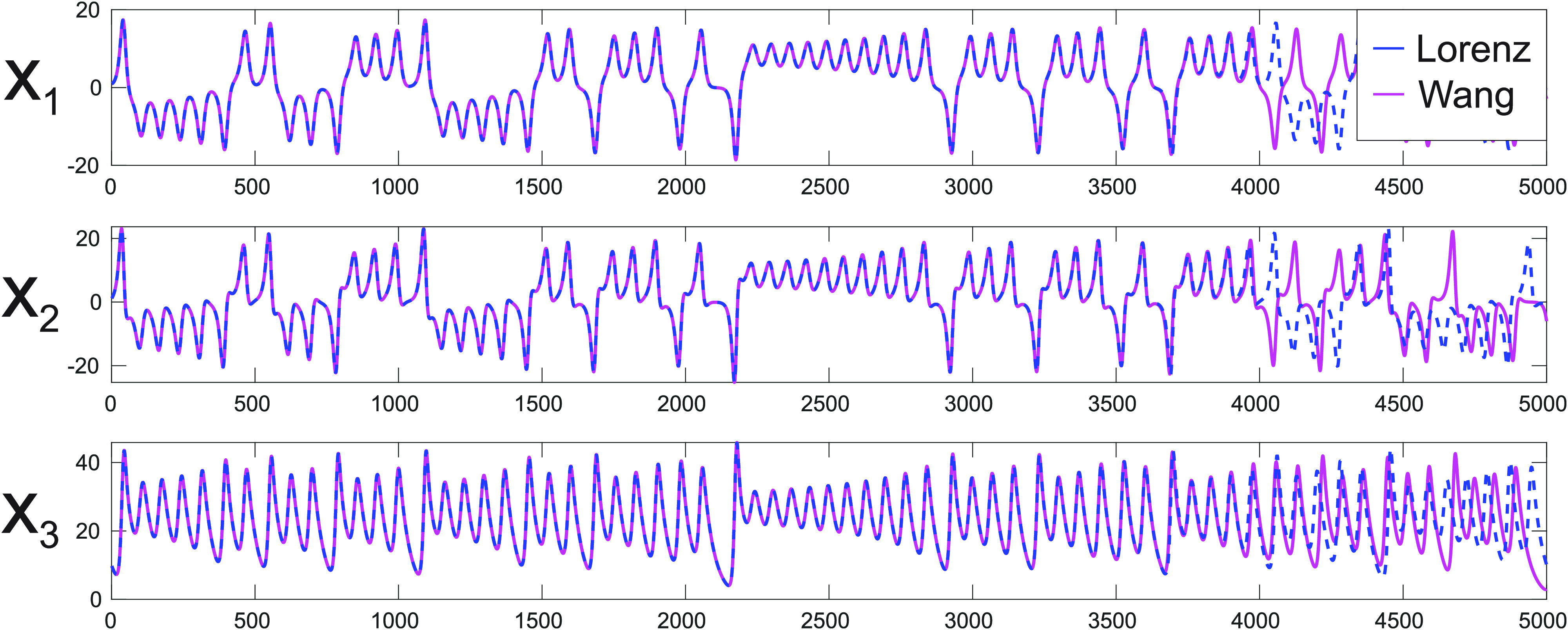
Numerically integrated Lorenz system (13) (blue) and the Wang system Eq. (17) with $a_{8,1,2}=a_{8,2,6}=1$, where we plot $(x_1,\frac{{\displaystyle x_2}}{{\displaystyle \sigma }},R-\frac{x_3}{\sigma })$ in magenta and adjusted initial conditions. The Lyapunov exponents are the same, that is, $(0.906,0,-14.572)$, since there is a transformation between the two systems as required in Ref. 18

B. Systems no.5, no.14 (Lorenz), and no.11

Other interesting examples are systems no.5, no.14 (Lorenz), and no.11. When doing the same procedure as above and attempting to change system no.5 to match the Lorenz system (no.14), we obtain a modified system no.11 as described below. In this case, only two of the time series match when integrated numerically. Going directly from no.5 to no.11, we obtain system no.11 as is.

To align the dynamics of system no.5 in Table I (represented below in a general form) with the Lorenz system [no.14 in Table I or Eq. (13)],

$$\begin{array}{c}{\dot{x}}_1=a_{5,1,1}{x}_1+a_{5,1,2}{x}_2,\\ {\dot{x}}_2=a_{5,2,6}{x}_1{x}_3,\\ {\dot{x}}_3=a_{5,3,0}+a_{5,3,3}{x}_3+a_{5,3,4}{x}_1^2+a_{5,3,5}{x}_1{x}_2,\end{array}$$ (22)

the coefficients ${\alpha }_i$’s in Eq. (10) need to be the same

$$\begin{array}{c}b\sigma (R-1)=a_{5,1,2}{a}_{5,2,6}{a}_{5,3,0},\\ -\sigma =a_{5,2,6}(a_{5,1,2}{a}_{5,3,4}-a_{5,1,1}{a}_{5,3,5}),\\ -b(\sigma +1)=-a_{5,1,1}{a}_{5,3,3},\\ -1=a_{5,2,6}{a}_{5,3,5},\\ \sigma +1=-a_{5,1,1},\\ -b-\sigma -1=a_{5,1,1}+a_{5,3,3},\\ 1=1.\end{array}$$ (23)

With this solution, system no.5 can be written as

$$\begin{array}{c}{\dot{x}}_1=-(\sigma +1)x_1+a_{5,1,2}{x}_2,\\ {\dot{x}}_2=a_{5,2,6}{x}_1{x}_3,\\ {\dot{x}}_3=\frac{{\displaystyle b(R-1)\sigma }}{{\displaystyle a_{5,1,2}{a}_{5,2,6}}}-b{x}_3+\frac{{\displaystyle 1}}{{\displaystyle a_{5,1,2}{a}_{5,2,6}}}{x}_1^2-\frac{{\displaystyle 1}}{{\displaystyle a_{5,2,6}}}{x}_1{x}_2.\end{array}$$ (24)

Equation (24) then shares the time series of the $x_1$ variable with the Lorenz system. The other variables may be scaled and shifted to those of the Lorenz system. To get a system, where all time series are matched, we replace $x_j$, where $j=2,3$ with $s_j{x}_j+d_j$ and match the fixed points of this scaled (by $s_j$) and displaced (by $d_j$) system with the fixed points of the Lorenz system. The shift and scaling parameters are $s_2=\sigma +1$, $s_3=-\sigma ,d_2=0$, and $d_3=(R-1)\sigma$. This transforms the modified system no.5 into the form of system no.11,

$$\begin{array}{c}{\dot{x}}_1=-(\sigma +1)x_1+(\sigma +1)x_2,\\ {\dot{x}}_2=\frac{{\displaystyle (R-1)\sigma }}{{\displaystyle \sigma +1}}{x}_1-\frac{{\displaystyle \sigma }}{{\displaystyle \sigma +1}}{x}_1{x}_3,\\ {\dot{x}}_3=-b{x}_3-\frac{{\displaystyle 1}}{{\displaystyle \sigma }}{x}_1^2+\frac{{\displaystyle (\sigma +1)}}{{\displaystyle \sigma }}{x}_1{x}_2.\end{array}$$ (25)

Figure 3 shows the time series of the original Lorenz system (13) in blue and system (25) in magenta. While $x_1$ and $x_3$ are the same (up to numerical errors), $x_2$ is slightly different. In fact, plotting $\frac{{\displaystyle (\sigma +1)x_2-x_1}}{{\displaystyle \sigma }}$ instead of $x_2$ would make the lines overlap and consequently applying the transformation $x_2\to \frac{{\displaystyle \sigma x_2+x_1}}{{\displaystyle \sigma +1}}$ changes Eq. (25) back to the original Lorenz system. Note that Eq. (24), which is system no.5 in Table I and Eq. (25), which is system no.11 in Table I, and the original Lorenz system shares the same time series of the $x_1$ variable. Numerically, this is not always true. If we integrate system (25) and the Lorenz system (13) with equal values for the initial conditions for the $x_1$ and $x_2$ variables, we get Fig. 3 (integration step size is $\delta t=0.001$ and $\sigma =10$, $R=28$, and $b=\frac{8}{3}$). In this case, all three time series match for a long time, then they depart from each other due to finite number lengths on computers. For other initial conditions, they depart sooner. In theory, $x_1(t)$ should be the same forever.

FIG. 3.

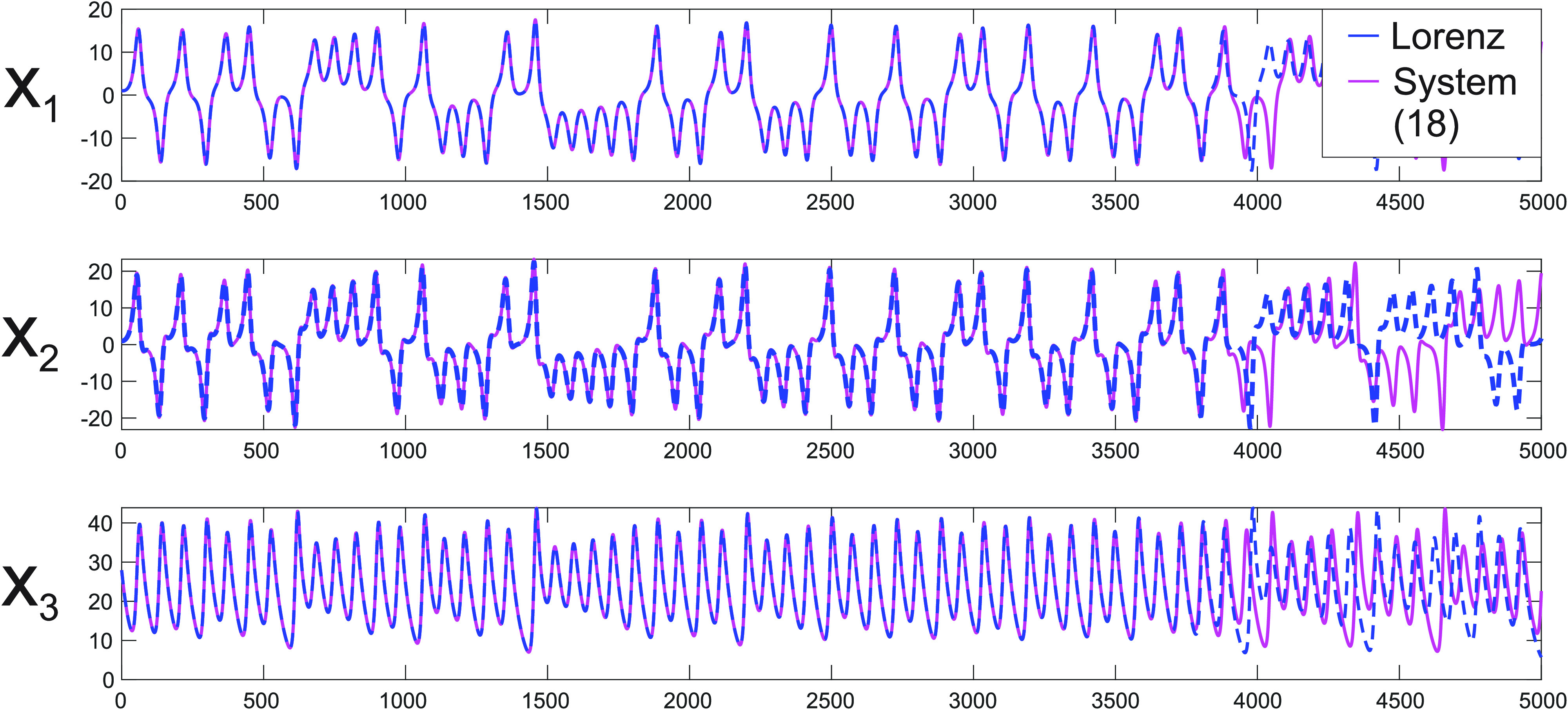
Numerically integrated $(x_1,\frac{{\displaystyle x_2}}{{\displaystyle \sigma }},R-\frac{x_3}{\sigma })$ for the Lorenz system (13) (blue) and system (25) (magenta). The Lyapunov exponents are the same, that is, $(0.906,0,-14.572)$, since there is a transformation between the two systems as required in Ref. 18.

C. System no.6

System no.6

$$\begin{array}{c}{\dot{x}}_1=a_{6,1,1}{x}_1+a_{6,1,2}{x}_2,\\ {\dot{x}}_2=a_{6,2,2}{x}_2+a_{6,2,6}{x}_1{x}_3,\\ {\dot{x}}_3=a_{6,3,3}{x}_3+a_{6,3,5}{x}_1{x}_2\end{array}$$ (26)

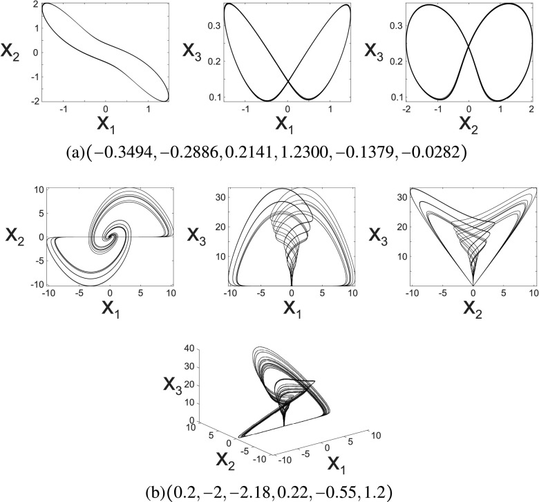
is a Lorenz-like system with a very interesting and different dynamics, as shown in Fig. 4. Although the jerk structure is the same, no single set of coefficients can make the jerk equation of System no.6 equivalent to that of another Lorenz-like system, making System no.6, a unique type of system.

FIG. 4.

System no.6 with two choices for the parameters $(a_{6,1,1},a_{6,1,2},a_{6,2,1},a_{6,2,6},a_{6,3,0},a_{6,3,3},a_{6,3,5})$. (a) $(-0.3494,-0.2886,0.2141,1.2300,-0.1379,-0.0282)$ and (b) $(0.2,-2,-2.18,0.22,-0.55,1.2)$.

IV. NECESSARY CONDITION FOR DIFFEOMORPHISMS TO PRESERVE THE JERK FORM

In this section, a necessary condition for a diffeomorphism to preserve the jerk of a vector field is demonstrated.

Theorem 1

Let $f(\mathbf{x})$ a differentiable vector field in ${\mathbb{R}}^3$, $\mathbf{x}=(x_1,x_2,x_3)$, and $\mathrm{\Phi }:{\mathbb{R}}^3\to {\mathbb{R}}^3$, a local diffeomorphism around ${\mathbf{x}}_{\mathbf{0}}\in {\mathbb{R}}^3$. If

$$\mathrm{\Phi }(\mathbf{x})=({\phi }_1(\mathbf{x}),{\phi }_2(\mathbf{x}),{\phi }_3(\mathbf{x}))$$ (27)

and ${\phi }_j(\mathbf{x})=x_i$ for some $i,j$, then the jerk equation in relation to $x_i$ of

$$\dot{\mathbf{x}}=\mathbf{f}(\mathbf{x})=(f_1(\mathbf{x}),f_2(\mathbf{x}),f_3(\mathbf{x}))$$ (28)

and of the system transformed under $\mathrm{\Phi }$ is the same.

Remark 1

In Theorem 1, ${\phi }_j(\mathbf{x})=x_i$ denotes that at least one of the coordinate functions of $\mathrm{\Phi }(\mathbf{x})$ and must be a projection. Note that ${\phi }_1(\mathbf{x})=h(\mathbf{x})=x_1$ in Sec. II.

Proof.

Without loss of generality, we can consider ${\phi }_i(\mathbf{x})=x_i$. If ${\phi }_j(\mathbf{x})=x_i$, with $i\ne j$, the coordinates’ change given by

$$\{\begin{array}{l}{\psi }_k={\phi }_k,\text{if}k\ne i\text{or}k\ne j,\\ {\psi }_j={\phi }_i,\\ {\psi }_i={\phi }_j\end{array}$$

is such that ${\psi }_i(\mathbf{x})=x_i$. For $i=1$, we define the transformation $\mathrm{\Xi }:{\mathbb{R}}^3\to {\mathbb{R}}^3$ given by

$$\mathrm{\Xi }(\mathbf{x})=(X(\mathbf{x}),Y(\mathbf{x}),Z(\mathbf{x}))$$

with

$$\{\begin{array}{l}X=x_1,\\ Y=L_{\mathbf{f}}X=L_{\mathbf{f}}{x}_1=f_1(\mathbf{x}),\\ Z=L_{\mathbf{f}}^{2}X=L_{\mathbf{f}}Y=\mathrm{\nabla }{f}_1\left(\mathbf{x}\right)\cdot \mathbf{f}{(\mathbf{x})}^{\mathrm{\top }}=\mathrm{\nabla }Y\cdot \mathbf{f}{(\mathbf{x})}^{\mathrm{\top }},\end{array}$$ (29)

where $L_{\mathbf{f}}(\cdot )$ is the Lie derivative of a real function defined by Eq. (2). In order to find the jerk equation of system (28), it is necessary to take the derivative of $\mathrm{\Xi }$ in relation to time as shown in Eq. (30),

$$\{\begin{array}{ll}\dot{X}=& {\dot{x}}_1=f_1(\mathbf{x})=Y,\\ \dot{Y}=& \mathrm{\nabla }Y\cdot \mathbf{f}{(\mathbf{x})}^{\mathrm{\top }}=Z,\\ \dot{Z}=& \mathbf{f}(\mathbf{x})\cdot H_{f_1}\cdot \mathbf{f}{(\mathbf{x})}^{\mathrm{\top }}+\mathrm{\nabla }{f}_1(\mathbf{x})\cdot \mathrm{d}\mathbf{f}(\mathbf{x})\cdot \mathbf{f}{(\mathbf{x})}^{\mathrm{\top }},\end{array}$$ (30)

where $\mathrm{d}\mathbf{f}(\mathbf{x})=\left[\frac{\mathrm{\partial }{f}_i}{\mathrm{\partial }{x}_j}\right]$ is the Jacobian matrix of $\mathbf{f}(\mathbf{x})$ and $H_{f_1}=\left[\frac{{\mathrm{\partial }}^2{f}_1}{\mathrm{\partial }{x}_i\mathrm{\partial }{x}_j}\right]$ is the Hessian of $f_1(\mathbf{x})$ for $i,j=1,2,3$. Now consider a diffeomorphism $\mathrm{\Phi }:{\mathbb{R}}^3\to {\mathbb{R}}^3$ around ${\mathbf{x}}_{\mathbf{0}}\in {\mathbb{R}}^3$ such that ${\phi }_1(\mathbf{x})=x_1$. In the coordinate system $\mathbf{w}=({\phi }_1,{\phi }_2,{\phi }_3)$, the differential Eq. (28) around $\mathrm{\Phi }({\mathbf{x}}_{\mathbf{0}})$ is given by

$$\dot{\mathbf{w}}=\mathrm{d}\mathrm{\Phi }(\mathbf{x})\cdot \mathbf{f}{({\mathrm{\Phi }}^{-1}(\mathbf{w}))}^{\mathrm{\top }}=\hat{\mathbf{f}}{(\mathbf{w})}^{\mathrm{\top }},$$ (31)

where $\mathrm{d}\mathrm{\Phi }$, the Jacobian matrix of $\mathrm{\Phi }$, is given by

$$\mathrm{d}\mathrm{\Phi }=\left[\begin{array}{ccc}1& 0& 0\\ {\displaystyle \frac{\mathrm{\partial }{\phi }_2}{\mathrm{\partial }{x}_1}}& {\displaystyle \frac{\mathrm{\partial }{\phi }_2}{\mathrm{\partial }{x}_2}}& {\displaystyle \frac{\mathrm{\partial }{\phi }_2}{\mathrm{\partial }{x}_3}}\\ {\displaystyle \frac{\mathrm{\partial }{\phi }_3}{\mathrm{\partial }{x}_1}}& {\displaystyle \frac{\mathrm{\partial }{\phi }_3}{\mathrm{\partial }{x}_2}}& {\displaystyle \frac{\mathrm{\partial }{\phi }_3}{\mathrm{\partial }{x}_3}}\end{array}\right].$$ (32)

Consider yet again another transformation $\tilde{\mathrm{\Xi }}:{\mathbb{R}}^3\to {\mathbb{R}}^3$

$$\tilde{\mathrm{\Xi }}(\mathbf{w})=(\tilde{X}(\mathbf{w}),\tilde{Y}(\mathbf{w}),\tilde{Z}(\mathbf{w})),$$

such that

$$\{\begin{array}{ll}\tilde{X}& ={\phi }_1,\\ \tilde{Y}& =L_{\hat{\mathbf{f}}}{\phi }_1=L_{\hat{\mathbf{f}}}\tilde{X},\\ \tilde{Z}& =L_{\hat{\mathbf{f}}}^2{\phi }_1=L_{\hat{\mathbf{f}}}\tilde{Y}.\end{array}$$ (33)

From Eqs. (31) and (32), the first coordinate of $\hat{\mathbf{f}}(\mathbf{w})$ is $f_1({\mathrm{\Phi }}^{-1}(\mathbf{w}))$. Hence,

$$\tilde{Y}=f_1({\mathrm{\Phi }}^{-1}(\mathbf{w}))\text{and}\tilde{Z}=\mathrm{\nabla }{f}_1({\mathrm{\Phi }}^{-1}(\mathbf{w}))\cdot \mathbf{f}{({\mathrm{\Phi }}^{-1}(\mathbf{w}))}^{\mathrm{\top }}.$$

Follow the same steps in the process of obtaining the jerk equation as conducted for transformation $\mathrm{\Xi }(\mathbf{x})$, that is, take the derivative of Eq. (33) in relation to time and get

$$\begin{array}{r}\begin{array}{c}\dot{\tilde{X}}={\dot{\phi }}_1=f_1({\mathrm{\Phi }}^{-1}(\mathbf{w}))=\tilde{Y},\\ \dot{\tilde{Y}}=\mathrm{\nabla }{f}_1({\mathrm{\Phi }}^{-1}(\mathbf{w}))\cdot \mathrm{d}{\mathrm{\Phi }}^{-1}\cdot {\dot{\mathbf{w}}}^{\mathrm{\top }}\\ =\mathrm{\nabla }{f}_1({\mathrm{\Phi }}^{-1}(\mathbf{w}))\cdot \mathrm{d}{\mathrm{\Phi }}^{-1}\cdot \hat{\mathbf{f}}{(\mathbf{w})}^{\mathrm{\top }}\\ =\mathrm{\nabla }{f}_1({\mathrm{\Phi }}^{-1}(\mathbf{w}))\cdot \mathbf{f}{({\mathrm{\Phi }}^{-1}(\mathbf{w}))}^{\mathrm{\top }}=\tilde{Z},\\ \dot{\tilde{Z}}=\underset{{(\mathrm{d}{\mathrm{\Phi }}^{-1}\cdot \hat{\mathbf{f}}{(\mathbf{w})}^{\mathrm{\top }})}^{\mathrm{\top }}}{\underbrace{\hat{\mathbf{f}}(\mathbf{w})\cdot {(\mathrm{d}{\mathrm{\Phi }}^{-1})}^{\mathrm{\top }}}}\cdot H_{f_1}({\mathrm{\Phi }}^{-1}(\mathbf{w}))\cdot \mathrm{d}{\mathrm{\Phi }}^{-1}\cdot \hat{\mathbf{f}}{(\mathbf{w})}^{\mathrm{\top }}\\ +\mathrm{\nabla }{f}_1({\mathrm{\Phi }}^{-1}(\mathbf{w}))\cdot \mathrm{d}\mathbf{f}({\mathrm{\Phi }}^{-1}(\mathbf{w}))\cdot \mathrm{d}{\mathrm{\Phi }}^{-1}\cdot \hat{\mathbf{f}}(\mathbf{w}).\end{array}\end{array}$$

From Eq. (31) and ${\mathrm{\Phi }}^{-1}(\mathbf{w})=\mathbf{x}$, for every $\mathbf{x}$ around ${\mathbf{x}}_{\mathbf{0}}$ then,

$$\dot{\tilde{Z}}=\mathbf{f}(\mathbf{x})\cdot H_{f_1}(\mathbf{x})\cdot \mathbf{f}{(\mathbf{x})}^{\mathrm{\top }}+\mathrm{\nabla }{f}_1(\mathbf{x})\cdot \mathrm{d}\mathbf{f}(\mathbf{x})\cdot f{(\mathbf{x})}^{\mathrm{\top }}.$$ (34)

The right-hand side of equation $\dot{\tilde{Z}}$ in (34), the jerk equation for the transformed system, is exactly the same as the right-hand of equation $\dot{Z}$ in Eq. (30), which completes the proof for $i=1$. For $i=2,3$, the proof can be obtained using the same steps.

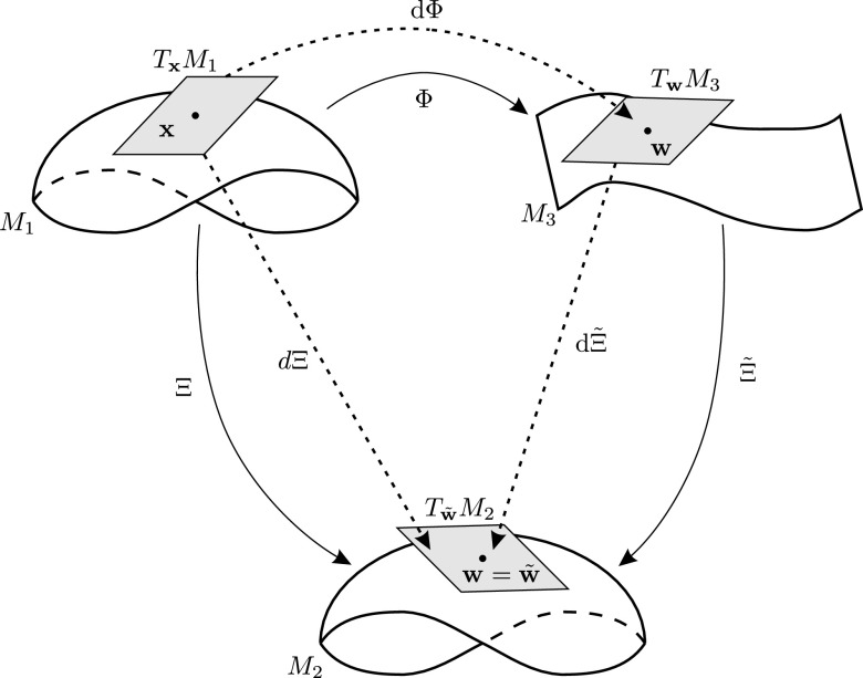
The transformation can be summarized in Fig. 5.

FIG. 5.

Diagram of $\mathbf{x}\stackrel{\mathrm{\Phi }}{⟶}\mathbf{w}\stackrel{\tilde{\mathrm{\Xi }}}{⟶}\tilde{\mathbf{w}}\stackrel{{\mathrm{\Xi }}^{-1}}{⟶}\mathbf{x}$.

V. TRANSFORMATION THAT LEADS TO COEXISTING ATTRACTORS

We further investigate the role of fixed points, stability issues, and pitfalls of the numerical analysis of dynamical systems reconstructed from a single time series. Max Planck’s idea of “natural units”¹⁹ illustrate the fact that a system’s behavior can be described in a simple or more complicated way depending on the coordinate system. We present an example of the Lorenz system¹⁴ and a modified Lorenz system that was obtained by coordinate transformations of the unobserved variables. Both systems have the same differential model and share the same time series of $x_1(t)$, but the number of fixed points can change and lead to coexisting attractors. Let us consider the Lorenz system (13) with variables $(x_1,x_2,x_3)$ and the system

$$\begin{array}{c}{\dot{y}}_1=\sigma (-y_1+\frac{{\displaystyle y_2}}{{\displaystyle y_3}}),\\ {\dot{y}}_2=\frac{{\displaystyle -y_2{y}_3(y_3+b(y_2^2+y_3))+y_1((R-y_3)y_3^3-y_2^2(y_3^3-1))}}{{\displaystyle y_3(2y_2^2+y_3)}},\\ \\ {\dot{y}}_3=\frac{{\displaystyle -y_3((b-2)y_2^2+b{y}_3)+y_1{y}_2(1-2R{y}_3^2+2y_2^2{y}_3^2+2y_3^3)}}{{\displaystyle 2y_2^2+y_3}}.\end{array}$$ (35)

System (35) was obtained by the transformation $x_1\to x_1$, $x_2\to \frac{{\displaystyle x_2}}{{\displaystyle x_3}}$, and $x_3\to x_3+x_2^2$, or

$$\begin{array}{c}{x}_1=y_1,\\ x_2=\frac{{\displaystyle y_2}}{{\displaystyle y_3}},\\ x_3=y_3+y_2^2\end{array}$$ (36)

from the original Lorenz system. $x_3=0$ would make the Lorenz system 2D and is, therefore, not allowed. Additionally, $(x_1,x_2,x_3)=(0,0,0)$ is an unstable fixed point. Therefore, this transformation does not cause any singularities. According to Theorem 1 in Sec. IV, both systems generate the same time series $x_1(t)=y_1(t)$. To numerically obtain the attractor of system (35), we can (i) directly integrate this system or (ii) we can integrate the Lorenz system and apply the inverted transformation (36),

$$\begin{array}{c}{y}_1=x_1,\\ y_{2_{1,2}}=\frac{{\displaystyle -1\pm \sqrt{1+4x_2^2{x}_3}}}{{\displaystyle 2x_2}},\\ y_{3_{1,2}}=\frac{{\displaystyle -1\pm \sqrt{1+4x_2^2{x}_3}}}{{\displaystyle 2x_2^2}}\end{array}$$ (37)

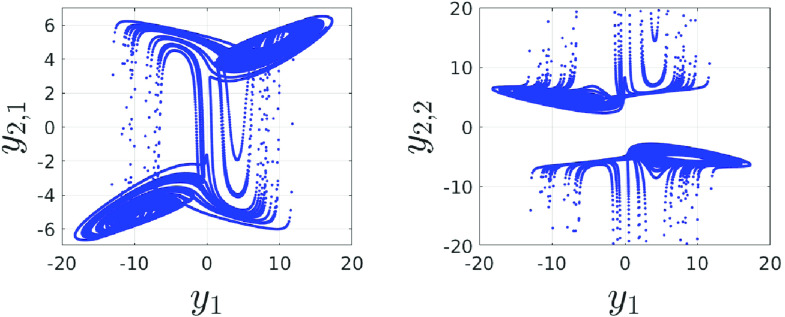
to those numerical values. Both plots should be the same. Figure 6 shows (i) and Fig. 7 shows the coexisting attractors (ii). The left plot in Fig. 7 is similar to the left plot in Fig. 6. The right plot can only be obtained by plotting $(y_1,y_{2_2})$. Numerically, this is not possible because of $y_{2_2}\to \pm \mathrm{\infty }$.

FIG. 6.

Phase-portraits of the modified Lorenz system (35).

FIG. 7.

Phase-portraits of the numerically integrated Lorenz system with the transformation (37).

The attractor of System (35) shown in Fig. 6 has four fixed points,

$$\begin{array}{rl}{\mathit{\xi }}_{1,2}& =(\sqrt{b(R-1)},\frac{-1\pm \sqrt{1+4b{(R-1)}^2}}{2\sqrt{b(R-1)}},\\ & \frac{-1\pm \sqrt{1+4b{(R-1)}^2}}{2(b(R-1))}),\\ \\ {\mathit{\xi }}_{3,4}& =(-\sqrt{b(R-1)},\frac{1\pm \sqrt{1+4b{(R-1)}^2}}{2\sqrt{b(R-1)}},\\ & \frac{-1\mp \sqrt{1+4b{(R-1)}^2}}{2(b(R-1))}),\end{array}$$ (38)

while the standard Lorenz system has only three fixed points,

$$\begin{array}{c}{\mathit{\xi }}_1=(0,0,0),\\ {\mathit{\xi }}_{2,3}=(\pm \sqrt{b(R-1)},\pm \sqrt{b(R-1)},R-1).\end{array}$$ (39)

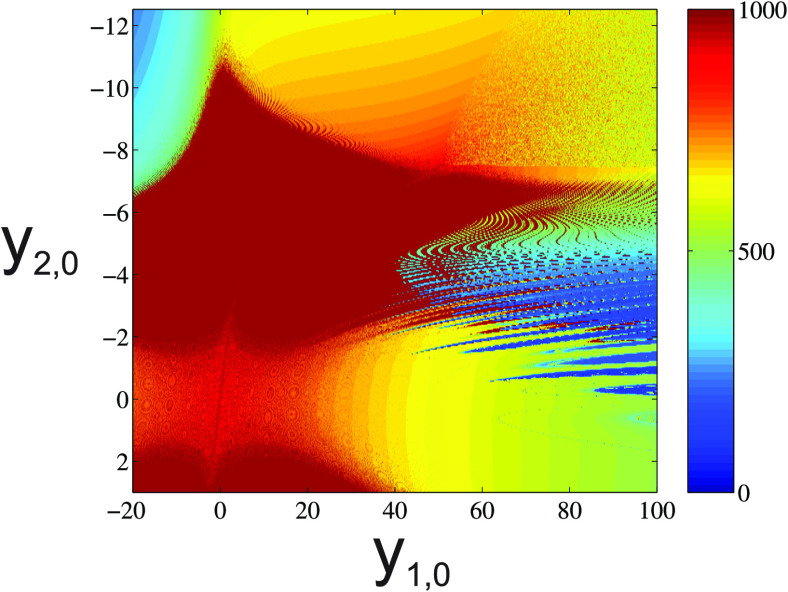
In Fig. 8, the dependence on the initial conditions is illustrated. The initial conditions that determine which of the two coexisting attractors is visited are very close and seem to have a fractal structure. This also causes the numerical instability of the system since numbers during numerical integration only a finite number of digits is processed which represents a small change of the number and can cause a jump from one attractor to the other.

FIG. 8.

Numerical stability in dependence of the initial conditions $y_{1,0}$ and $y_{2,0}$ of system (35). The third initial condition is fixed as $y_{3,0}=1.0113959$. The colors denote the length of the numerical integration before $|y_1|>100$.

System (35), therefore, will be numerically integrated to always give Fig. 6 with the four coexisting fixed points, instead of one of the two attractors with the corresponding two fixed points. The fixed point of the Lorenz system located at the origin is not present in either one of the modified Lorenz attractors since it became singular. The number of fixed points, therefore, cannot be used to validate a system. System (35) can also be interpreted as the Lorenz system in a changed coordinate system determined by the transformation between these two systems. Finally, it is worth noting that the two systems share the same Lyapunov exponents since the transformation between them meets the mild assumptions given in Ref. 18.

VI. CONCLUSION

In this paper, we investigated the connections and transformations between 17 Lorenz-like systems that were introduced in Ref. 11. We showed which systems can share the same time series and transformations between systems. We also proved that transformations of the unobserved variables do not change the jerk form and showed an example of how such a transformation can change the systems behavior and lead to coexisting attractors. Finally, we demonstrated that sharing of the same jerk form by another model, derived from the study of a different phenomenon in another domain, can provide insights into behaviors in that other domain.

SUPPLEMENTARY MATERIAL

In the supplementary material, we present the calculation results for the Lyapunov exponents of the Lorenz and the Wang systems discussed in the paper. While there is a comprehensive mathematical proof ensuring that the Lyapunov exponents remain consistent across systems that can be mutually transformed, we provide a brief proof for the case of linear transformations.

AUTHOR DECLARATIONS

Conflict of Interest

The authors have no conflicts to disclose.

Authors Contribution

Claudia Lainscsek and Eduardo M. A. M. Mendes contributed equally to this paper.

Claudia Lainscsek: Conceptualization (lead); Formal analysis (lead); Investigation (lead); Methodology (lead); Software (lead); Validation (lead); Visualization (lead); Writing – original draft (lead); Writing – review & editing (lead). Eduardo M. A. M. Mendes: Conceptualization (lead); Formal analysis (lead); Funding acquisition (equal); Investigation (lead); Methodology (lead); Software (lead); Validation (lead); Visualization (lead); Writing – original draft (lead); Writing – review & editing (lead). Gustavo H. O. Salgado: Formal analysis (equal); Investigation (equal); Methodology (equal); Writing – original draft (equal); Writing – review & editing (equal). Terrence J. Sejnowski: Conceptualization (supporting); Formal analysis (supporting); Funding acquisition (lead); Investigation (supporting); Methodology (supporting); Resources (lead); Writing – original draft (supporting); Writing – review & editing (equal).

Author Contributions

Claudia Lainscsek: Conceptualization (lead); Formal analysis (lead); Investigation (lead); Methodology (lead); Software (lead); Validation (lead); Visualization (lead); Writing – original draft (lead); Writing – review & editing (lead). Eduardo M. A. M. Mendes: Conceptualization (lead); Formal analysis (lead); Funding acquisition (equal); Investigation (lead); Methodology (lead); Software (lead); Validation (lead); Visualization (lead); Writing – original draft (lead); Writing – review & editing (lead). Gustavo H. O. Salgado: Formal analysis (equal); Investigation (equal); Methodology (equal); Writing – original draft (equal); Writing – review & editing (equal). Terrence J. Sejnowski: Conceptualization (supporting); Formal analysis (supporting); Funding acquisition (lead); Investigation (supporting); Methodology (supporting); Resources (lead); Writing – original draft (supporting); Writing – review & editing (equal).

DATA AVAILABILITY

All the data used in this work were produced with basic codes for integrating the systems under study by using a Runge–Kutta integration scheme found in Ref. 20.

REFERENCES

- 1.Lainscsek C., “Nonuniqueness of global modeling and time scaling,” Phys. Rev. E 84, 046205 (2011). 10.1103/PhysRevE.84.046205 [DOI] [PubMed] [Google Scholar]
- 2.Takens F., “Detecting strange attractors in turbulence,” in Dynamical Systems and Turbulence, Warwick 1980, Lecture Notes in Mathematics Vol. 898, edited by D. A. Rand and L.-S. Young (Springer, Berlin, 1981).
- 3.Packard N. H., Crutchfield J. P., Farmer J. D., and Shaw R. S., “Geometry from a time series,” Phys. Rev. Lett. 45, 712 (1980). 10.1103/PhysRevLett.45.712 [DOI] [Google Scholar]
- 4.Sauer T., Yorke J. A., and Casdagli M., “Embedology,” J. Stat. Phys. 65, 579 (1991). 10.1007/BF01053745 [DOI] [Google Scholar]
- 5.Crutchfield J. and McNamara B., “Equations of motion from a data series,” Complex Syst. 1(3), 417–452 (1987); ISSN: 0891-2513. [Google Scholar]
- 6.Broomhead D. and King G., “Extracting qualitative dynamics from experimental data,” Phys. D 20, 217 (1986). 10.1016/0167-2789(86)90031-X [DOI] [Google Scholar]
- 7.Gibson J. F., Farmer J. D., Casdagli M., and Eubank S., “An analytic approach to practical state space reconstruction,” Phys. D 57, 1 (1992). 10.1016/0167-2789(92)90085-2 [DOI] [Google Scholar]
- 8.Gouesbet G., “Reconstruction of the vector fields of continuous dynamical systems from numerical scalar time series,” Phys. Rev. A 43(10), 5321–5331 (1991). 10.1103/PhysRevA.43.5321 [DOI] [PubMed] [Google Scholar]
- 9.Gouesbet G., “Reconstruction of vector fields: The case of the Lorenz system,” Phys. Rev. A 46(4), 1784–1796 (1992). 10.1103/PhysRevA.46.1784 [DOI] [PubMed] [Google Scholar]
- 10.Aguirre L. and Letellier C., “Modeling nonlinear dynamics and chaos: A review,” Math. Prob. Eng. 2009, 238960 (2009). 10.1155/2009/238960 [DOI] [Google Scholar]
- 11.Lainscsek C., “A class of Lorenz-like systems,” Chaos 22, 013126 (2012). 10.1063/1.3689438 [DOI] [PubMed] [Google Scholar]
- 12.Malasoma J. M., “What is the simplest dissipative chaotic Jerk equation which is parity invariant?,” Phys. Lett. A 264(5), 383–389 (2000). 10.1016/S0375-9601(99)00819-1 [DOI] [Google Scholar]
- 13.Mendes E. M. A. M., Lainscsek C., and Letellier C., “Diffeomorphical equivalence vs topological equivalence among Sprott systems,” Chaos 31(8), 083126 (2021). 10.1063/5.0058330 [DOI] [PubMed] [Google Scholar]
- 14.Lorenz E. N., “Deterministic nonperiodic flow,” J. Atmos. Sci. 20, 130–141 (1963). [DOI] [Google Scholar]
- 15.Gouesbet G. and Letellier C., “Global vector-field reconstruction by using a multivariate polynomial approximation on nets,” Phys. Rev. E 49, 4955 (1994). 10.1103/PhysRevE.49.4955 [DOI] [PubMed] [Google Scholar]
- 16.Wang Y., Singer J., and Bau H., “Controlling chaos in a thermal convection loop,” J. Fluid Mech. 237, 479–498 (1992). 10.1017/S0022112092003501 [DOI] [Google Scholar]
- 17.Chen G. and Ueta T., “Yet another chaotic attractor,” Int. J. Bifurcat. Chaos 9(7), 1465 (1999). 10.1142/S0218127499001024 [DOI] [Google Scholar]
- 18.Eichhorn R., Linz S. J., and Hänggi P., “Transformation invariance of Lyapunov exponents,” Chaos, Solitons Fractals 12(8), 1377–1383 (2001). 10.1016/S0960-0779(00)00120-X [DOI] [Google Scholar]
- 19.Planck M., “Über irreversible Strahlungsvorgänge,” Ann. Phys. 306(1), 69–122 (1900). [Google Scholar]
- 20.Press W., Flannery B., Teukolsky S., and Vetterling W., Numerical Recipes in C (Cambridge University Press, New York, 1990). [Google Scholar]
Associated Data
This section collects any data citations, data availability statements, or supplementary materials included in this article.
Supplementary Materials