Abstract
In this work, we propose a novel deep learning reconstruction framework for rapid and accurate reconstruction of 4D flow MRI data. Reconstruction is performed on a slice-by-slice basis by reducing artifacts in zero-filled reconstructed complex images obtained from undersampled k-space. A deep residual attention network FlowRAU-Net is proposed, trained separately for each encoding direction with 2D complex image slices extracted from complex 4D images at each temporal frame and slice position. The network was trained and tested on 4D flow MRI data of aortic valvular flow in 18 human subjects. Performance of the reconstructions was measured in terms of image quality, 3-D velocity vector accuracy, and accuracy in hemodynamic parameters. Reconstruction performance was measured for three different k-space undersamplings and compared with one state of the art compressed sensing reconstruction method and three deep learning-based reconstruction methods. The proposed method outperforms state of the art methods in all performance measures for all three different k-space undersamplings. Hemodynamic parameters such as blood flow rate and peak velocity from the proposed technique show good agreement with reference flow parameters. Visualization of the reconstructed image and velocity magnitude also shows excellent agreement with the fully sampled reference dataset. Moreover, the proposed method is computationally fast. Total 4D flow data (including all slices in space and time) for a subject can be reconstructed in 69 seconds on a single GPU. Although the proposed method has been applied to 4D flow MRI of aortic valvular flows, given a sufficient number of training samples, it should be applicable to other arterial flows.
Keywords: 4D flow MRI, Aortic Flow, Deep Residual Network, Hemodynamics, Deep Learning
I. Introduction
Hemodynamic parameters such as blood flow rate, peak velocity, pressure are widely used clinically to make important decisions about diagnosis, prognosis, and therapy in cardiovascular disease. 4D phase contrast (PC) MRI or 4D flow MRI is a non-invasive method that provides time-resolved three-dimensional blood velocity fields in a 3-D volume from which hemodynamic parameters can be calculated. In PC MRI, the velocity of blood is encoded in the phase of MR signal. Moving spins accumulate an extra phase offset in a spatially varying magnetic field, with the phase offset being proportional to velocity in the direction of the applied gradient. Flow encoding gradients can be applied to two or more axes. By measuring the phase shift of moving spins, velocity along each axis can be measured. In 4D flow MRI, velocity-sensitive flow encoding gradient is applied in three directions, which provides three different velocity components with time and corresponding 3-dimensional anatomic coverage. However, data acquisition in k-space along three different directions with time makes the 4D flow acquisition very lengthy. It is also important to maintain good spatial and temporal resolution during acquisition to accurately compute hemodynamic parameters. In 4D flow MRI, a trade-off between scan time and resolution occurs due to the higher dimensional acquisition. To reduce scan time, in the past, various methods have been proposed. These include parallel MRI such as SENSE [33] and GRAPPA [32], non-Cartesian trajectory acquisitions, namely radial or spiral acquisitions [4],[5] and Compressed sensing [6],[7],[11] methods. In compressed sensing, scan time is reduced by taking fewer samples in k-space (reduced number of phase-encoding steps), and image is reconstructed from undersampled k-space data by exploiting sparsity in pixel domain or a transform domain. For compressed sensing PC MRI reconstruction, several techniques were proposed to reconstruct magnitude and phase with fidelity from undersampled k-space. In [9], a separate magnitude and phase regularization method is proposed, and a regularizer function is introduced, which is periodic in phase and accommodates phase wrap. Another method is proposed in [10], which exploits the sparsity of complex difference images and minimizes the total variation (TV) of both encoded and compensated images. A 4D flow imaging approach is proposed in [11], where temporal and spatial sparsity is exploited in the wavelet domain by an empirical Bayesian method. Minimization of sparsity by L1 minimization can be computationally expensive. Despite impressive acceleration factors, achieving clinically relevant reconstruction time remains a challenge for many methods. Though acquisition time decreases in these methods because they only acquire a fraction of k-space, the reconstruction times increase considerably. To minimize reconstruction times, in recent efforts, deep learning with convolutional neural networks (CNN) has been applied to different medical imaging modalities. Not only reduced reconstruction times but also Deep CNN architecture’s ability to identify intricate features from data has shown better reconstruction results than the state-of-the-art methods. End to end mapping from subsampled k-space or zero-filled images to fully sampled images were proposed in several studies. In [12], a deep cascade of CNNs is proposed, which reconstructs a cine sequence of 2D cardiac MR images within a second. The proposed architecture took input images from undersampled cartesian acquired data and combined convolution and data sharing approaches to learn spatio-temporal relation in a cine sequence. [13] proposed a region of interest-based approach ROIRecNet where a deep neural network based on cascaded CNNs is used to interpolate missing k-space values followed by a U-net which segmented the ROI to focus reconstruction on a region of interest. An image domain-based reconstruction approach by U-net is proposed in [14], which reconstructs brain MR images by reducing artifact from the zero-filled reconstructed image of 29% undersampled k-space. Another U-net based architecture is proposed in [15] that considers the reconstruction problem as a missing k-space problem and performed complex k-space learning to fill in the missing data. [37] proposed a generative adversarial network (GAN) based network that reduces aliasing artifacts from zero-filled images and preserves texture and edges from 2D brain MRI images.
However, the above-mentioned state of the art deep learning approaches are proposed for applications where magnitude image is of main interest and phase is not relevant. In 4D flow MRI, phase is the quantity of interest. Implementing an end-to-end 4D flow reconstruction by deep learning is challenging because the high dimensional nature of 4D flow makes it difficult to gather enough high-quality data for training. There had not been a previous study on deep learning reconstruction of 4D flow until recently, an approach called FlowVN is proposed [16]. FlowVN is a model-based approach - where 10 steps of iterative reconstruction is performed by an unrolled 3D variational network. This approach is similar in spirit to previously proposed networks involving other MR modalities [17– 19], where prior information or optimal parameters are learned beforehand by a neural network and incorporated into the framework of compressed sensing.
In our recent work [21], we proposed phase contrast image reconstruction from zero-filled reconstructed complex image in one encoding direction using a 2-D U-net architecture. A complex image consists of magnitude and phase, where phase image is the main quantity of interest as blood velocity is encoded in phase. Zero-filled reconstruction corrupts both magnitude and phase by creating artifacts in the image. In [21], we showed that the magnitude and velocity of PC MRI can be restored in a single encoding direction with high fidelity by complex image domain learning using the U-Net. In this paper, we improve on our previous results by adopting a combined residual and attention mechanism in the U-Net and propose an approach for 4D flow reconstruction by extending reconstruction to three velocity encoding directions. We propose an independent reconstruction approach for 4D Flow MRI, a data-driven image domain de-aliasing-based approach. The advantage of this approach is that there is no involvement of k-space in the training process, which is relevant when dealing with images acquired by different sequences or MRI scanners. The proposed approach is more versatile, agnostic to the specific of k-space, and reconstruction is a hassle-free plug-and-play approach once we have the zero-filled reconstructed images from the acquisition. The main contributions of this paper are as follows-
We propose a novel 2-D network architecture where integrated residual block and spatial and channel-wise attention block is used as the backbone of a Unet network. We refer to our proposed network as Flow Residual Attention U-net or FlowRAU-net. Proposed FlowRAU-net reduces artifacts in zero-filled reconstructed complex images and restores velocity information in all encoding directions by learning to map zero-filled reconstructed complex image to fully sampled complex image for each encoding direction separately.
Performance of the reconstruction is measured in terms of reconstructed image quality, 3D velocity vector accuracy from phase image at three encoding directions, and two flow parameters- flow rate and peak velocity. Proposed FlowRAU-net shows improved ability for reconstruction and better performance measures over three state-of-the-art deep learning architectures for reconstruction [21], [37], [38] and compressed sensing dynamic total variation reconstruction [20] method.
Reconstruction time of 4D flow is significantly lower than the state-of-the-art compressed sensing methods (7–8 minutes). Each 2-D complex image can be reconstructed within 150ms by FlowRAU-net, and the total 4D flow data for one subject can be reconstructed within 69 seconds by the proposed 4D flow reconstruction framework.
II. Proposed Method
A. Problem Formulation
In accelerated 4D flow MRI, a fraction of k-space is acquired to accelerate the acquisition, and image reconstruction problem is solved by finding the solution of the inverse problem -
| (1) |
Here u ∈ CN denotes time resolved complex valued 3D image at different velocity encoding direction. u = meip, where m is magnitude image, and p is phase image. N= Nx× Ny× Nz× Nt× Ni where Nx× Ny× Nz is 3D complex image volume and Ni and Nt denotes total number of velocity encodings and number of cardiac phases. y ∈ CM denotes undersampled k-space where M≪N and E denotes system matrix. Direct solution of equation (1) is not possible as system is undetermined for M≪N. Filling the unmeasured k-space with zeros and performing direct inversion creates zero-filled reconstructed complex image uo ∈ CN with artifacts. To accommodate small training data in 4D flow MRI, 2D complex image (Nx× Ny) is extracted from uo at different slice position z and temporal position t and reconstruction is done by learning direct mapping of 2D complex image in uo to 2D complex image in u. The main idea is to train the proposed neural network FlowRAU-net with 2D complex image pair with sufficient past training data so that the network will predict an output image close to the fully sampled image from an unseen zero-filled reconstructed input. The mapping function is learned separately at each velocity encoding as different encoding direction corresponds to different phase orientation and range of velocity. The velocity sensitive encoding is generally performed in foot-head (FH) direction, anterior-posterior (AP) direction, and right-left (RL) direction. Phase image p at each encoding direction contains velocity in that direction, which is the primary quantity of interest in 4D flow MRI. Fig. 1 shows the proposed overall reconstruction framework. Zero-filled reconstruction of subsampled k-space creates complex image uo in the spatial domain. Proposed network FlowRAU-net is trained with 2D complex image extracted from time-resolved 3D volume of uo at each encoding direction separately. FlowRAU-net can reconstruct artifact free 2D complex image containing 2D magnitude and phase for corresponding velocity encoding direction after learning the mapping function. Reconstructed 2D phase image at FH, AP, and RL directions give 3D velocity information, and 2D magnitude image gives corresponding structural information. 2D reconstruction at all slices and time positions at each encoding creates a total complex image domain of 4D flow.
Fig.1:
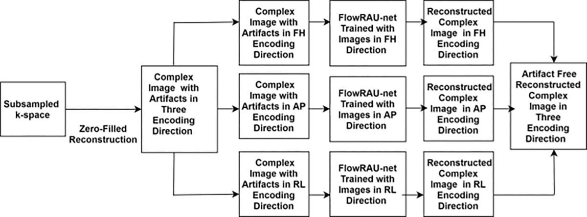
Illustration of proposed reconstruction approach. Zero-filled reconstruction of acquired k-space will create complex images u0 ∈ CN with artifacts. FlowRAU-net is trained separately at each encoding direction by 2D complex image pair from u0 and u. Trained network can reconstruct 2D complex images at three encoding directions separately and produce 3 directional velocity images from the phase. Reconstructed 2D complex images at all slices and time positions at each encoding create total complex image domain of 4D flow.
B. Network Architecture
The proposed network FlowRAU-net is based on a 2D encoder-decoder structure. Encoder-decoder architecture has been one of the most popular frameworks for reconstruction in different imaging modalities as it enables deeper feature extraction in the network. Encoder extracts shallow, and deep features in the network, and decoder retrieves the features by upsampling and concatenation, maintaining the same spatial resolution. Fig. 2(a) shows the overall architecture of FlowRAU-net. The network takes a 2-channel 80× 80 complex image as input where the channel stores real and imaginary parts of zero-filled reconstructed input. A residual block followed by an attention block is proposed as the backbone of an encoder-decoder architecture. From our previous study in [21], reconstruction of phase contrast MRI in through-plane direction using a basic encoder-decoder U-net architecture does not improve accuracy when the number of convolutional layers is increased. An increasing number of layers leads to the gradient vanishing problem and creates difficulty in training the network. In prior work, different segmentation networks [22], [23] have used Resnet as the backbone of encoder-decoder structure to mitigate the vanishing gradient problem. Similarly, herein we adopt a residual block instead of a traditional convolution block. Fig. 2(b) shows the adopted residual block. A single residual block consists of convolution layers, batch normalization, and ReLU activation function. In our proposed method, the number of convolutional layers at each residual block is 3. The convolution block consists of a 3×3 filter with stride 1. The number of filters in the encoder residual block is 64, 128, and 256. After encoder blocks, there is a bottleneck layer consisting of one convolution layer of 512 filters. The bottleneck layer contains the most reduced dimensionality of the input with the most increased depth, which helps in efficient feature map learning. The bottleneck feature vector is then decoded to reconstruct the image in the decoder path. The number of filters in the decoder residual block is the same but in reverse order.
Fig. 2:
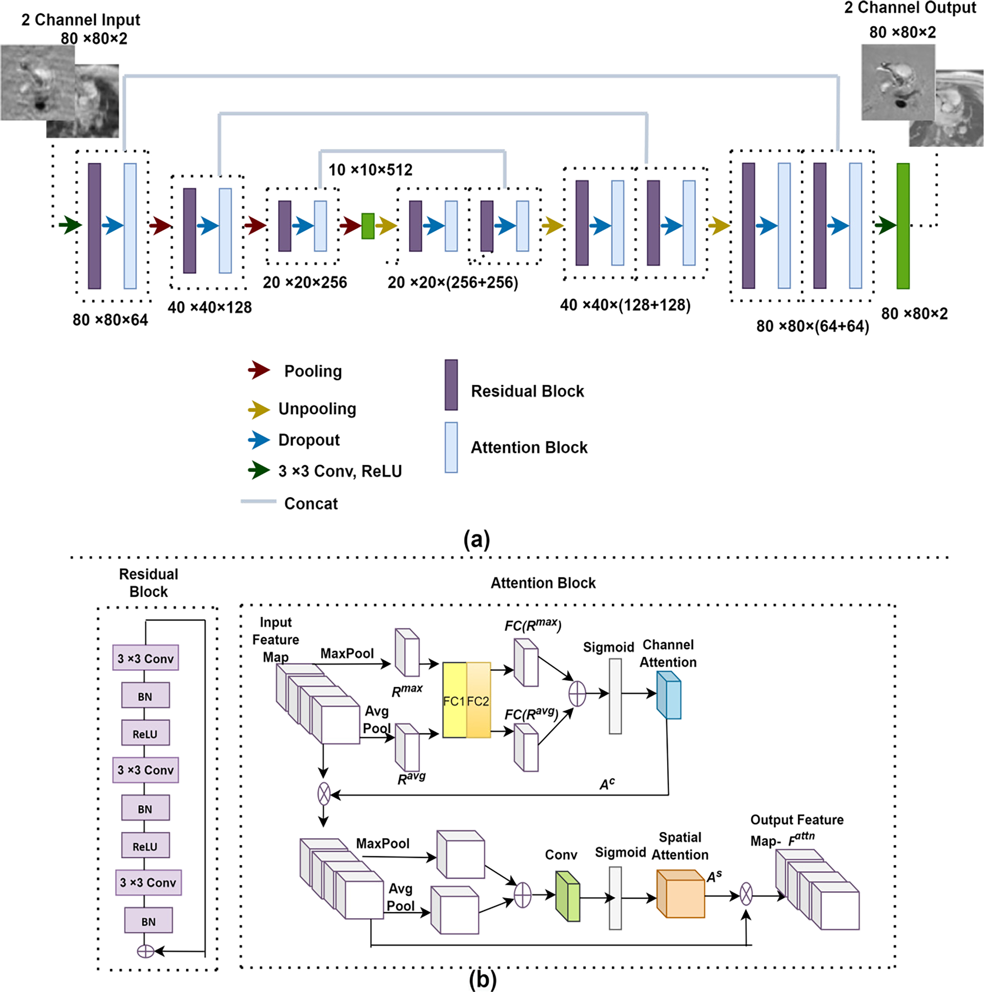
(a) The overall architecture of FlowRAU-net. FlowRAU-net takes a 2-channel 80× 80 image as input where the channel stores real and imaginary part of zero-filled reconstructed input. Back-to-back residual block and attention block is adopted as the backbone of a U-Net. Each residual attention (RA) block is followed by maxpooling in the encoder network and upsampling and concatenation in the decoder network. (b) The architecture of a RA block. Each residual block consists of 3 convolutional layers followed by batch normalization and ReLU. Attention block consists of channel attention and spatial attention.
Though residual block in encoder and decoder improves accuracy, when we go deeper in the CNN, the volume of irrelevant pixel increases in the network, which creates inefficient weight learning. That is why before each pooling layer in the encoder, an attention mechanism is adopted to give significance to important features and ensure efficient pooling of features. Attention is also applied in the decoder path before upsampling and concatenation so that the important features are weighted in later layers. The output features from the residual block go through a dropout layer before entering the attention block for better generalization during training. Residual and attention block together create the residual attention (RA) block. Each RA block is followed by maxpooling in the encoder and average unpooling in the decoder. Average unpooling is followed by a concatenation of encoder feature map maintaining same spatial resolution. After each maxpooling the next RA block consists of the same number of convolutions with an increased number of filters by factor of 2.
Fig. 2(b) describes the attention mechanism in detail. Different state of the art methods [24–28] adopted attention mechanism with CNNs and achieved better results in several applications like segmentation and classification. [38] and [41] adopted an attention mechanism in reconstruction application. [38] proposed a self-attention mechanism in U-net-based architecture where pixel-wise weight is calculated by 1 × 1 convolution and attention is integrated after every convolution operation in the U-net architecture. [41] proposed a cascaded U-net architecture where channel attention is adopted in the decoder path of each U-net. For 4D flow reconstruction, flow region or velocity information recovery is most important in the recovered image, and attention should be applied to the flow region during training for better reconstruction. The attention mechanism described by Woo et al. in [25] effectively serves this purpose by incorporating maxpooling and average pooling operation in the attention, which is proven to be capable of locating salient features. Thus we adopt this attention mechanism in our architecture to ensure the presence of flow feature in the feature maps for better reconstruction. The output from residual block is followed by a dropout layer and produces intermediate feature where l1 × l2 denotes image size in intermediate layer. Intermediate features contain both structural information and flow information in different channels. Fig. 3(a) shows three examples of intermediate feature maps, where in different channels, some feature maps contain only structural information of magnitude image(left), some feature maps contain dominant flow region in brighter pixels(middle) and some feature maps contain suppressed flow region in darker pixels(right). Global maxpooling in channel attention identifies the brighter pixels of feature maps by taking the maximum value of the spatial region of l1 × l2 feature maps and calculating an output of size 1 × 1 × nchannels, thus giving more weight in the feature maps that contain dominant flow region and lesser weight in the feature maps that contain structural information. Global average pooling understands the inter-spatial relationship by taking the average value of the spatial region in each feature map and helps to locate the flow feature in each map. From Fig. 2(b), global average pooling and global max pooling squeeze the feature and creates Rmax and Ravg. Rmax and Ravg then go through a shared network (FC), which consists of 2 dense layers. Channel attention Ac ∈ C1×1×nchannels is obtained with the learned weight-
| (2) |
Fig. 3:
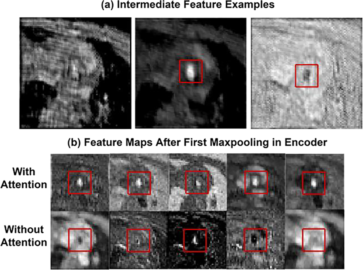
(a) shows three different examples of 80 × 80 intermediate feature maps after several layer of convolutons. (b) shows 40 × 40 feature maps after first maxpooling in encoder with (first row) and without (second row) attention block in the architecture. From observation flow region is a dominant feature in the feature maps when network is trained with attention block in the architecture. Rectangular red box in the images indicates the flow region.
The input to spatial attention is the channel attention weighted feature map –
| (3) |
Here ⊗ denotes element wise multiplication. In spatial attention block, average pooling and max pooling are both applied in the feature map. Local maxpooling in spatial attention identifies the flow region with brighter pixels locally in each feature map, thus ensuring more weight in the flow region and local average pooling understands the total extent of each feature map. The combination of maxpooling and average pooling has been empirically proven to improve the representation power of the network [25]. Pooled features are concatenated and convolved by a convolution layer and generate spatial attention As-
| (4) |
Here, X3×3 denotes a 2D convolution with kernel size 3 × 3. Output feature map after attention will be where-
| (5) |
Here, is the refined feature map after sequential channel and spatial attention aiming to improve the reconstruction performance. Fig. 3(b) shows feature maps after the first maxpooling in encoder with and without attention. The first row of fig. 3(b) shows several examples of 40 × 40 feature maps after first maxpooling in encoder when the network is trained with the proposed architecture. The second row shows several feature maps after the first maxpooling, excluding attention block in the architecture while training. From feature map observation, after the first maxpooling operation in the encoder, flow region is hardly present in the feature maps without attention block. In contrast, flow region is a dominant feature in the feature maps when network is trained with attention block in the architecture. Attention block after each residual block thus ensures efficient flow information propagation by giving importance to the flow features. Output from the final attention block in the decoder goes into a convolutional layer consisting of 2 filters, which results in 2 channel outputs of the same resolution as input.
Loss Function:
Pixel wise square error is considered as network loss function
| (6) |
Here, ur,2D represents, reconstructed 2D complex image from the network and u2D represents, labelled fully sampled 2D complex image.
C. Undersampling Technique
In the compressive sensing approach, it is necessary to have a random sampling pattern in the phase encoding direction to avoid artifacts in the reconstruction. However, in the deep learning approaches, uniform undersampling or randomization in the phase encoding direction- both were used by previous studies [14], [15] to create subsampled k-space to train the network. [30] proposed a sampling augmented training strategy by using varying sampling pattern in k-space. According to [30], instead of using a fixed undersampling pattern, a varying undersampling pattern in k-space creates different artifacts in the zero-filled reconstructed image so that the network can learn a wide range of undersampling artifacts during the training. In 4D flow MRI, 3D k-space over time is acquired. For 3D acquisition, random undersampling can be implemented in Ky –Kz plane. [39] implemented random undersampling in Ky –Kz plane, keeping the low frequency region fully sampled, and performing random undersampling in the high frequency region. [36] implemented a cartesian random undersampling in Ky–Kz–t plane, where randomization is applied not only in Ky –Kz plane but also in Ky –t plane. We similarly adopted a random Ky–Kz–t sampling pattern for the undersampling in k-space so that randomization in both planes will create variation in artifacts in the zero-filled images and help the network in better generalization. A variable density Poisson-disk probability function assigns the highest probability of sampling in the center of Ky–Kz plane. We repeat the generation process Nt number of times that creates Ky –Kz sampling patterns along Nt temporal phases. The low frequency of Ky –Kz plane are fully sampled at all time points. Fig. 4(a) shows 20% cartesian sampling pattern in Ky–Kz plane, where each dot represents a readout line in k-space and 4(b) shows 20% cartesian sampling pattern at different timepoints.
Fig. 4:
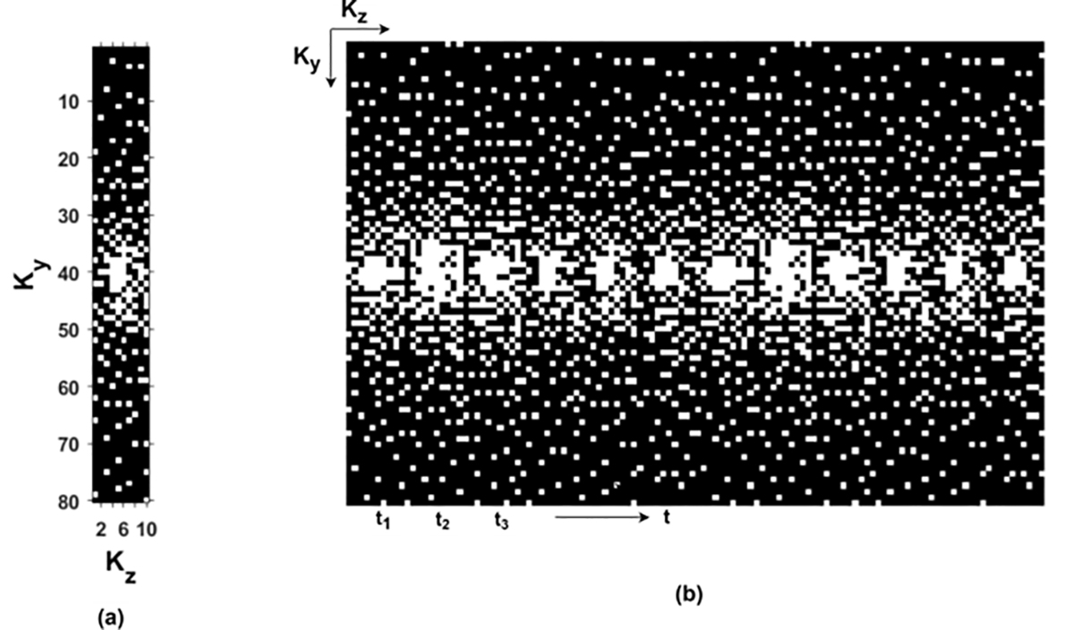
Example of random cartesian undersampling in k-space (a) 20% cartesian sampling pattern in Ky–Kz plane where each dot represents a readout line in k-space. (b) 20% cartesian sampling pattern in different timepoints.
D. Data Acquisition and Network Training
The study was approved by the institutional review board at the Veterans Affairs Medical Center in Louisville, Kentucky. Healthy volunteers, as well as patients with severe aortic stenosis (AS) were scanned, concluding 18 human subject scans. It should be noted that due to an oversight by authors, the healthy volunteers, despite having given informed consent, were not initially approved by the IRB to be scanned since they were not US Veterans. However, the IRB subsequently approved the use of their data. Among 18 subject scans, 10 of them were patient scans, and 8 were healthy volunteers. Patients were recruited from the Cardiology Clinic at the Robley Rex VA Medical Center (all male subjects, age 69 ± 8.6). Severe AS was defined based on Doppler echocardiography measurements: peak systolic velocity greater than 3.5 m/s, effective orifice area (EOA) less than 1 cm2, or transvalvular pressure gradient (TVPG) ≥ 40 mmHg. 4D flow data of blood flow through the aortic valve were collected with Cartesian readout on a 1.5T Phillips Achieva scanner with a 16 channel XL Torso coil. The acquisition employed 4D flow encoding with Cartesian read-out, which employed x, y, and z velocity encoding as part of the same acquisition. A four-point balanced Hadamard encoding [5, 43] was used in the pulse sequence during acquisition which allows for improved velocity to noise ratio in each flow encoding direction. The scan parameters for patient data were, TE= 3ms, TR= 14ms, matrix size=80×80×10, field of View=200×200×50 (mm3), resolution= 2.5×2.5×5 (mm), slice thickness= 5mm, number of slices=10, flip angle= 80, 400<venc<500 (cm/s), scan time= 15 min(approximately). Data were acquired over a variable number of heart phases, with a minimum of 16 phases. The number of phases selected was based on whether the addition of a heart phase was possible and/or added time to the scan. The navigator window length was set to 100 mm, with an acceptance window of 7 mm. The FOV for all the subjects included 1–2 slices proximal to the aortic valve, with the remaining 8–9 slices distal to the valve. For consistency in the training data, we considered 15 temporal phases for all subjects. Respiratory gating with navigators was used. Phase image values were normalized to [−π, π] range and magnitude image values in the [1, 10] range. k-space data were downsampled retrospectively with 20%, 30% and 40% sampling. From zero-filled reconstructed images, each time frame from every slice was taken as a separate training example. Despite this, the training dataset for each velocity encoding is relatively small, containing only 2700 images. Therefore, we augmented the dataset by rotating each image between [0, 2π] in 10-degree increments, creating a dataset of 94,500 images for each encoding training. We split the dataset into training and testing set via 9-fold cross validation on 18 subjects. In 8 folds, 16 subject data (including augmentations) were used for training, and the remaining data for 2 subjects, which were in the ninth fold, were used for testing. To report the performance measures, this process was repeated 9 times. A batch size of 32 was used to train the network. Network weights were initialized using normal distribution with a standard deviation of 0.01. Pixel wise mean squared error between the output and labelled image was considered as loss function. RMSprop optimizer [35] was used to minimize the loss function with a learning rate of 0.0001. After every 50-epoch learning rate was decreased by half. Maximum epoch was set as 400, and early stopping was used as momentum to avoid overfitting. We used Nvidia’s GeForce GTX 1050 Ti GPU and training took 1 day. The experiments in this study were performed using Keras with Tensorflow whose back end is Python 2.7.
E. Performance Evaluation
Usually, reconstruction of MRI modality where magnitude image is of main importance, structural similarity index measurement and NMSE are chosen as performance measure instead of F1 score and dice co-efficient that usually used in classification and segmentation. However, in the 4D Flow reconstruction problem, flow information is of central importance, and performance measures were chosen according to the flow information or velocity vector recovery by the previous state-of-the-art methods [36], [11], [16], etc. Similarly, the performance measures in this manuscript are also chosen to reflect the effectiveness of velocity vector recovery. The reconstructed image is a 2-D complex image containing magnitude and phase information in 2-D. For quantitative image evaluation, normalized mean square error (NMSE) in all encoding direction, slice and time position gives an objective comparison between the reference 4D flow u ∈ CN and reconstructed 4D flow ur ∈ CN -
| (7) |
Here, u(t, z, i) and ur(t, z, i) are reference and reconstructed 2-D complex image at time position t, slice position z and velocity encoding direction i. From reconstructed complex image in three encoding direction, phase image of FH, AP and RL and corresponding magnitude image is calculated. Phase is encoded within the range [𝜋 − 𝜋]. From phase image, velocity mapping is done by - . Here, venc is velocity encoding parameter which is set during acquisition. It is set in a way so that the maximum velocity in a flow direction corresponds to 180-degree phase shift. After computing velocity mapped image in FH, AP, and RL direction, region of interest (ROI) that contains blood flow is segmented by GTFlow (GyroTools, Zurich, Switzerland) software. GTFlow allows drawing of vessel contours with b-spline curves in different regions of the aorta and creates very accurate segmentation of the vessel after the user selects a few anchor points on the vessel boundary. Same ROI is used for velocity image in all encoding direction. Velocity mapped image in FH, AP and RL direction gives 3-D velocity vectors in the ROI. 3-D velocity vectors in the ROI from reconstructed image are compared with 3-D velocity vectors from fully sampled image. Relative velocity error and Angular error of 3-D velocity is measured in 2-D slices and averaged over all the slices and time position to measure error in 4D flow by –
| (8) |
| (9) |
Here, υref(t, z) and υr(t, z) denotes 3D velocity vectors in ROI region from reference and reconstructed images in slice position z and time position t. Along with velocity accuracy measurement, two other flow parameter- flow rate and peak velocity is considered for performance evaluation. Flow rate in a 2-D slice is calculated by average velocity in through plane direction in flow region multiplied by flow area. Accuracy of flow rate is measured by calculating root mean square error (RMSE) between flow rate from reconstructed velocity mapped image and fully sampled velocity mapped image at all time point and slice location. RMSE of peak velocity at all slice location and over all time frame is also measured for performance evaluation-
| (10) |
| (11) |
In (10), Qref(t, z), Qr(t, z) denotes flow rate from a 2-D slice in reference image and reconstructed image. Similarly, in (11) , denotes peak velocity in 2-D slice in reference image and reconstructed image. Proposed method is compared with one state of the art iterative compressed sensing regularization method [20] where total variation is used for sparsity in cardiac phase dimension of 4D flow data. Comparison is made with three other image domain learning based reconstruction approach [21], [37] and [38]. [21] adopted a U-net architecture for phase contrast MRI reconstruction in FH encoding direction with 2 channel complex input and output. [37] proposed a GAN based reconstruction approach namely DAGAN and [38] proposed an attention-based reconstruction approach namely SAT-net. DAGAN uses a U-net-based architecture as the generator and a CNN-based classification network as the discriminator. SAT-net proposes a densely connected U-net with local and global shortcuts and an attention mechanism integrated with each convolution layer. For 4D Flow reconstruction, all networks are trained and tested at three encoding directions separately for all subjects. Same 2 channel zero-filled reconstructed images are used to train the comparison networks. Adam optimizer with initial learning rate of 0.0001, β1 = 0.9, β2 = 0.999 were used for DAGAN network. Learning rate was halved every 5 epoch. For SAT-net, initial learning rate of 0.001, β1 = 0.9, β2 = 0.999 were used and after each 50 epoch learning rate was decreased by half. Batch size of 16 was used for the network training. 9 fold cross validation was performed where at each fold 16 subjects were used for training and 2 subjects were kept out for testing.
III. Results
Fig. 5 and Fig. 6 show reconstructed images for one healthy volunteer and one patient subject. Reconstructed axial slices are shown at aortic valve position at systole phase of the cardiac cycle for 30% subsampling in k-space. First row of Fig. 5 and Fig. 6 shows the magnitude image for the reference fully sampled image, zero-filled reconstructed image, reconstruction by TV regularization method, U-net method, proposed FlowRAU-net method, DAGAN method, and SATnet method. Second, third, and fourth row of Fig. 5 and Fig. 6 shows the corresponding velocity mapped images in FH, AP, and RL encoding direction. Fig. 5 and Fig. 6 demonstrates that reconstructed magnitude image and velocity image by FlowRAU-net can restore structural information and fine details of original image discarded by undersampling. Though several areas of the magnitude image suffer from blurry edges and textures, the proposed method appears to restore more structural information and fine details than the reconstructed magnitude image by other methods. Velocity images in Fig. 5 and Fig. 6 contain the hemodynamic information and are restored by the proposed method without any artifact. Though velocity image by other reconstruction methods also restores the velocity information which is absent from zero-filled reconstructed image, it suffers from some degree of blurring from the reference phase image. Fig. 7 and Fig. 8 show the magnitude of velocity in flow region in reconstructed images for one healthy volunteer and one patient subject with aortic stenosis. Velocity magnitude is calculated as ‖υ‖2 where υ = (υFH, υAP, υRL). The first row of Fig. 7 and Fig. 8 shows the flow region in a red rectangular box in an axial slice of velocity mapped image. The second row shows the velocity magnitude ‖υ‖2 in the flow region. Different columns in Fig. 7 and Fig. 8 represent velocity magnitude for reconstructed images by proposed FlowRAU-net and other comparison methods. Third row shows the velocity magnitude error as the absolute difference of velocity magnitude of reference and comparison methods. Corresponding relative velocity error is shown in Fig. 7 and Fig. 8 where FlowRAU-net method shows minimum relative velocity error than the other methods. Important decisions of diagnosis and prognosis is taken by the clinicians by visualizing the complex flow pattern of the 4D Flow pathline. That is why it is important to check if the reconstructed 4D flow by the proposed method has good agreement with the ground truth fully sampled 4D flow MRI in 3D visualization of hemodynamic pathline. Fig. 9 shows 3D path-line visualization using GTFlow Software of reference fully sampled 4D flow and reconstructed 4D flow by FlowRAU-net for 30% k-space undersampling of a healthy volunteer. Corresponding velocity magnitude in an axial slice of aortic valve is shown at the right corner of each image. Pathline of reference 4D flow and reconstructed 4D Flow by proposed method shows excellent agreement. Volumetric flow and peak velocity over time are important hemodynamic parameters with great clinical value. Fig. 10(a) shows blood flow profile comparison at aortic valve position for one healthy subject in the first column and patient subject in the second column for different reconstruction methods at 30% k-space subsampling. Fig. 10(b) shows peak velocity profile comparison for a healthy subject in the first column and patient subject in the second column. From Fig. 10(a) and (b), proposed method follows the flow profile and peak velocity profile better than the other four methods. From Fig. 10(a) and Fig. 10(b), the reconstructed flow rate and peak velocity profile by the proposed method almost align with the reference whereas, the other reconstructed methods show a larger deviation from the reference. For quantitative measurement of reconstruction error- Image NMSE, Relative Velocity Error, Angular Error, Flow Error, and Peak Velocity Error is calculated according to eqn. (7) – eqn. (11). The average measurement for all subjects with standard deviation is shown in Table I for three different subsampling of k-space. From Table I, the proposed FlowRAU-net outperforms other methods in image NMSE measurement in all three k-space sampling factors. Relative velocity error and angular error are measured to compare the accuracy of velocity vectors among different methods. Though TV regularization and three other deep learning methods have comparative errors, especially when subsampling is the lowest (20%), the proposed FlowRAU-net shows minimum error in both angular error and relative velocity error in all three subsampling factors. This is also evident from Fig. 7 and Fig. 8, which show FlowRAU-net follows reference velocity magnitude more accurately than the other methods. Average flow error and average peak velocity error are calculated according to eqn. (10) and (11), and results are shown for three k-space subsampling factors. At 20% subsampling factor all comparative methods show quite large flow error and velocity error. However, error minimizes at 30%, and 40% k-space subsampling and FlowRAU-net shows lower errors than the other methods.
Fig. 5:
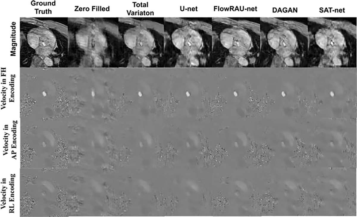
Comparison of 4D Flow reconstructed images for various techniques in one healthy in-vivo subject. The first row shows magnitude image (in one encoding direction). The second, third, and fourth row shows velocity mapped image at FH, AP and RL direction from the reference image, the zero- filled reconstructed image, and the image reconstructed by U-net, TV regularization, DAGAN, SAT-net and proposed FlowRAU-net method. The images are in the peak systole phase of the cardiac cycle and is exactly at the location of the aortic valve.
Fig. 6:
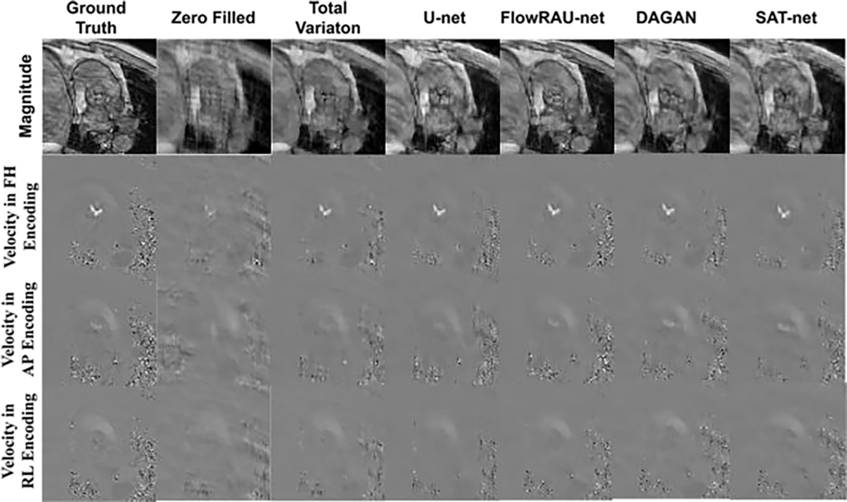
Comparison of 4D Flow reconstructed images for various techniques in one patient in-vivo. The first row shows magnitude image (in one encoding direction). The second, third, and fourth row shows velocity mapped image at FH, AP and RL direction from the reference image, the zero- filled reconstructed image, and the image reconstructed by U-net, TV regularization, DAGAN, SAT-net and proposed FlowRAU-net method. The images are in the peak systole phase of the cardiac cycle and is exactly at the location of the aortic valve.
Fig. 7:
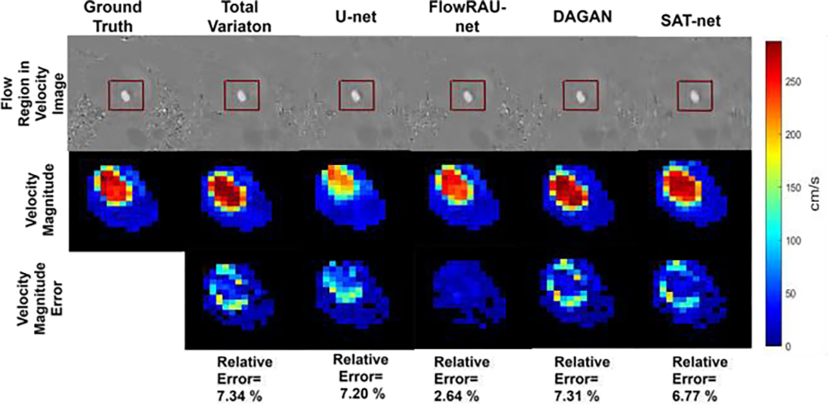
Comparison of velocity magnitude in flow region for different reconstruction methods in one healthy subject. The first row shows the blood flow region in a velocity image (FH Encoding) by a rectangular red box. The second row shows the zoomed-in velocity magnitude, and the third row shows the velocity magnitude error image as the absolute difference from the reference image. Velocity magnitude images are shown at an axial slice of aortic valve location and at peak systole phase of the cardiac cycle.
Fig. 8:
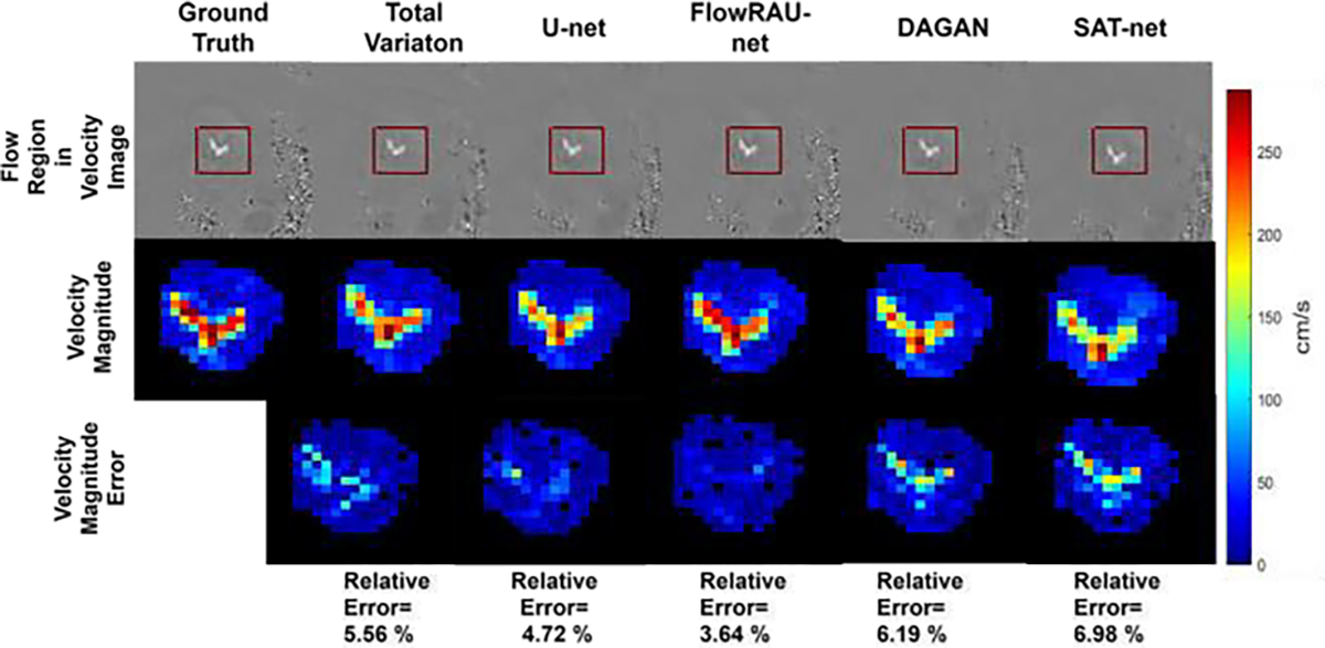
Comparison of velocity magnitude in flow region for different reconstruction methods in one patient in-vivo. The first row shows the blood flow region in a velocity image (FH Encoding) by a rectangular red box. The second row shows the zoomed-in velocity magnitude, and the third row shows the velocity magnitude error image as the absolute difference from the reference image. Velocity magnitude images are shown at an axial slice of aortic valve location and at peak systole phase of the cardiac cycle.
Fig. 9:
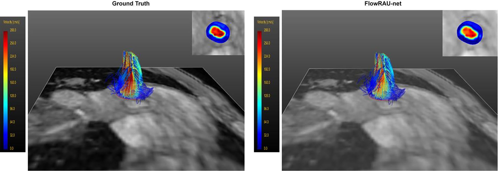
Velocity pathline in 3D view for flow at the level of aortic valve at peak systole in a healthy volunteer. The pathline of reference fully sampled 4D flow is shown on the left and the pathline for reconstructed 4D flow by FlowRAU-net is shown on the right. Corresponding velocity magnitude in an axial slice of the aortic valve is shown in the inset.
Fig. 10:
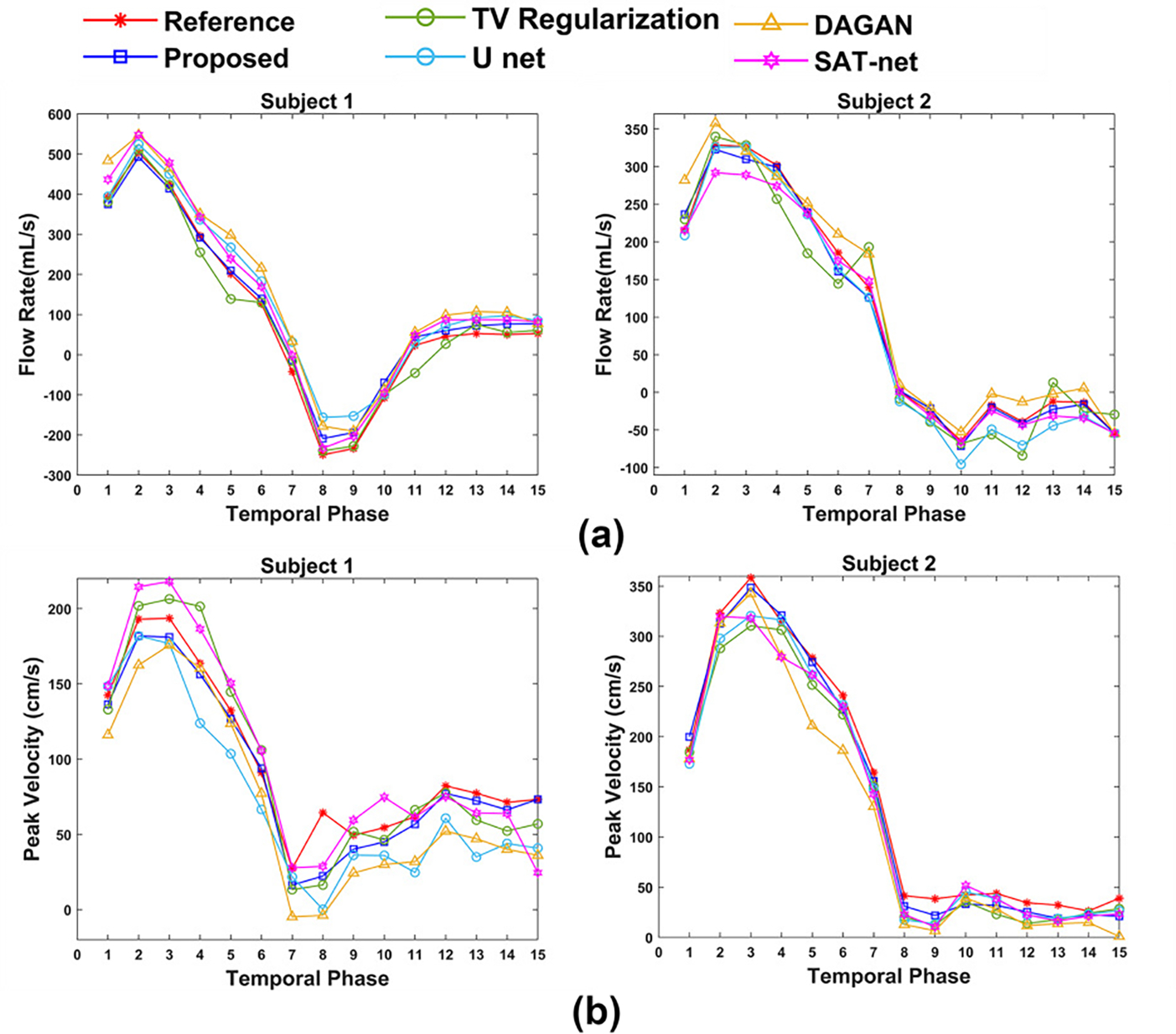
(a) shows flow rate with time and (b) shows peak velocity with time from reference velocity image and reconstructed image for 30% k-space subsampling by TV Regularization method, U-net method, DAGAN method, SAT-net method and proposed FlowRAU-net method in two subjects (subject 1= healthy volunteer, subject 2= patient with Aortic Stenosis), calculated close to the level of the aortic valve.
TABLE I.
Average Quantitative Measurement of All Subjects Comparing Proposed FlowRAU-net Method and Four State of the Art Reconstruction Methods
| Parameter | k-space Sampling(%) | Dynamic TV [20] | U-net [14,21] | DAGAN[37] | SAT-net[38] | FlowRAU-net |
|---|---|---|---|---|---|---|
|
| ||||||
| Image NMSE (%) | 20% | 6.133 ± 0.33 | 6.552 ± 0.31 | 7.231 ± 0.41 | 6.310 ± 0.39 | 5.198 ± 0.28 |
| 30% | 5.931± 0.20 | 4.232 ± 0.22 | 5.566 ± 0.11 | 5.803 ± 0.10 | 3.225 ± 0.17 | |
| 40% | 4.015 ± 0.14 | 3.955 ± 0.20 | 3.872 ± 0.12 | 4.908 ± 0.17 | 2.194 ± 0.12 | |
|
| ||||||
| Relative Velocity Error(%) | 20% | 15.108 ± 2.28 | 18.382 ± 3.51 | 19.455 ± 3.94 | 21.788 ± 4.16 | 15.137 ± 2.53 |
| 30% | 14.312 ± 2.75 | 14.363 ± 2.77 | 14.271± 3.76 | 15.567 ± 3.83 | 11.077 ± 2.44 | |
| 40% | 11.011 ± 2.12 | 12.221 ± 2.85 | 13.898± 2.32 | 12.927 ± 2.68 | 10.329 ± 2.18 | |
|
| ||||||
| Angular Error (degree) | 20% | 18.112± 3.93 | 17.922± 3.98 | 18.297± 3.99 | 16.979± 3.92 | 17.164 ± 3.10 |
| 30% | 17.433± 3.931 | 16.856± 2.91 | 16.864± 2.04 | 14.314± 2.99 | 14.394± 3.29 | |
| 40% | 13.101± 2.23 | 13.994± 3.11 | 14.221± 3.23 | 13.017± 3.53 | 12.575± 3.98 | |
|
| ||||||
| Flow Error (mL/s) | 20% | 48.572± 7.37 | 52.113± 9.33 | 50.491± 7.17 | 55.960± 7.30 | 45.434± 8.39 |
| 30% | 31.164± 5.54 | 30.5297± 6.10 | 32.633± 5.41 | 37.809± 5.33 | 27.748± 6.05 | |
| 40% | 22.253± 4.32 | 23.643± 6.11 | 23.989± 4.62 | 28.236± 4.49 | 18.196± 4.12 | |
|
| ||||||
| Peak Velocity Error (cm/s) | 20% | 37.018± 6.45 | 37.353± 7.87 | 36.880± 7.97 | 38.154± 9.15 | 36.400± 6.25 |
| 30% | 22.9810± 6.34 | 20.226± 7.61 | 17.170± 6.57 | 22.476± 8.59 | 15.9445± 5.30 | |
| 40% | 17.092± 6.11 | 13.337± 6.85 | 12.814± 6.65 | 15.915± 7.32 | 10.322± 5.13 | |
IV. Discussion
In this paper, an image domain learning-based 4D flow reconstruction is suggested by reducing artifacts from zero-filled reconstructed complex image. Varying sampling pattern with cardiac phase in k-space is used for variation in artifact in zero-filled reconstructed complex images and robust learning of proposed network. Adopting residual block and attention block in U-net architecture significantly improves qualitative and quantitative measurement of image, 3-D velocity vectors, and flow parameters. Using local residual connection in the residual block enables efficient weight updating during the backpropagation, and channel, and spatial attention helps emphasize important flow information in the flow image. From Fig. 3(b), when no attention block is used in the architecture, the network fails to recognize the flow region as an important feature in the feature maps (low prominence). That is why our proposed architecture performs better than a basic U-net architecture. DAGAN employs a U-net as a generator network and a CNN-based classification network as a discriminator and does not emphasize the flow features in the image. In the SAT-net, a self-attention is proposed where weight in each pixel is calculated by a 1×1 convolution and a linear and embedded gaussian function. No inter-channel dependency is observed, which would help to locate the flow feature in the image. No local and global pooling is performed, which would be important to give importance to the flow region as brighter pixels with high prominence. The combination of residual block and channel and spatial attention block in the encoder-decoder network helps efficient propagation of flow information during the learning process and provides excellent reconstruction performance. From Table I, it is evident that the proposed FlowRAU-net outperforms state of the art compressed sensing method and deep learning-based reconstruction methods in all the measurements for different sampling factors. When undersampling in k-space is 20%, performance goes down in all the reconstruction techniques, notably resulting in large errors in flow parameters and velocity measurements. Fig. 11 shows reconstructed velocity image in FH direction for 20%, 30%, and 40% sampling in k-space and corresponding velocity magnitude and relative error. From Figure 11, when k-space subsampling goes up at 40%, reconstructed velocity magnitude is almost close to reference fully sampled velocity magnitude with minimal error. Reconstruction time is significantly low in the proposed method compared to compressed sensing TV regularization method. 4D flow reconstruction by compressed sensing TV regularization takes approximately 8 minutes, whereas a single 2D complex image takes 150ms to reconstruct by FlowRAU-net and total 4D flow data for one subject requires 69 seconds. Training and reconstruction time in FlowRAU-net and U-net is almost similar but adopting residual block and attention block in FlowRAU-net better adopts with the data and yields lower training and validation error during training via 9-fold cross validation. Training and validation loss curve of U-net and FlowRAU-net for a single fold training in FH direction is shown in Fig. 12(a). Fig. 12(b) shows training and validation loss at convergence during each fold training of 9- fold cross validation. Proposed FlowRAU-net results in lower validation mean square error (MSE) loss during training at every fold. Proposed FlowRAU-net architecture has 3 residual attention (RA) blocks in encoder and 3 maxpooling function. Network performance is investigated by increasing RA block and maxpooling in the encoder and upsampling in the decoder. However, increasing RA block results increase in the network parameter. Though the training loss decreases with increased complexity in the network, validation loss increases and overfits. Different number of convolution block in residual block is also investigated in the architecture. Increasing the convolution block number from 3 to 4 in the residual block does not improve the accuracy in the training. However, increasing the convolution block number from 3 to 5 and higher number leads to overfitting in the training.
Fig. 11:
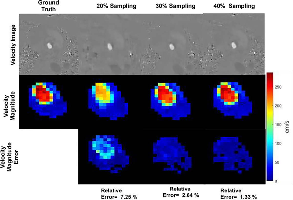
Reconstruction result for 20%, 30%, and 40% k-space sampling in a healthy volunteer for proposed FlowRAU-net. The First row shows reconstructed velocity image in the FH direction. Second and third row show corresponding zoomed-in velocity magnitude and velocity magnitude error. Images are shown at an axial slice of aortic valve location and at peak systole phase of the cardiac cycle.
Fig. 12:
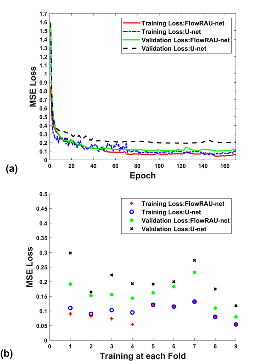
(a) Training and validation loss curve of U-net and FlowRAU-net for a single fold training in FH direction (b) Training and validation loss at the convergence of U-net and FlowRAU-net at each fold during the training of 9-fold cross-validation.
A. Ablation Studies
We proposed a U-net based architecture where the integrated residual block and attention block works as the backbone of the U-net. In the attention block, channel attention and spatial attention are applied consecutively. To evaluate the impact of the residual block and attention block in network architecture, we have performed reconstruction and measured reconstruction results for several variations in the architecture. In the first case, reconstruction is done with only residual block as the backbone of U-net, eliminating attention block from the architecture (Case-I). For implementation, the same residual block as Fig. 2(b) is used consists of convolution layer, batch normalization, and ReLU activation function. The number of convolution blocks in residual block and the number of filters in encoder and decoder is same as the architecture in the proposed network. In the second case study, only spatial attention (SA) is added with Resnet block eliminating channel attention (CA) from the architecture (Case-II). In the third case study, only channel attention (CA) only spatial attention (SA) is added with Resnet block eliminating channel attention (CA) from the architecture (Case-II). In the third case study, only channel attention (CA) is added with residual attention block eliminating spatial attention (SA) from the architecture (Case-III). The fourth case study is the proposed architecture where both channel and spatial attention is used (Case-IV). Pixel wise mean squared error is considered as loss function, and RMSprop optimizer with a learning rate of 0.0001 is used in all the cases. Reconstruction for the different case study is performed for 30% k-space sampling. Reconstruction results for different case studies are compared in terms of image quality, velocity vector accuracy, and flow parameters. Eqn. (7)– Eqn (11) is used for evaluation and averaged over all the subjects of 4D flow. Table II shows reconstruction results for the case study in network architecture. Table II shows that when Resnet block (Case I) is used instead of convolutional blocks in U-net, average NMSE, Rel. Velocity Error and Angular Error are reduced by several percentages from U-net. However, in Case II, when spatial attention is used with Resnet block, we see a slight improvement in the network for all the error measures in all the measurements. But when Channel attention is used along with spatial attention, it shows much improvement in the reconstruction results. Fig. 13 shows the magnitude of velocity in flow region in reconstructed images from different case studies in the aortic valve region of one healthy subject. From Fig. 13, it is evident that residual block along with CA and SA block provides more accuracy than other network architectures.
TABLE II.
Average Quantitative Measurement of All Subjects for Ablation Studies in Network Architecture.
| Parameter | Resnet Block (Case I) | Resnet Block+SA (Case II) | Resnet Block+CA (Case III) | Resnet Block+SACA (Case IV) |
|---|---|---|---|---|
| NMSE (%) | 4.011%± 0.314% | 3.962%± 0.425% | 3.477%± 0.203% | 3.225% ± 0.179% |
| Rel. Velocity Error (%) | 13.165%± 2.672% | 12.977%± 2.785% | 11.230% ± 2.211% | 11.077% ± 2.441% |
| Angular Error(degree) | 16.6660± 4.170 | 16.1350± 4.061 | 15.733± 3.750 | 14.394± 3.293 |
| Flow Error (mL/s) | 29.3075± 6.321 | 29.2311± 6.410 | 27.9810± 6.285 | 27.748± 6.052 |
| Peak Velocity Error (cm/s) | 18.3902± 7.643 | 17.2663± 6.411 | 17.0321± 5.211 | 15.9445± 5.308 |
Fig. 13:
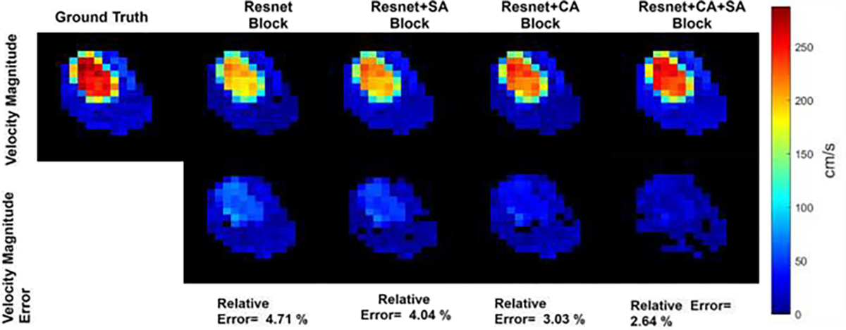
3D velocity vector magnitude of reference ground truth and reconstructed image for different case studies in network architecture. Resnet block, along with CA and SA block as the backbone of U-net, provides the highest accuracy in reconstruction. Velocity magnitude is shown at the region of interest of aortic valve location and at peak systole phase of the cardiac cycle for one subject.
B. Limitation of the Study
Though the proposed FlowRAU-net produces a fast and accurate reconstruction of 4D flow MRI, there are some limitations to the study. First, the proposed network is a 2D reconstruction network that considers each time point and slice location image as a separate training sample. The reconstruction is done by learning 2D spatial features. Reconstruction by learning spatio-temporal features might result in better reconstruction accuracy. Also, reconstruction by 3D spatial feature learning might exploit 3D structural information in the data. To exploit 3D spatial feature or spatio-temporal feature, reconstruction by a 3D network is needed. However, to accomplish this, there is need to have a significantly higher number of training samples. Even with augmentation, the training size for a 3D network would remain small. Future work will involve collecting more 4D flow data for training of 3D networks and also improved training of 2D network by incorporating more training data.
V. Conclusion
This paper presents an end-to-end deep learning framework for accelerated reconstruction of 4D flow. Our proposed FlowRAU-net can learn to recover both magnitude and velocity information in all velocity encoding directions with high fidelity. Reconstruction time for the proposed method is significantly lower (69 seconds for total 4D flow data reconstruction) compared to iterative compressive sensing approaches (which result in reconstruction times on the order of 7–8 min). Although the proposed method has been applied to 4D flow MRI of aortic valvular flows, it should be applicable to other arterial flows given sufficient number of training samples. The proposed end-to-end training with an attention network provides a promising direction for accelerated 4D flow MRI with significant clinical impact.
Acknowledgments
This work was supported in part by the National Institutes of Health award 1R21-HL132263.
Contributor Information
Ruponti Nath, Medical Imaging Laboratory, Department of Electrical and Computer Engineering, University of Louisville, Louisville, KY 40292 USA.
Sean Callahan, Medical Imaging Laboratory, Department of Electrical and Computer Engineering, University of Louisville, Louisville, KY 40292 USA.
Marcus Stoddard, Department of Medicine, University of Louisville, Louisville, KY 40292 USA.
Amir A. Amini, Medical Imaging Laboratory, Department of Electrical and Computer Engineering, University of Louisville, Louisville, KY 40292 USA.
References
- [1].Kim D, Dyvorne H, Otazo R, Feng L, Sodickson D and Lee V, “Accelerated phase-contrast cine MRI using k-t SPARSE-SENSE”, Magnetic Resonance in Medicine, vol. 67, no. 4, pp. 1054–1064, 2011. [DOI] [PMC free article] [PubMed] [Google Scholar]
- [2].Carlsson M et al. , “Quantification and visualization of cardiovascular 4D velocity mapping accelerated with parallel imaging or k-t BLAST: head to head comparison and validation at 1.5 T and 3 T”, Journal of Cardiovascular Magnetic Resonance, vol. 13, no. 1, 2011. [DOI] [PMC free article] [PubMed] [Google Scholar]
- [3].Stankovic Z et al. , “K-t GRAPPA-accelerated 4D flow MRI of liver hemodynamics: influence of different acceleration factors on qualitative and quantitative assessment of blood flow”, Magnetic Resonance Materials in Physics, Biology and Medicine, vol. 28, no. 2, pp. 149–159, 2014. [DOI] [PubMed] [Google Scholar]
- [4].Kadbi M et al. , “4D UTE flow: A phase-contrast MRI technique for assessment and visualization of stenotic flows”, Magnetic Resonance in Medicine, vol. 73, no. 3, pp. 939–950, 2014. [DOI] [PubMed] [Google Scholar]
- [5].Negahdar M, Kadbi M, Kendrick M, Stoddard M and Amini A, “4 D spiral imaging of flows in stenotic phantoms and subjects with aortic stenosis”, Magnetic Resonance in Medicine, vol. 75, no. 3, pp. 1018–1029, 2016. [DOI] [PMC free article] [PubMed] [Google Scholar]
- [6].Liang D, DiBella E, Chen R and Ying L, “k-t ISD: Dynamic cardiac MR imaging using compressed sensing with iterative support detection”, Magnetic Resonance in Medicine, vol. 68, no. 1, pp. 41–53, 2011. [DOI] [PMC free article] [PubMed] [Google Scholar]
- [7].Chen Z et al. , “Accelerated 3D Coronary Vessel Wall MR Imaging Based on Compressed Sensing with a Block-Weighted Total Variation Regularization”, Applied Magnetic Resonance, vol. 48, no. 4, pp. 361–378, 2017. [Google Scholar]
- [8].Schnell S et al. , “k-t GRAPPA accelerated four-dimensional flow MRI in the aorta: Effect on scan time, image quality, and quantification of flow and wall shear stress”, Magnetic Resonance in Medicine, vol. 72, no. 2, pp. 522–533, 2013. [DOI] [PMC free article] [PubMed] [Google Scholar]
- [9].Zhao Feng, Noll D, Nielsen J and Fessler J, “Separate Magnitude and Phase Regularization via Compressed Sensing”, IEEE Transactions on Medical Imaging, vol. 31, no. 9, pp. 1713–1723, 2012. [DOI] [PMC free article] [PubMed] [Google Scholar]
- [10].Kwak Y et al. , “Accelerated aortic flow assessment with compressed sensing with and without use of the sparsity of the complex difference image”, Magnetic Resonance in Medicine, vol. 70, no. 3, pp. 851–858, 2012. [DOI] [PMC free article] [PubMed] [Google Scholar]
- [11].Rich A, Potter L, Jin N, Liu Y, Simonetti O and Ahmad R, “A Bayesian approach for 4D flow imaging of aortic valve in a single breath‐hold”, Magnetic Resonance in Medicine, vol. 81, no. 2, pp. 811–824, 2018. [DOI] [PMC free article] [PubMed] [Google Scholar]
- [12].Schlemper J, Caballero J, Hajnal J, Price A and Rueckert D, “A Deep Cascade of Convolutional Neural Networks for Dynamic MR Image Reconstruction”, IEEE Transactions on Medical Imaging, vol. 37, no. 2, pp. 491–503, 2018. [DOI] [PubMed] [Google Scholar]
- [13].Sun L, Fan Z, Ding X, Huang Y and Paisley J, “Region-of-interest undersampled MRI reconstruction: A deep convolutional neural network approach”, Magnetic Resonance Imaging, vol. 63, pp. 185–192, 2019. [DOI] [PubMed] [Google Scholar]
- [14].Hyun C, Kim H, Lee S, Lee S and Seo J, “Deep learning for undersampled MRI reconstruction”, Physics in Medicine & Biology, vol. 63, no. 13, p. 135007, 2018. [DOI] [PubMed] [Google Scholar]
- [15].Han Y, Sunwoo L and Ye J, “${k}$ -Space Deep Learning for Accelerated MRI”, IEEE Transactions on Medical Imaging, vol. 39, no. 2, pp. 377–386, 2020. [DOI] [PubMed] [Google Scholar]
- [16].Vishnevskiy V, Walheim J and Kozerke S, “Deep variational network for rapid 4D flow MRI reconstruction”, Nature Machine Intelligence, vol. 2, no. 4, pp. 228–235, 2020. [Google Scholar]
- [17].Hammernik K et al. , “Learning a variational network for reconstruction of accelerated MRI data”, Magnetic Resonance in Medicine, vol. 79, no. 6, pp. 3055–3071, 2017. [DOI] [PMC free article] [PubMed] [Google Scholar]
- [18].Maier A et al. , “Learning with known operators reduces maximum error bounds”, Nature Machine Intelligence, vol. 1, no. 8, pp. 373–380, 2019. [DOI] [PMC free article] [PubMed] [Google Scholar]
- [19].Mardani M et al. , “Deep Generative Adversarial Neural Networks for Compressive Sensing MRI”, IEEE Transactions on Medical Imaging, vol. 38, no. 1, pp. 167–179, 2019. [DOI] [PMC free article] [PubMed] [Google Scholar]
- [20].Montesinos P, Abascal J, Cussó L, Vaquero J and Desco M, “Application of the compressed sensing technique to self-gated cardiac cine sequences in small animals”, Magnetic Resonance in Medicine, vol. 72, no. 2, pp. 369–380, 2013. [DOI] [PubMed] [Google Scholar]
- [21].Nath R, Callahan S, Singam N, Stoddard M and Amini AA, “Accelerated Phase Contrast Magnetic Resonance Imaging via Deep Learning,” 2020 IEEE 17th International Symposium on Biomedical Imaging (ISBI), Iowa City, IA, USA, 2020, pp. 834–838. [Google Scholar]
- [22].Li S, Dong M, Du G and Mu X, “Attention Dense-U-Net for Automatic Breast Mass Segmentation in Digital Mammogram”, IEEE Access, vol. 7, pp. 59037–59047, 2019. [Google Scholar]
- [23].Li X, Chen H, Qi X, Dou Q, Fu C and Heng P, “H-DenseUNet: Hybrid Densely Connected UNet for Liver and Tumor Segmentation From CT Volumes”, IEEE Transactions on Medical Imaging, vol. 37, no. 12, pp. 2663–2674, 2018. [DOI] [PubMed] [Google Scholar]
- [24].Sun L, Shao W, Zhang D and Liu M, “Anatomical Attention Guided Deep Networks for ROI Segmentation of Brain MR Images”, IEEE Transactions on Medical Imaging, vol. 39, no. 6, pp. 2000–2012, 2020. [DOI] [PubMed] [Google Scholar]
- [25].Woo S, Park J, Lee J and Kweon I, “CBAM: Convolutional Block Attention Module”, in European Conference on Computer Vision, Munich, Germany, 2018, pp. 3–19. [Google Scholar]
- [26].Schlemper J et al. , “Attention gated networks: Learning to leverage salient regions in medical images”, Medical Image Analysis, vol. 53, pp. 197–207, 2019. [DOI] [PMC free article] [PubMed] [Google Scholar]
- [27].Li J, Pan Z, Liu Q and Wang Z, “Stacked U-shape Network with Channel-wise Attention for Salient Object Detection”, IEEE Transactions on Multimedia, pp. 1–1, 2020. [Google Scholar]
- [28].Kearney V, Chan J, Wang T, Perry A, Yom S and Solberg T, “Attention-enabled 3D boosted convolutional neural networks for semantic CT segmentation using deep supervision”, Physics in Medicine & Biology, vol. 64, no. 13, p. 135001, 2019. [DOI] [PubMed] [Google Scholar]
- [29].Akçakaya M, Moeller S, Weingärtner S and Uğurbil K, “Scan-specific robust artificial-neural-networks for k-space interpolation (RAKI) reconstruction: Database-free deep learning for fast imaging”, Magnetic Resonance in Medicine, vol. 81, no. 1, pp. 439–453, 2018. [DOI] [PMC free article] [PubMed] [Google Scholar]
- [30].Liu F, Samsonov A, Chen L, Kijowski R and Feng L, “SANTIS: Sampling‐Augmented Neural neTwork with Incoherent Structure for MR image reconstruction”, Magnetic Resonance in Medicine, vol. 82, no. 5, pp. 1890–1904, 2019. [DOI] [PMC free article] [PubMed] [Google Scholar]
- [31].Kofler A, Dewey M, Schaeffter T, Wald C and Kolbitsch C, “Spatio-Temporal Deep Learning-Based Undersampling Artefact Reduction for 2D Radial Cine MRI With Limited Training Data”, IEEE Transactions on Medical Imaging, vol. 39, no. 3, pp. 703–717, 2020. [DOI] [PubMed] [Google Scholar]
- [32].Griswold M et al. , “Generalized autocalibrating partially parallel acquisitions (GRAPPA)”, Magnetic Resonance in Medicine, vol. 47, no. 6, pp. 1202–1210, 2002. [DOI] [PubMed] [Google Scholar]
- [33].Pruessmann K, Weiger M, Scheidegger M and Boesiger P, “SENSE: Sensitivity encoding for fast MRI”, Magnetic Resonance in Medicine, vol. 42, no. 5, pp. 952–962, 1999. [PubMed] [Google Scholar]
- [34].Lustig M, Donoho D and Pauly J, “Sparse MRI: The application of compressed sensing for rapid MR imaging”, Magnetic Resonance in Medicine, vol. 58, no. 6, pp. 1182–1195, 2007. [DOI] [PubMed] [Google Scholar]
- [35].“RMSprop - Optimization algorithms | Coursera”, Coursera, 2021. [Online]. Available: https://www.coursera.org/lecture/deep-neural-network/rmsprop-BhJlm.
- [36].Liu J, Dyverfeldt P, Acevedo-Bolton G, Hope M and Saloner D, “Highly accelerated aortic 4D flow MR imaging with variable-density random undersampling”, Magnetic Resonance Imaging, vol. 32, no. 8, pp. 1012–1020, 2014. Available: 10.1016/j.mri.2014.05.004. [DOI] [PMC free article] [PubMed] [Google Scholar]
- [37].Yang G et al. , “DAGAN: Deep De-Aliasing Generative Adversarial Networks for Fast Compressed Sensing MRI Reconstruction”, IEEE Transactions on Medical Imaging, vol. 37, no. 6, pp. 1310–1321, 2018. Available: 10.1109/tmi.2017.2785879. [DOI] [PubMed] [Google Scholar]
- [38].Wu Y, Ma Y, Liu J, Du J and Xing L, “Self-attention convolutional neural network for improved MR image reconstruction”, Information Sciences, vol. 490, pp. 317–328, 2019. Available: 10.1016/j.ins.2019.03.080. [DOI] [PMC free article] [PubMed] [Google Scholar]
- [39].Basha T, Akçakaya M, Goddu B, Berg S and Nezafat R, “Accelerated three-dimensional cine phase contrast imaging using randomly undersampled echo planar imaging with compressed sensing reconstruction”, NMR in Biomedicine, p. n/a–n/a, 2014. Available: 10.1002/nbm.3225 [DOI] [PubMed] [Google Scholar]
- [40].Neuhaus E, Weiss K, Bastkowski R, Koopmann J, Maintz D and Giese D, “Accelerated aortic 4D flow cardiovascular magnetic resonance using compressed sensing: applicability, validation and clinical integration”, Journal of Cardiovascular Magnetic Resonance, vol. 21, no. 1, 2019. Available: 10.1186/s12968-019-0573-0. [DOI] [PMC free article] [PubMed] [Google Scholar]
- [41].Huang Q, Yang D, Wu P, Qu H, Yi J and Metaxas D, “MRI Reconstruction via Cascaded Channel-Wise Attention Network,” 2020 IEEE 17th International Symposium on Biomedical Imaging (ISBI), Iowa City, IA, USA, 2020, pp. 834–838. [Google Scholar]
- [42].Haji‐Valizadeh H et al. , “Highly accelerated free‐breathing real‐time phase contrast cardiovascular MRI via complex‐difference deep learning”, Magnetic Resonance in Medicine, vol. 86, no. 2, pp. 804–819, 2021. Available: 10.1002/mrm.28750. [DOI] [PMC free article] [PubMed] [Google Scholar]
- [43].Dumoulin C, Souza S, Darrow R, Pelc N, Adams W and Ash S, “Simultaneous acquisition of phase-contrast angiograms and stationary-tissue images with Hadamard encoding of flow-induced phase shifts”, Journal of Magnetic Resonance Imaging, vol. 1, no. 4, pp. 399–404, 1991. Available: 10.1002/jmri.1880010 [DOI] [PubMed] [Google Scholar]


