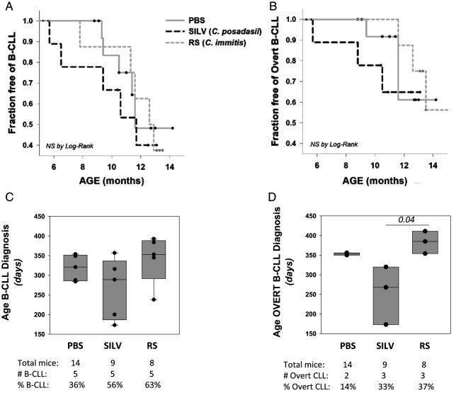
FIGURE 4.

Statistical analysis of B-CLL incidence with age.

(A) Kaplan–Meier incidence curves, representing the percentage of each cohort that is B-CLL–free over time. Small filled circles stand for censored events, reflecting mouse death without a B-CLL diagnosis. (B) Kaplan–Meier incidence curve, representing the percentage of each cohort that is free of overt B-CLL over time. PBS cohort, solid gray; SILV, dashed black; RS, short dash gray. Differences observed in (A) or (B) plots did not reach statistical significance by log-rank analysis. (C) Boxplot analysis of pooled data representing age at B-CLL diagnosis within each cohort. Boxes show median levels, with upper and lower quartiles and whiskers representing variability outside the quartiles. Overlaid black circles represent values of individual mice. Statistical analysis (Kruskal–Wallis one-way ANOVA on ranks) showed no significant difference between these groups (p = 0.491). (D) Boxplot of pooled data representing age at overt B-CLL diagnosis within each cohort. Statistical analysis (as above) revealed a statistically significant difference between these groups (p = 0.025). B-CLL cases in the PBS cohort were insufficient to make pairwise comparisons with other cohorts through the unpaired, two-sided t test. Nonetheless, ages for overt B-CLL diagnosis in the SILV cohort were statistically different from those in the RS cohort (p = 0.03) by the latter analysis.