Characterizing variations in ambient PM_2.5 concentrations at the U.S. Embassy in Dhaka, Bangladesh using observations and the CMAQ modeling system

Abstract

We analyze hourly PM_2.5 (particles with an aerodynamic diameter of ≤ 2.5 μm) concentrations measured at the U.S. Embassy in Dhaka over the 2016 – 2021 time period and find that concentrations are seasonally dependent with the highest occurring in winter and the lowest in monsoon seasons. Mean winter PM_2.5 concentrations reached ~165–175 μg/m³ while monsoon concentrations remained ~30–35 μg/m³. Annual mean PM_2.5 concentration reached ~5–6 times greater than the Bangladesh annual PM_2.5 standard of 15 μg/m³. The number of days exceeding the daily PM_2.5 standard of 65 μg/m³ in a year approached nearly 50%. Daily-mean PM_2.5 concentrations remained elevated (>65 μg/m³) for more than 80 consecutive days. Night-time concentrations were greater than daytime concentrations. The comparison of results obtained from the Community Multiscale Air Quality (CMAQ) model simulations over the Northern Hemisphere using 108-km horizontal grids with observed data suggests that the model can reproduce the seasonal variation of observed data but underpredicts observed PM_2.5 in winter months with a normalized mean bias of 13–32%. In the model, organic aerosol is the largest component of PM_2.5, of which secondary organic aerosol plays a dominant role. Transboundary pollution has a large impact on the PM_2.5 concentration in Dhaka, with an annual mean contribution of ~40 μg/m³.

1.0. Introduction

Bangladesh has tropical weather with persistent high temperature and humidity over most of the year. It has four climatological seasons: winter (December-February), pre-monsoon (March-May), monsoon (June-September) and post-monsoon (October-November) (Shahid, 2012). Winter is characterized with little to no rainfall while monsoon has heavy rainfall (Azad and Kitada, 1998; Shahid, 2012; Khan et al., 2019). The seasonal mean minimum temperatures in Dhaka range between 13–26°C, while the seasonal mean maximum temperatures range between 27–34°C (Azad and Kitada, 1998). The lowest wind speed occurs in post-monsoon and winter seasons with higher wind speed occuring in pre-monsoon and monsoon seasons. Dhaka is the capital of Bangladesh and home to more than 21 million people (https://worldpopulationreview.com, accessed on 8/13/2022). The economy of Bangladesh has been growing rapidly. Dhaka is the center of economic activity in Bangladesh and rising emissions associated with demands of rapid urban growth has led to severe air pollution. Air quality in Dhaka is affected by numerous sources: motor vehicles, two-stroke engines, brick kilns, re-suspended road dust, soil dust, metal smelters, industrial activities, shipping and aviation activities, residential combustion, agricultural residue burning, refuse burning, construction activities, sea-salt, and transboundary pollution (Azad and Kitada, 1998; Begum et al., 2010; Iqbal, 2011; Rana et al., 2016b; Begum and Hopke, 2019; Salam et al., 2021). About 1,000 brick kilns are operated near Dhaka and the neighboring districts that release emissions affecting air quality in Dhaka (Begum and Hopke, 2018). Poorly maintained vehicles and excessive traffic congestions also contribute to air pollution in Dhaka (Rahman, et al., 2019). Several studies have reported the contributions of different sources to atmospheric aerosols in Bangladesh (Begum et al., 2004; Begum et al., 2005; Begum et al., 2010; Begum et al., 2018; Begum et al., 2019). Begum and co-workers (Begum et al., 2004 and Begum et al., 2005) collected fine and coarse particles using a ‘Gent’ stacked filter sampler (Hopke et al., 1997) in Dhaka in 2001–2002, analyzed the samples using proton induced X-ray emission technique, and further analyzed the resulting data for source identification using the Positive Matrix Factorization technique. They identified motor vehicles, soil dust, construction activities, sea salt, biomass burning/brick kiln, resuspended road dust, and two stroke engines as the major sources of fine particles in Dhaka with motor vehicles contributing to 45–50% of fine particle mass. Begum et al. (2010) further collected samples during 2001–2005, completed similar analysis, compared the results to their previous findings, and reported that the contributions of motor vehicles and brick kiln emissions to fine particles increased during 2001–2005 compared to those during 2001–2002. Begum and Hopke (2018) further analyzed measurements during 1996–2015 and compared the source contributions to PM_2.5 in Dhaka in 2001–2002 to those in 2005–2006, 2007–2009, and 2010–2015. The average contributions of motor vehicles and road dust decreased in 2010–2015 compared to those in 2001–2002. In contrast, the average contribution of brick kiln, sea-salt, and soil dust increased during this period. Despite the banning of two-stroke engines in 2002 by the government, the average contribution in 2010–2015 remained similar to that in 2001–2002. Ambient PM_2.5 (particles with an aerodynamic diameter of ≤ 2.5 μm) have been linked to mortality, cardiovascular and respiratory disease, and other human health effects (Burnett, et al., 2018; Pope et al., 2004). To safeguard human health and welfare, governmental agencies in many countries have adopted ambient air quality standards for PM_2.5. The Department of Environment in Bangladesh has adopted a daily standard of 65 μg/m³ and an annual standard of 15 μg/m³ for PM_2.5.

Several studies have reported the measurements of PM_2.5 concentrations in Dhaka (Rana et al., 2016a,b; Mahmood et al., 2019; Rahman et al. 2020; Salam et al., 2021; Zaman et al., 2021). Analyzing measured PM_2.5 concentrations from three monitoring stations in Bangladesh from October, 2012 to March, 2015, Rana et al. (2016a) reported an annual PM_2.5 concentration of 95 μg/m³ in Dhaka and similar or higher concentrations for other stations with winter being the most polluted season. Mahmood et al. (2019) analyzed measured PM_2.5 concentrations for 6 cities in Bangladesh from January 2014 through December 2017 and reported that the highest concentrations occurred in winter and the lowest in monsoon seasons. The median PM_2.5 concentrations in all cities exceeded the Bangladesh annual PM_2.5 standard and the daily-mean PM_2.5 concentrations frequently exceeded the Bangladesh daily PM_2.5 standard. Rahman et al. (2020) collected PM_2.5 concentrations from September 2013 to December 2017 and reported a mean concentration of 87.7 μg/m³ for the entire period, with the lowest values in monsoon and the highest values in winter seasons.

Salam et al. (2021) collected and analyzed samples from the campus of the University of Dhaka from November 6, 2013 to February 1, 2014. They separated the measurements into two scenarios: normal days and politically motivated lock-down days and reported an average PM_2.5 mass concentration of 160 μg/m³ on normal days and only 54 μg/m³ on lock-down days. Zaman et al. (2021) reported the measurements of indoor and outdoor pollutants at three hospitals in Dhaka in pre-monsoon and winter seasons and reported a mean indoor PM_2.5 concentration of 52 μg/m³ in pre-monsoon and 222 μg/m³ in winter and an outdoor concentration of 65 μg/m³ in pre-monsoon and 249 μg/m³ in winter seasons. These studies suggest the presence of elevated concentrations of PM_2.5 in Dhaka, especially in the winter season.

Up until 2015, continuous monitoring of PM_2.5 in Dhaka was limited and data were not publicly available. In that year, the U.S. Embassy in Dhaka installed a monitor for continuous measurements of PM_2.5 concentrations in Dhaka and has been making the measurements publicly available. However, there is a lack of comprehensive analysis of these measurements. In this study, measured PM_2.5 mass concentrations during 2016–2021 are rigorously analyzed in conjunction with predictions from the Community Multiscale Air Quality (CMAQ) model (www.epa.gov/cmaq). The model results are also analyzed to delineate the composition characteristics of ambient PM_2.5 in Dhaka, highlighting the importance of secondary organic aerosols (SOA), and to estimate the likely contributions of transboundary pollution in Dhaka. Foy et al. (2021) recently analyzed hourly PM_2.5 data from two monitoring sites in Dhaka (the U.S. Embassy monitoring site and the Darus-Salam site operated by the Ministry of Environment & Forest in Bangladesh) and one monitoring site in Kolkata, India (the U.S. Consulate site in Kolkata, India) for dry months (November to March) and applied a generalized additive model (GAM) to simulate particle mass concentrations. They reported the existence of high levels of PM_2.5 in Dhaka (mean values of 142.7–152.9 μg/m³ and also reported the contributions of local emissions and the transport from the Indo-Gangetic Plain (IGP) to PM_2.5 in Dhaka. While part of their analysis is similar to this study, the most important difference is the use of a photochemical model in our study in which we compare model predictions with observed data, estimate PM_2.5 composition, and use the model to estimate transboundary pollution in Dhaka. The use of photochemical models to better understand PM_2.5 in Dhaka is very limited. To our knowledge, Azkar et al. (2012) is the only study in which they applied CMAQv4.7 (an older version of the CMAQ model) to simulate PM_2.5 in two winter months and reported a substantial under-prediction of predicted PM_2.5 concentrations compared to observed data. We use the latest version of the model available at the time of the study (CMAQv5.3.2) which has undergone a substantial improvement in the representation of different atmospheric processes since the version 4.7.

2.0. Methodology

2.1. Measurements

The U.S. Embassy in Dhaka employs a beta attenuation monitoring (BAM) instrument (MetOne, 2021) which uses a beta radiation source and the principle of beta ray attenuation technique for measuring the PM_2.5 concentrations. It draws particulate-laden air through a filter tape with a flow rate of 16.7 liter per minute, determines the mass by using the beta ray attenuation technique, and estimates the PM_2.5 mass concentration by dividing the estimated mass by the volume of air sampled. It operates on an hourly cycle, can measure particles in the range 0–1000 μg/m³, has a lower detection limit of <1.0 μg/m³, and also maintains linearity at high concentrations (Hagler et al., 2022). The monitor is maintained and operated in accordance with the standard U.S. Environmental Protection Agency (USEPA) protocol (Ray and Vaughn, 2013). Measured hourly concentrations are publicly available (www.airnow.gov). Data files of hourly concentrations from January 1, 2016 to December 31, 2021 were downloaded from the AirNow website. Data files contain flags for validity of the measured concentrations as “valid” or “invalid”. They also contain some negative and missing values. “Invalid” and negative concentrations were not used for analysis. Daily mean values were not calculated for days containing less than 18 hours of valid data. Data were not available for the entire months of January and February in 2016 and September and October in 2018, and on a few isolated days in other months. No data substitution was performed to estimate concentrations for isolated missing days. To be able to include these extended time periods in our analysis, daily mean values for the missing four months were calculated using daily mean values from the corresponding days in the remaining 5 years. For example, a daily mean value for January 1, 2016 was calculated using daily mean values on January 1, 2017, January 1, 2018, January 1, 2019, January 1, 2020, and January 1, 2021. Similarly, a daily mean value for September 1, 2018 was calculated using daily mean values on September 1, 2016, September 1, 2017, September 1, 2019, September 1, 2020, and September 1, 2021. This is reasonable due to the small weekly variation in observed PM_2.5. This procedure resulted in daily mean values of 365 days in 2016, 352 days in 2017, 344 days in 2018, 359 days in 2019, 352 days in 2020, and 345 days in 2021. Data analysis was completed using Python on Jupyter Notebook on USEPA’s high performance computing system.

2.2. Modeling

CMAQ is a state-of-the-science three-dimensional Eulerian air quality model and contains comprehensive treatments of important atmospheric processes. It has been widely used in air quality research and regulatory analysis in the U.S. and many other countries (Sarwar et al., 2015; Xing et al., 2015; Appel et al., 2017; Mathur et al., 2017; Kitayama et al., 2019; Mathur et al., 2022). Simulations have previously been conducted for the EPA’s Air QUAlity TimE Series (EQUATES) for 2002–2019 (https://www.epa.gov/cmaq/equates) using CMAQv5.3.2 for two different modeling domains: the Northern Hemisphere 108-km domain and the contiguous U.S. 12-km domain. Here, we compare CMAQ results from the EQUATES simulation for the Northern Hemisphere with observed data from the U.S. Embassy in Dhaka for 2017 and perform a sensitivity simulation by zeroing all emissions over Bangladesh to determine transboundary impact on PM_2.5 in Dhaka.

The model employed a horizontal grid-resolution of 108-km and 44 vertical layers of varying thickness from surface to 50 hPa with a surface layer thickness of 20 meters. The modeling domain contains 187 × 187 × 44 grid-cells (Figure S.1a). Bangladesh with over-laying grid-cells is shown in Figure S.1.b. Some grid-cells cover areas only in Bangladesh while other grid-cells cover areas in Bangladesh and India or Myanmar. Meteorological fields for these simulations were generated using the Weather Research and Forecasting model (WRFv.4.1.1) (Skamarock and Klemp, 2008). WRF model-predicted wind speed, wind direction, and temperature are compared to observed data at the Dhaka Hazrat Shahjalal International Airport (www.ncei.noaa.gov/products/land-based-station/integrated-surface-database). The model tracks the seasonal variation of observed wind speed, wind direction, and temperatures well (Figure S.2a–c). CMAQ-predicted relative humidity is also compared to observed data in Dhaka and the model tracks the seasonal variation of observed relative humidity well (Figure S.2d).

For the planetary boundary layer (PBL), CMAQ used the asymmetric convective model, version 2 PBL scheme (Pleim, 2007) and for dry deposition, it used the Surface Tiled Aerosol and Gaseous Exchange option (Appel et al., 2021). CMAQ contains detailed treatment of gas, cloud, and aerosol-phase chemistry. For gas-phase chemistry, it used the Carbon Bond chemical mechanism version 3 (CB6r3) (Emery et al., 2015) with detailed halogen chemistry (Sarwar et al., 2015; Sarwar et al., 2019) containing 162 gas-phase chemical species. Cloud chemistry includes in-cloud oxidation of sulfur dioxide (SO₂) by hydrogen peroxide, ozone, methyl hydroperoxide, peroxyacetic acid, and oxygen catalyzed by iron (Fe[III]) and manganese (Mn[II) (Sarwar et al., 2013) and in-cloud SOA formation. CMAQ uses three lognormal modes (Aitken, accumulation, and coarse) to represent particle size distributions (Binkowski and Roselle, 2003). CMAQv5.3.2 contains detailed treatments of primary organic aerosols (POA) and SOA (Carlton et al., 2010; Pye and Pouliot, 2012; Murphy et al., 2017). The formation of SOA from isoprene, monoterpene, sesquiterpene, benzene, toluene, xylene, alkanes, and polycyclic aromatic hydrocarbon is included in CMAQ. It contains treatment of 6 different POA species. These POA species undergo dynamic partitioning between semivolatile and particle phases, and aging, which increases the mass of organic species. Oxidation of these POA species forms five additional SOA species containing multigenerational reaction products. CMAQ also contains an additional SOA species to account for missing pathways of SOA formation from combustion sources (Murphy et al., 2017) which is parameterized using information derived from vehicle emissions in Los Angeles, California. Overall, the CMAQv5.3.2 aerosol module contains treatments of elemental carbon (EC), organic carbon (OC), non-carbon organic mass (NCOM), sulfate (${SO}_4^{2-}$), nitrate (${\mathrm{N}\mathrm{O}}_3^{-}$), ammonium (${\mathrm{N}\mathrm{H}}_4^{+}$), un-speciated particles (OTHER), 10 trace elements, and 30 SOA species.

Following the approach used in the EQUATES study for the contiguous U.S. 12-km domain, anthropogenic emissions for the hemispheric simulation builds on the USEPA (2019) hemispheric platform, and was generated using a composite of emissions estimates for the contiguous U.S., emissions estimates of Tsinghua University (Zhao et al., 2018) for China, and the 2010 Hemispheric Transport of Air Pollution (HTAPv2.2) (Janssens-Maenhout, et al., 2015) inventory, with year-specific scaling from the Community Emissions Data System (Hoesly et al., 2018) for the remaining countries. Emissions of biogenic volatile organic compounds (VOCs) were generated using data from the Copernicus Atmosphere Monitoring Service (CAMSv2.1) (Sindelarova, et al., 2014) while soil nitric oxide emissions were generated using CAMSv2.1 (Yienger and Levy, 1995). Fire emissions were generated using the BlueSky Pipeline for the U.S. and Fire Inventory from NCAR (FINN) data for outside the U.S. (Wiedinmyer et al., 2011). Lightning emissions were generated using climatology from the Global Emissions InitiAtive (GEIA) (www.geiacenter.org).

Outside the U.S. and China (including Bangladesh), we derive hourly emissions rates from monthly rates and temporal scale factors. The temporal factors provide sector-specific day-of-week and hour of day allocation. In this work, the sectors include energy, industry, residential, transport, agriculture, aircraft, and shipping. Note that temporal profiles applied outside the U.S. and China were designed to represent aggregate sector profiles and do not account for specific activity patterns that may exist in individual countries such as the operating restrictions on heavy duty diesel vehicles during daytime hours in Dhaka discussed in Section 3.3. In China, a similar approach is taken using more sectors that are specific to the inventory used there. In the U.S., emissions temporal profiles are the most complex -- combining input emissions on a variety of timescales with temporal allocations specified at the Source Classification Code (SCC) level. The vertical allocation follows a similar approach with representative vertical allocations that ensure stack-related emissions are emitted aloft. A full description of the temporal and vertical allocations is provided in EPA (2019). HTAPv2 emissions for Bangladesh do not consider resuspended road dust and brick kilns emissions. However, wind-blown dust emissions are included in CMAQv5.3.2 (Foroutan et al., 2017).

Estimated 2017 anthropogenic emissions over Bangladesh included 3.6 million tons of carbon monoxide (CO), 0.5 million tons of oxides of nitrogen (NO_x), 1.0 million tons VOCs, 0.27 million tons of SO₂, 1.1 million tons of ammonia (NH₃), and 0.34 million tons of PM_2.5. The VOC emissions were speciated into gas-phase chemical species for the CB6r3 mechanism. All anthropogenic emissions were speciated using standard emissions profiles. When summed together, the average composition of anthropogenic PM_2.5 emissions was as follows: 53% OA (OA = organic aerosol = OC + NCOM), 21% OTHER, 12% EC, 4% ${SO}_4^{2-}$, and the remaining portion into other PM ions and metals. Primary OA has been used as a non-volatile species in CMAQv5.1 and prior versions. However, a more detailed approach is used in CMAQ5.2 and newer versions (including CMAQv5.3.2 used in this study) in which semivolatile partitioning and aging of primary OA emissions are represented (Murphy et al., 2017). Several model species are employed to represent low-volatile, semi-volatile, and intermediate-volatile compounds using a volatility basis-set framework. A lumped species (potential-combustion SOA or pcSOA) represents the SOA formed from oxidation of missing intermediate volatility organic compound precursors, and it was parameterized for optimal performance against regional-scale observations in the U.S. Emissions of the pcSOA volatile precursor are applied to residential emissions but not to fire emissions in this study.

CMAQ simulated fields of total and speciated particulate matter are routinely used in many air quality planning and forecasting applications and as part of these applications have been extensively compared to observed data (Kelly et al., 2019). In many previous applications, model performance for speciated PM_2.5 often was best for sulfates, followed by other secondary inorganic aerosols, primary aerosols, and organic aerosols, although recent advances in the CMAQ representation of organic aerosols have led to improved model performance (Appel et al., 2021). In that study, correlation coefficients were 0.69, 0.6, 0.65, and 0.54 for sulfate, nitrate, elemental carbon, and organic carbon, respectively. The relatively coarse horizontal resolution and uncertainties in the magnitude and temporal allocation of primary PM_2.5 emissions used in the current simulation likely cause larger deviations between observations and CMAQ fields compared to the regional scale simulations over North America analyzed in Kelly et al. (2019) and Appel et al. (2021), especially during stable atmospheric conditions. However, the observational network in the study domain is not sufficiently dense to conduct a more comprehensive model performance analysis for speciated PM_2.5.

3.0. Analysis of measured PM_2.5 concentrations

3.1. Time series of daily-mean PM_2.5 concentrations

Time series of daily mean PM_2.5 concentrations for all 6 years (2016–2021) are presented in Figure 1. The maximum daily mean PM_2.5 concentration in any year ranged between 273–341 μg/m³ while the minimum daily mean PM_2.5 concentration in any year ranged between 5.1–12.5 μg/m³. A distinct seasonal pattern of PM_2.5 concentrations is observed in each year. During January and February (winter) PM_2.5 concentrations remained at high levels, often exceeding 200 μg/m³. PM_2.5 concentrations then decreased and reached the lowest levels in monsoon months (June-September) before increasing again in post-monsoon and winter months. Monthly total rainfall amounts in Dhaka obtained from the Bangladesh Meteorological Department (www.bmd.gov.bd) are also shown in Figure 1. Little to no rainfall occurs in winter; in contrast, an abundant rainfall occurs during the monsoon season preventing the buildup of higher PM_2.5 concentrations. Scant rainfall in winter is associated with lower scavenging and wet deposition, which combined with lower wind-speeds in a stable and shallower boundary layer, leads to reduced ventilation and thus, elevated ambient particle concentrations. In addition, some of the emissions sources only operate in dry months. For example, several studies (Begum et al., 2011, Azkar et al., 2012) reported that brick kilns in Bangladesh operate only during November–March and generate PM_2.5 as well as SO₂ emissions, which can oxidize into sulfate and contribute to the PM_2.5 burden. Emissions from these additional sources also contribute to higher concentrations in winter and pre-monsoon seasons. Agricultural-waste burning activities in the IGP are common in the post-harvest season (November-April) (Omni et al., 2017). Rahman et al. (2020) reported that emissions from these agricultural-waste burning activities can affect PM_2.5 in Bangladesh. Thus, the seasonal cycle of PM_2.5 concentrations in Dhaka is affected by emissions, meteorological patterns, and transboundary pollution (Begum and Hopke, 2019).

Figure 1:

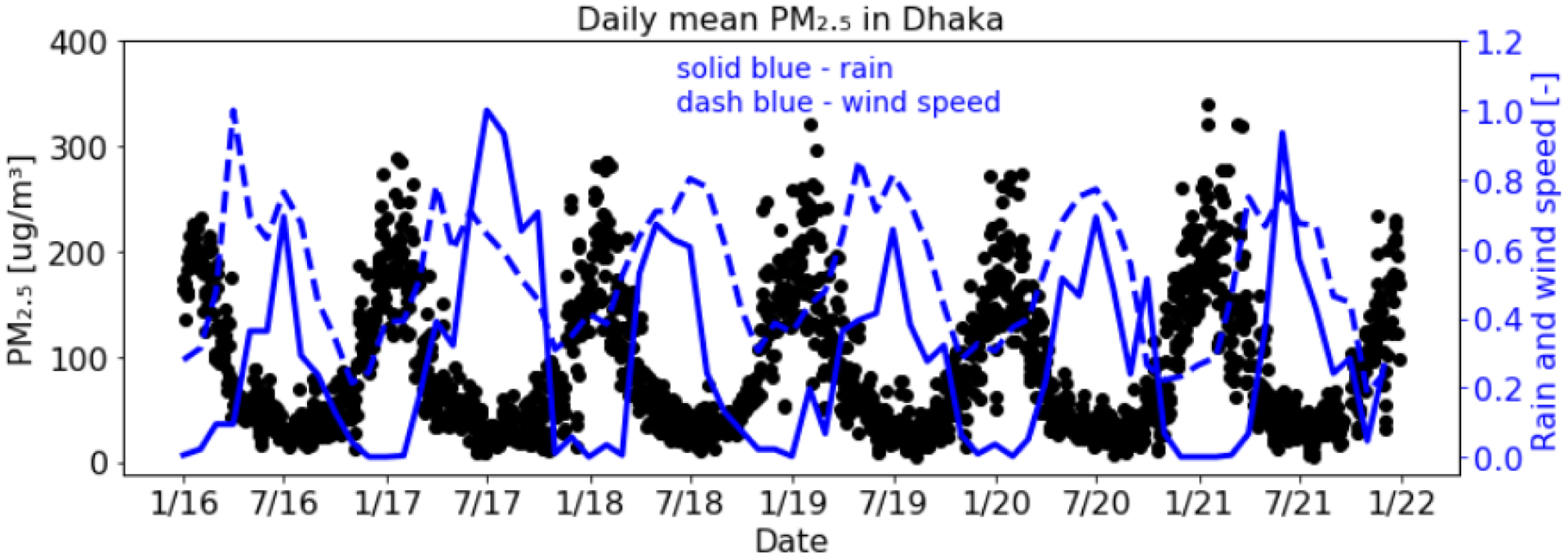
Time series of measured daily-mean PM_2.5 concentrations, normalized monthly total rainfall and normalized monthly mean wind speed from January 1, 2016 to December, 31, 2021. Normalized quantities are calculated by dividing by the maximum monthly values.

3.2. Seasonal, monthly, and annual mean concentrations, exceedances, and pollution episodes

Mean winter PM_2.5 concentration is the highest while the mean monsoon concentration is lowest in each year [Figure 2(a)]. Mean pre-monsoon and post-monsoon PM_2.5 concentrations fall between winter and monsoon concentrations. Seasonal mean PM_2.5 concentrations exhibit negligible inter-annual variability with winter PM_2.5 concentrations of ~165–175 μg/m³ and monsoon concentrations of ~30–35 μg/m³. Thus, the mean winter concentrations are ~5 times greater than those during the monsoon season. The resulting annual mean PM_2.5 concentrations are high ( ~79.7–98.0 μg/m³); 5–6 times greater than the Bangladesh annual ambient PM_2.5 standard of 15 μg/m³, and 6–8 times higher than the U.S. annual PM_2.5 standard of 12 μg/m³. Mean concentrations for all seasons are greater than the annual PM_2.5 standard in Bangladesh (15 μg/m³). Seasonal mean concentrations in winter, pre-monsoon, and post-monsoon are also greater than the daily PM_2.5 standard in Bangladesh. Only the mean monsoon season concentration is lower than the daily PM_2.5 standard in Bangladesh.

Figure 2:

(a) Annual and seasonal mean PM_2.5 concentrations (b) maximum and minimum monthly mean PM_2.5 concentrations (c) number of days exceeding the daily PM_2.5 standard in Bangladesh, and (d) pollution episodes and the maximum duration of pollution episodes during 2016–2021.

The highest monthly mean concentration ranged between 180–210 μg/m³ and always occurred in January [Figure 2(b)]. In contrast, the lowest monthly mean concentration ranged between 26–30 μg/m³ and occurred in July or August. The monthly mean concentration in January can be ~7 times greater than the lowest monthly mean concentration. The number of days exceeding the daily PM_2.5 standard in Bangladesh in a year varied between 144–188 [Figure 2(c)], with the highest number occurring in winter and the lowest in monsoon seasons. In some years, more than 50% of the days exceeded the daily PM_2.5 standard in Bangladesh. The number of pollution episodes varied between 7–11 per year [Figure 2(d)]. We define a pollution episode as a period in which the daily-mean PM_2.5 concentrations remained higher than 65 μg/m³ for 3 consecutive days or longer. The maximum duration of a pollution episode in each year varied between 57–87 days. PM_2.5 concentrations in January-March remain high which contributes to persistent, prolonged pollution episodes each year. Since in our analysis we constrained the data by calendar year, the maximum duration of a pollution episode depicted in Figure 2(d) is somewhat lower. If the analysis was extended to include consecutive months in the cool season (November through February), then the maximum duration of a pollution episode would have been 112 days.

We compare our annual mean PM_2.5 concentrations to the previously reported measurements using similar methods in Figure S.3. The Department of Environment in Bangladesh operates a continuous monitoring station in Dhaka and measures atmospheric PM_2.5 concentrations. Motalib and Lasco (2013) reported annual mean PM_2.5 concentrations of 69.1–89.5 μg/m³ for the years of 2002–2010. Rana and Biswas (2018) reported annual mean concentrations of 68.0–95.0 μg/m³ for the years of 2013–2017. Data capture rates were greater than 85% for all years except 2016 in which data capture rate was only 64%. Thus, we do not use the reported 2016 annual mean concentration for this analysis and replace it by using the average of 2015 and 2017 measured annual concentrations. The annual mean concentration ranges between 69.1–98.0 μg/m³ with the lowest value occuring in 2002 and the highest in 2021 (Figure S.3). The concentration changes from year to year due to variation in emissions, meteorological factors, and long-range transport and has a slight increasing trend.

3.3. Diurnal variation of observed PM_2.5 concentrations

Seasonal mean diurnal profiles of PM_2.5 concentrations were calculated using data for 2016–2021 (Figure 3). As expected, winter concentrations are the highest and monsoon concentrations are the lowest. Concentrations in pre- and post-monsoon seasons remain between the monsoon and winter seasons. Similar to the findings of Mahmood et al. (2019), we find that night-time concentrations are greater than daytime concentrations. And consistent with the findings of Faisal et al. (2022), we find a small morning increase in the diurnal concentrations. In winter, the highest night-time concentration was 2.1 times higher than the lowest daytime concentration. Similar variability in day and night values were observed in other seasons. However, the magnitude of such difference was the lowest in monsoon. Seasonal mean diurnal PBL heights and wind speeds from WRF show distinct seasonal differences (Figure 3). Expectedly, night-time PBL heights in winter are the lowest among all seasons. Wind speeds in winter are also lower than those in pre-monsoon and monsoon seasons. Scant rainfall, low wind speed, and the shallow night-time PBL height contribute to the winter night-time having the highest concentrations. Azkar et al. (2012) reported that heavy-duty diesel vehicles operate only at night in Dhaka releasing additional emissions and further increasing night-time concentration. Daytime PBL height in winter is the second highest among all seasons, significantly reducing daytime concentration and causing a large difference between night and daytime concentrations. In contrast, abundant rainfall and higher wind speed keep concentrations low during monsoon season. Daytime PBL heights in monsoon are the lowest among the seasons which keep daytime concentrations higher than the values that would have existed with higher day-time PBL heights. Such dynamics keeps the diurnal range of concentrations smaller in monsoon than in other seasons.

Figure 3:

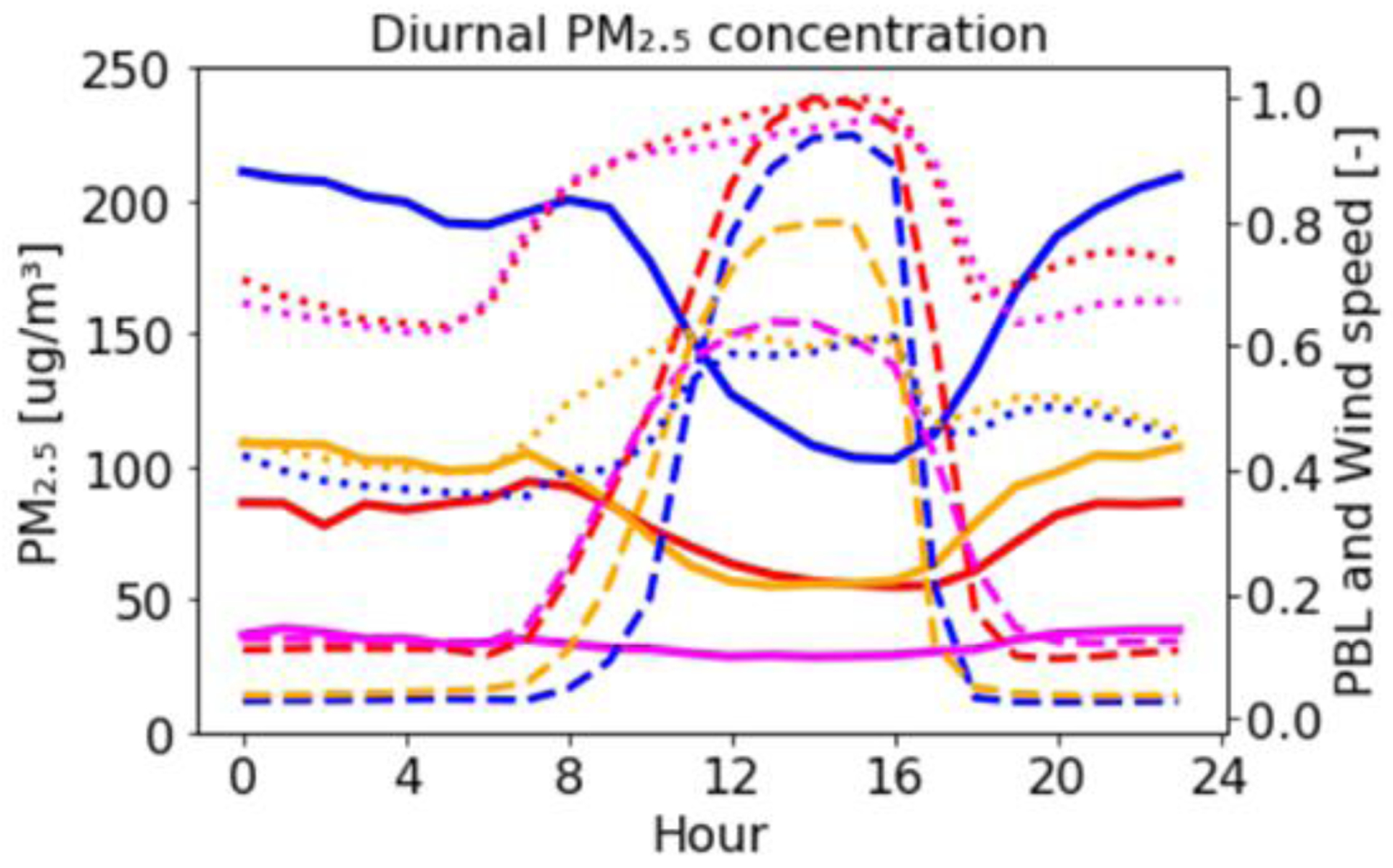
Seasonal mean diurnal observed PM_2.5 concentrations (solid lines) along with seasonal mean Planetary Boundary Layers (dashed lines) and wind speeds (dotted lines) from the WRF model. PBL and wind speeds have been normalized by their maximum values. Blue color represents winter, orange color represents post-monsoon, red color represents pre-monsoon, and magenta color represents monsoon seasons. Hour refers to local standard time.

3.4. Variation of weekday and weekend concentrations

We calculated seasonal mean weekday (Sunday-Thursday) and weekend (Friday-Saturday) PM_2.5 concentrations using all data and find that weekday concentrations are greater than the weekend concentrations in each season. Such results are consistent with the findings of Salam et al. (2012), who also reported that weekday concentrations are higher due to more traffic on weekdays. However, we find weekday and weekend differences are small and did not exhibit a consistent directionality for individual years, possibly due to the confounding effects of synoptic-scale meteorological variability affecting these differences over shorter time periods (Pierce et al., 2010). For example, seasonal mean weekday concentrations are higher by only 1–2 μg/m³ (1–5%) than the weekend concentrations when we used all data from 6 years. When we analyzed the data on a yearly basis, we found annual mean weekday concentrations are higher by 3–8 μg/m³ (3–9%) than weekend concentrations in 2017, 2018, 2020, and 2021. However, annual mean weekday concentrations are lower than weekend concentrations in 2016 and 2019 by 2–4 μg/m³ (3–5%).

4.0. Analysis of CMAQ results

4.1. Comparison of CMAQ predictions with observed monthly mean PM_2.5 concentrations

CMAQ-predicted monthly mean PM_2.5 concentrations for 2017 are compared to observed data in Figure 4(a). Observed data follow the seasonal trend of the highest concentrations in winter and the lowest concentrations in monsoon months. The model captures the monthly variability in observed PM_2.5 concentrations well; however, it under-predicts PM_2.5 concentrations in January, February, and December with a Normalized Mean Bias (NMB, Eder and Yu, 2006) of 13–32%. The model predictions compare well with observed PM_2.5 in other months. Azkar et al. (2012) applied the CMAQv4.7 model over Bangladesh for two winter months (January 2004 and January 2007) using meteorological fields generated from the WRF model and emissions from the Regional Emission Inventory in Asia (REAS) (Ohara et al., 2007). They reported that the model substantially under-predicted observed PM_2.5 concentrations and attributed such underprediction to the missing emissions for brick kilns and resuspended road dust in REAS and the missing wind-blown dust in CMAQv4.7. They performed additional model simulations using two different estimates for brick kilns emissions: one using the USEPA AP-42 factors and the other using the local emissions factor. The model with brick kiln emissions estimated with AP-42 factors increased PM_2.5 by a small margin. However, the model with brick kiln emissions estimated with local factors increased PM_2.5 by a large margin, sometimes exceeding observed concentrations. They report that brick kiln emissions can contribute between 15–60% of wintertime PM_2.5 in Dhaka which indicate that brick-kiln emissions may need to be revised in HTAP emission inventories. The missing brick-kiln and resuspended road dust emissions in CMAQ likely contribute to the under-estimation of model PM_2.5 in winter. The coarse grid resolution used in this study distributes emissions over large grid cells and may dilute localized high emissions. Models with finer grid resolution are likely to produce higher localized emissions in some areas, which in turn may lead to spatial gradients in local contributions and total predictions near these hotspots. The long-range transport is likely to be less affected, which means that transport fraction near hotspots could be lower. Models with coarse grid resolution cannot resolve localized hot spots. Future studies with finer grid resolution are needed to better understand the impact of grid resolution on model results.

Figure 4:

(a) A comparison of CMAQ predicted monthly mean PM_2.5 concentrations with observed data (b) a comparison of CMAQ predicted diurnal PM_2.5 concentrations with observed data (c) CMAQ predicted seasonal mean PM_2.5 composition, and (d) CMAQ predicted monthly mean POC, SOC, and OC concentrations. The black dot in Figure 5(d) represents the OC measurement reported by Salam et al. (2021) during November 2013 - February, 2014. Figure (a) includes standard deviation calculated using all available daily observed and model data in a month. Model and observed PM_2.5 values are shown on the left y-axis and NMB values are shown on the right y-axis, and the horizontal dashed line in Figure (a) represents 0 NMB. Figure (b) includes standard deviation calculated using all available hourly observed and model data. OA = organic aerosol, ${\text{SO}}_4^{2-}$= sulfate, ${\text{NO}}_3^{-}$ = nitrate, ${\text{NH}}_4^{+}$ = ammonium, OTHER = un-speciated PM_2.5, EC = elemental carbon, POC = primary organic carbon, SOC = secondary organic carbon, OC = organic carbon.

4.2. Comparison of CMAQ predictions with observed diurnal PM_2.5 concentrations

Model and observed diurnal PM_2.5 concentrations for 2017 were calculated using all hourly data for the entire year of 2017 [Figure 4(b)]. The variability in model concentrations is smaller than the observed data due to the under-estimation of PM_2.5 concentrations in winter season. However, the model tracks the observed diurnal pattern and also predicts higher night-time than daytime concentrations. Predicted night-time concentrations tend to be lower than observed data by 4–18% and predicted day-time concentrations tend to be higher than observed data by 2–16%. In general, the model captures the observed diurnal trend well.

4.3. CMAQ predicted PM_2.5 composition

The seasonal composition of model predicted PM_2.5 is presented in Figure 4(c). The model suggests that OA is the largest component of PM_2.5 in all seasons accounting for more than 55% of PM_2.5 mass. The second-largest contributing species depends on the season. In pre-monsoon and monsoon seasons, sulfate is the second-largest contributor. However, nitrate becomes the second-largest contributor in post-monsoon and winter seasons. More clouds are present in pre-monsoon and monsoon seasons than in post-monsoon and winter seasons (Rana et al., 2016a). The presence of additional clouds in pre-monsoon and monsoon seasons enhances sulfate production, which in turn increases the percentage of sulfate in PM_2.5 mass. In the post-monsoon and winter seasons, the atmosphere contains fewer clouds, producing less sulfate through aqueous phase reactions and consequently lower SO₄^2- levels. The formation of nitric acid in the model can occur via gas-phase chemical reactions and the heterogeneous hydrolysis of dinitrogen pentoxide. Nitric acid can partition into aerosol nitrate, which is favored during lower temperatures. Temperatures in post-monsoon and winter seasons are lower compared to those in pre-monsoon and monsoon seasons (Azad and Kitada, 1998). Consequently, aerosol nitrate tends to be higher in post-monsoon and winter seasons compared to pre-monsoon and monsoon seasons. ${\mathrm{N}\mathrm{H}}_4^{+}$, OTHER, and EC are the next major components in model-estimated PM_2.5. The contribution of other aerosol components to modeled mean PM_2.5 is small and is not shown in the figure.

Generally, this prediction is consistent with the dominant role of biomass and solid fuel burning emissions in the region. The composition of PM_2.5 in Dhaka is not routinely measured; thus, we cannot directly compare our results with extensive measurements. However, we perform a qualitative comparison of the model-predicted composition with results from several studies. Salam et al. (2003) studied aerosol chemical composition in Dhaka, collecting total suspended particles (TSP) at four locations in Dhaka during March-April of 2001 and analyzing the samples with different techniques to determine aerosol composition in TSP. They reported a mean OC concentration of 45.7 μg/m³, calculated an OA concentration of 73.4 μg/m³, and calculated a sum of all analyzed materials of 151 μg/m³. Thus, OA represented ~49% of measured mass in TSP which is similar to our result. Salam et al. (2021) recently reported the measurements of PM_2.5 and OC in Dhaka during November 6, 2013 to February 1, 2014. Using the mean measured OC concentration during normal days and a value of 1.6 for the OA:OC ratio used by Salam et al. (2003), we estimate a value of ~43% for OA in PM_2.5, which is somewhat lower than our result. If we use the CMAQ estimated value of 2.0 for the OA:OC ratio, then we calculate ~54% of PM_2.5 mass as OA, which is very close to our result. Similar to the findings of Salam et al. (2003) and Salam et al. (2021), our results also reveal that OA is the most abundant component of PM_2.5 in Dhaka. Predicted monthly mean POC, SOC, and OC concentrations are shown in Figure 4(d). Their concentrations follow similar seasonal trend with the highest values occuring in winter and the lowest values in monsoon. Salam et al. (2021) reported a mean OC concentration of 43.1 μg/m³ in Dhaka (represented by the black dot in the figure). CMAQ-predicted mean (January, November, and December) OC concentration of 39.0 μg/m³ is comparable to the reported measurement. The importance of secondary aerosol in Dhaka is clear as the SOC concentration is substantially greater than the POC concentration with annual mean SOC concentration being 3.1 times greater than the corresponding POC concentration. Although not shown in the figure, model annual mean SOA is ~2 times greater than the SOC concentration which emphasizes the significance of multigenerational oxidation products in increasing mass in SOA. Thus, our results are also consistent with the findings of Salam et al. (2021) who reported a dominance of secondary aerosol in Dhaka. A substantial portion of the CMAQ-estimated SOA in these simulations is produced from pcSOA which was parameterized using information derived from vehicle emissions in the U.S.; the suitability of such a parametrization to atmospheric condition in Dhaka is not entirely clear and needs future examination. SOA have been linked to increased cardiorespiratory death rates in the U.S. more than other components in PM_2.5 (Pye et al., 2021). Thus, higher SOA concentration in Dhaka merits a closer examination.

5.0. Transboundary pollution in Bangladesh

Several studies (Rana et al., 2016b; Omni et el., 2017; Rahman et al., 2020) revealed the possible impacts of transboundary pollution in Bangladesh. Rana et al. (2016b) analyzed PM_2.5 concentrations in Dhaka, performed backward trajectories using the Hybrid Single-Particle Lagrangian Integrated Trajectory model, and reported that transboundary pollution can contribute to PM_2.5 pollution in Bangladesh. Rahman et al. (2020) assessed the impact of agricultural-waste burning activities in IGP on PM_2.5 during 2013–2017, and reported that they can contribute 40.2% to PM_2.5 mass in Dhaka. We performed a sensitivity simulation by assigning zero values to all emissions in Bangladesh but keeping the emissions from outside of Bangladesh unchanged. For the sensitivity simulation, we removed the entire emissions in all grid-cells with fractional values of 1.0 for Bangladesh areas using the Detailed Emissions Scaling, Isolation, and Diagnostic (DESID) module in the CMAQ model (Murphy et al., 2021). Emissions in grid-cells with fractional values of less than 1.0 for Bangladesh areas were reduced by multiplying the emissions with the fractional values of the grid-cells containing Bangladesh areas. As an example, this procedure resulted in the reduction of 81,663 tons of un-speciated PM_2.5 (OTHER) emissions in Bangladesh which is more than 71,781 tons of anthropogenic emissions (21% of 341,815 tons of anthropogenic PM_2.5 emissions in Bangladesh is OTHER – see section 2.2). Other sources (fires, dust, etc.) contribute to the additional emissions in the model. The difference between the initial and the sensitivity simulations then quantifies the maximum PM_2.5 reductions possible from reducing Bangladesh emissions. Other techniques for calculating such estimate include partial sensitivity analysis (rather than full zero-out). The result of the zero-out analysis is not identical to that of the partial sensitivity analysis due to the non-linear system (Stein and Alpert, 1993) and should be considered one of several possible estimates. If we calculate the impact of Bangladesh emissions by subtracting the impact of transboundary pollution from the initial CMAQ predicted PM_2.5, then the impact of Bangladesh emissions will be under-estimated since CMAQ underestimates PM_2.5 in winter. Thus, we calculate the impact of Bangladesh emissions by subtracting the transboundary pollution from observed PM_2.5 in Dhaka.

The transboundary PM_2.5 contribution varies by month (Figure 5). The transboundary contribution in January, August, November, and December is lower than that of Bangladesh emissions. However, the contribution of transboundary pollution in other months is similar to or exceeds that of Bangladesh emissions. The contribution of transboundary pollution exceeds or similar to the daily PM_2.5 standard in Bangladesh in February and March. The annual mean contribution of the transboundary pollution is 40.6 μg/m³ and accounts for ~51% of the annual mean observed PM_2.5 in Dhaka with Bangladesh emissions accounting for the remaining ~49%. Our estimate of the relative impact of transboundary pollution on PM_2.5 levels in Dhaka is higher than the finding of Rahman et al. (2020) since our result represents the impact of all outside (of Bangladesh) emissions, not just the impact of agricultural-waste burning activities in the IGP. Using the GAM and the U.S. Embassy data in Dhaka, Fey et al. (2021) reported that local emissions contribute ~60% to measured PM_2.5 in dry months (November-March). We estimate that transboundary pollution contributes ~43% and Bangladesh emissions contribute 57% to the observed PM_2.5 in dry months. Thus, our estimates are also consistent with the findings of Fey et al. (2021). Nevertheless, our results reveal that the annual mean transboundary PM_2.5 contribution exceeds the Bangladesh annual standard. Thus, transboundary pollution is an important contributor to PM_2.5 burden in Dhaka which emphasizes the need for developing a regional approach to an air pollution control strategy for improving air quality.

Figure 5:

Impacts of transboundary pollution and local emissions on monthly mean PM_2.5 concentrations in Dhaka. Transboundary pollution is calculated as model predicted PM_2.5 obtained with zero emissions in Bangladesh but keeping all emissions outside Bangladesh unchanged. The impact of local emissions is calculated by subtracting the transboundary pollution from observed PM_2.5 in Dhaka.

It is plausible that unrealistically high model PM_2.5 concentrations outside Bangladesh can contribute to estimated higher transboundary pollution impacts in Dhaka. To examine such a possibility, we compare CMAQ predictions with observed data from monitoring sites at the U.S. Embassies and Consulates in other countries in the region. CMAQ-predicted PM_2.5 concentrations generally follow the observed variation in Yangon (Rangoon), Myanmar and Colombo, Sri Lanka (Figure S.4) with NMBs of less than ±50% for most months. However, the comparison is mixed in Kathmandu, Nepal and Lahore, Pakistan; the model under-predicts observed data in winter months with NMBs of around −50% but over-predicts in some months with a NMB reaching nearly ~200%. However, such an over-prediction occurs only in September when the transboundary contribution is relatively low. Observed data are not available in Rangoon and Lahore for 2017. Thus, we compare model predictions from the 2019 EQUATES simulation with available observed data in 2019. The model predictions also follow the observed variation in New Delhi, Kolkata, Mumbai, Chennai, and Hyderabad in India (Figure S.5). In New Delhi, the model under-predicts observed PM_2.5 in November with a NMB of −54%, over-predicts in July-September with NMBs of 55–116%, and compares well in other months (NMBs <±50%). In Kolkata, it over-predicts observed data with NMBs of 119–192% in September-October and 27–75% in other months. The model predictions compare well with observed PM_2.5 in Mumbai and Hyderabad but tends to over-predict in Chennai. Given that the model is able to reasonably capture variations in PM_2.5 concentrations at many surrounding locations outside of Bangladesh, the estimated transboundary impacts in Dhaka are considered reasonable estimates. The slightly higher model concentrations than observed data in Kolkata can affect the transboundary pollution impact only by a small margin; hence, transboundary impact in this study may be considered representative of an upper limit.

6.0. Summary and future work

We comprehensively analyzed measured PM_2.5 concentrations at the U.S. Embassy in Dhaka, compared the measurements with the CMAQ model results, and performed an additional sensitivity simulation to examine the impact of transboundary pollution. Night-time levels were consistently higher than day-time values. Highest PM_2.5 concentrations occurred in winter and the lowest in monsoon season, with a resulting annual mean concentration of ~79.7–98.0 μg/m³. Concentrations exceeded the daily PM_2.5 standard in Bangladesh on more than 140 days in any given year. While the model captures the seasonal and diurnal variations of observed concentrations, it underestimates observed PM_2.5 concentrations in winter. Model results suggest that OA is the largest component of PM_2.5 in Dhaka, with SOA playing an important role. Transboundary pollution is significant in Dhaka and contributes more than the annual PM_2.5 standard in Bangladesh. Future effort is needed to incorporate improved emissions estimates and speciation into the model. The POA volatility parameters applied here were developed for nonroad diesel engines in the U.S. and the parameters used to describe pcSOA formation were developed to reduce bias against U.S.-based observations. While it is encouraging that the model captures the high observed OC in Dhaka, future effort is needed to develop and incorporate bottom-up organic aerosol formation pathways consistent with relevant precursors in the region. The model used in this study employed a large horizontal grid. Future studies are needed to employ model with a finer-scale horizontal grid resolution, improved emissions estimates, and organic aerosol estimation related to the region. The updated model can then be used to further examine the elevated PM_2.5 concentration in winter, role of organic aerosols, trans-boundary pollution as well as to explore possible air pollution mitigation strategies in Dhaka. Additional research is needed to better understand the high organic aerosol concentration as well as the impact of transboundary pollution in Bangladesh.