Behavioral economic demand modeling chronology, complexities, and considerations: Much ado about zeros

Abstract

Behavioral economic demand has been shown to have high utility in quantifying the value or consumption of a commodity. Demand describes the relationship between cost and consumption of a commodity, and tends to be curvilinear with consumption approaching zero as the cost increases to a sufficiently high cost to suppress consumption completely. Over a period spanning greater than three decades, behavioral economists have made great strides in the modeling of demand and addressing analytical challenges, although this work is not complete and unresolved challenges remain. The analytical challenges associated with modeling zeros both when they arise as consumption values of zero and when consumption at zero cost is assessed have been a substantial part of this evolution in models. The goals of this methodological review are to provide a historical overview of the major behavioral economic demand models that have been proposed, describe some of the common difficulties with analyzing behavioral economic demand, and discuss general considerations for the analysis of demand. In an environment with evolving and multiple competing analytical practices, we conclude that researchers can maximize scientific rigor by embracing transparency in their analysis choices and employing techniques such as sensitivity analyses to determine if their analysis choices impact the conclusions of their experiments.

1. Introduction

Behavioral economic demand quantifies the relationship between the cost to obtain a commodity and consumption of that commodity (Hursh 1984; Bickel, Green, and Vuchinich 1995). The set of assessment tools and analytical methods that are contained within the umbrella term behavioral economic demand have been shown to have high utility in a wide range of research where quantifying the value or consumption of a commodity is a key component of the research questions (Bickel et al. 2014; Acuff et al. 2020; Zvorsky et al. 2019). The relationship between cost and consumption tends to be curvilinear (i.e., nonlinear) with consumption approaching zero as the cost increases to a sufficiently high cost. A curvilinear relationship poses analytical challenges in describing the relationship accurately and making statistical comparisons among conditions or groups in experiments. Curvilinear and nonlinear relationships tend to be relatively more challenging than linear relationships in part because i) a model can take many different forms and parameters can interact with one another in multiple places in the model and ii) there is no closed-form solution to nonlinear models requiring iterative processes to find best-fit values to describe the data. Over a period spanning greater than three decades, behavioral economists have made great strides in the modeling of demand and addressing analytical challenges, although this work is not complete and unresolved challenges remain.

The goals of this manuscript are to: provide a historical overview of the major behavioral economic demand models that have been proposed to describe and quantify the relationship between cost and consumption (section 2); describe some of the common difficulties with analyzing behavioral economic demand and summarize some of the proposed solutions to these problems (section 3); and propose general recommendations for the analysis of demand in the current environment with multiple competing analysis techniques frequently used by researchers (section 4). These sections are meant to be largely independent of one another, and we invite the reader to skip ahead if only one or two are of interest.

The behavioral economic demand literature contains terms that can present interpretive challenges for those new to the area. Throughout this manuscript, we will use the terms described in Table 1 to describe demand concepts and procedures. Within this table, we have also identified conceptually similar terms that are sometimes used along with a definition that highlights those terms that may have model-dependent interpretations or solutions.

Table 1.

Definitions of behavioral economic demand terminology

Term	Similar Terms	Definition
Cost	Price, Unit Price, Effort	The response cost associated with one unit of the commodity. This can be conceptualized as monetary cost, effort expended, number of responses emitted, or some combination of these.
Consumption		Amount of commodity earned or purchased and consumed at a given cost.
Purchasing		Amount of commodity purchased or earned. Typically equivalent to consumption, but more accurate for hypothetical tasks or tasks where all purchases may not be consumed.
Demand elasticity		The reduction in consumption associated with one unit increase in cost. With a curvilinear demand relationship, elasticity changes as cost increases. Typically derived from fitted model parameters, so interpretation may be model dependent. Additionally, some demand models use more than one free parameter to describe demand elasticity, making interpretation of individual parameters and comparisons of elasticity across conditions difficult.
Change in elasticity	α	Because demand is curvilinear and elasticity is associated with cost, some demand models quantify the rate of change in elasticity as cost increases instead of momentary elasticity values at specific prices. Like modeling of elasticity, this is derived from fitted model parameters, making interpretation model dependent.
Demand intensity	Q0	The consumption associated with minimal cost. This is sometimes assessed directly by measuring consumption at no cost (free), and can also be derived from all of the demand models described herein.
Omax	Max expenditure	The maximum spent or maximum effort (Output) at any price. This can be calculated regardless of model chosen by evaluating the demand curve to find Pmax, and then multiplying Pmax by consumption at Pmax.
Pmax		The cost (Price) at the Omax value. This can be calculated regardless of model chosen by evaluating the curve to determine the point at which the curve has a slope of −1 in log-log space.
Breakpoint		The cost that reduces consumption to zero. This can be determined from the raw data or derived from equations that cross zero consumption. Models based on exponential decay functions never reach zero, and therefore cannot derive breakpoint without estimation algorithms.

2. Summary of Demand Model Development

For more than 30 years, behavioral economists have proposed quantitative models to describe the relationship between price or cost of a commodity and consumption or purchasing of that commodity. As experimenters continued to employ behavioral economic demand modeling in the analysis of their data and find value in these techniques to assess valuation of commodities, a steady stream of new refinements to modeling approaches were proposed. In this section, we characterize notable models in this space in chronological order of their first publication. A quantitative model comparison exercise is beyond the scope of this paper; instead, our goal here is to provide a historical overview of these models and discuss their uses and relative benefits and/or weaknesses in ability to describe a publicly available dataset using standardized methods. Of the commonly assessed demand metrics listed in Table 1, these models primarily differ in their evaluation of elasticity and breakpoint. We will therefore highlight the way each model characterizes elasticity and breakpoint.

2.1. Standardized Model Fitting Procedure

To illustrate the similarities and differences between models of demand, all equations were fit using the mixed-models approach to analyzing demand and publicly available data used in Kaplan et al. (2021). The purpose of this model-fitting exercise was not to provide a thorough comparison of model performance, but instead to illustrate best-fit curves graphically and to highlight some fitting issues that can occur with some models. Briefly, the dataset consisted of an alcohol purchase task that had 17 price points ($0, $0.25, $0.50, $1, $1.50, $2, $3, $4, $5, $6, $7, $8, $9, $10, $15, $20) completed by 1104 participants with a total of 18766 observations. All data were included; no participant data were removed if they displayed non-systematic consumption. The various demand equations were all fit using the same basic approach with one exception that will be described in the sections that describe issues or considerations when fitting different equations of demand. All models were fit in R 4.1.1 (R Core Team 2021) using the packages nls.multstart (Padfield and Matheson 2018), beezdemand (Kaplan et al. 2019), and nlme (Pinheiro et al. 2021). First, a grid search was conducted to find optimal start values by fitting each equation to all the data (i.e., pooled approach). In the grid search, a given model is fit using a wide range of values and then the best performing model is selected. The results of the best model determined by the grid search provides the pooled parameter estimates. Then, the pooled parameter estimates were used as start values for the mixed-effects models. If a model did not converge at a tolerance¹ of 0.001 due to the algorithm becoming “stuck” between a set of values (i.e., tolerance criteria would never be met) the model was fit with a higher (i.e., more relaxed) tolerance. Sometimes, certain iterations resulted in an error which terminated the algorithm entirely (e.g., step having error or back solve error. We refer the reader to Pinheiro et al. 2021 for more details on these errors). If this occurred, the tolerance was relaxed to the convergence of the last successful iteration prior to model termination. If a mixed-effects model was fit with a lower tolerance for a particular equation, the parameter estimates from the higher tolerance model were used as start values for a lower tolerance model and the process repeated until either 0.001 tolerance criteria were reached or until the lowest tolerance achievable based on when the algorithm became “stuck” was reached. Different equations were not directly compared to each other based on different metrics used for model selection, and only issues in model fitting or data considerations will be discussed. For models that required dropping consumption data of zero due to a log transformation requirement, data were simply removed, and no data were replaced with non-zero values² For the Hursh and Silberberg (2008) and Koffarnus et al. (2015) models, the k parameter was set to a constant equivalent to the log₁₀ span of all data retained. All model predictions were transformed to represent raw consumption values rather than scaled predictions to allow for plotting to group and individual data. All models were based on the equations as published and methods to help decrease convergence issues (e.g., estimating parameters in log₁₀ space) were not used. Because we did not estimate parameters in log₁₀ space as in Kaplan et al. (2021) to foster comparisons with the typical way demand models are fit, this was a complete reanalysis of the data. This is because we wanted to show all the models as published, and alterations such as fitting parameters in log₁₀ space with the mixed-effects modelling methods adds additional considerations that are best explored in another manuscript.

The fixed-effects predictions (i.e., estimated group consumption across price) for all models discussed can be found in Figure 1. Different coloration and dashes represent the predictions for different models, and group data are represented as circles for each point of consumption with frequency represented as size. The random-effects predictions for two individual participants can be found in Figure 2. The purpose of this figure is to show which data are dropped for some equations, and how different equations behave when estimating random effects. All random-effects predictions for all models for all 1104 participants can be found in the supplemental material. Because the mixed-effects method of analyzing demand data allows for missing data and fitting irregular data, all participants have predictions for all models of demand.

Figure 1.

Fixed effect predictions from all demand models from the alcohol purchase task used in Kaplan et al. (2021). Y-axis is number of drinks purchased; x-axis is log10 price per drink. All model predictions were transformed to represent raw consumption values rather than scaled predictions to allow for plotting to group data. The size of the data points are representative of the number of participants that purchased that number of drinks at a given price. Larger circles indicate higher frequencies. Y-axis is compressed from 11 to 50 but included to illustrate consumption occurring at higher values. Circles touching the y-axis (i.e., left-most circles) represent consumption at 0 cost. Because values of 0 cannot be plotted on a logarithmic scale, models predicted to 0.0000001 for plotting purposes. The break in the x-axis is meant to approximate price as it approaches 0 to demonstrate predicted consumption near 0. X values left of break span from 0.0000001 to 0.15.

Figure 2.

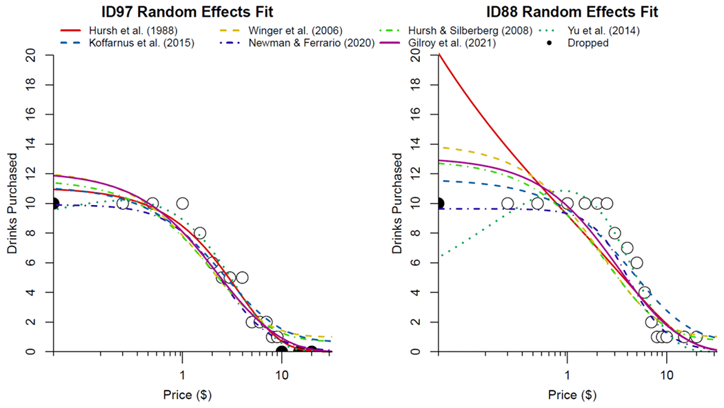
Individual random effects predictions for participants 97 (left panel) and 88 (right panel) to demonstrate similarities and differences between different model predictions based on relatively similar demand data. Y-axis is the number of drinks purchased and x-axis is the log10 price per drink. Points on the that touch the y-axis represent consumption at 0, but the x-axis begins at .05. Filled circles at x values of 0 were removed to fit the Hursh et al. (1988) and Yu et al. (2014) linear elasticity models, while filled circles with y values of 0 were removed to fit the Hursh et al (1988) and Yu et al. (2014) linear elasticity models as well as the Winger et al. (2006) and Hursh and Silberberg (2008) exponential models. Datapoints touching the y-axis (i.e., left-most datapoint) represent consumption at 0 cost. Dropped: Filled circles, represent data that were dropped for some models due to requirements to log-transform price and/or consumption (see text for details). All model predictions were transformed to represent raw consumption values rather than scaled predictions to allow for plotting to individual data.

2.2. Hursh et al., (1988) Linear Elasticity Model

The first model used to describe behavioral-economic demand curves was the linear-elasticity equation, developed by Hursh et al. (1988). This model was the first adaptation of demand modeling from consumer demand theory to the analysis of behavior. The equation,

$$\log Q=\log L+b\left(\log P\right)-aP$$ (1)

describes consumption in relation to price where Q represents daily consumption, P is unit price, L represents the initial level of consumption, and b and a are fitted parameters that characterize the elasticity of demand. The parameter b is the initial downward slope of the demand curve, and a is the acceleration of the slope as the unit price increases.

The linear elasticity model tends to perform well at describing demand data (e.g., Bickel, Madden, and DeGrandpre 1997; Jacobs and Bickel 1999; Hursh et al. 1988). However, it is limited in that there is not one single parameter used to describe elasticity, making interpretation of relative changes in these parameters across groups or conditions difficult. As it is based on an exponential decay function, it also cannot directly evaluate the breakpoint as the curve never crosses or reaches zero consumption, just approaches zero as cost approaches infinity. Another disadvantage of this model is that it cannot innately incorporate consumption values of zero as the log-transformed consumption is modeled, although the exponentiated version of this model proposed by Yu et al. (2014) addresses this issue (see section 2.6.1). This model also sometimes suggests that consumption increases with increases in price, even if this is not evident in the raw data (Figure 1).

When fitted to our example dataset (Figure 1), this model required dropping prices of 0 because x (cost) is log-transformed in the equation, as well as removal of consumption values of 0 for the same reason. There were 1068 (96.7%) participants and 11881 (63.3%) datapoints retained following the removal of 0s. Initial fitting for the mixed-effects model was difficult, as the algorithm would abort following two iterations, and a very high tolerance was required to get initial estimates to use the decreasing tolerance method as described above.

2.3. Winger et al., (2006) Exponential Decay Model

The next model proposed was one based on an exponential decay function adapted for the analysis of demand data (Winger et al. 2006). This equation,

$$\log Q=\log L{e}^{-aP}$$ (2)

models consumption relative to price where Q is consumption, L is maximum consumption at unit price 1.0, P is price, and a is the change in elasticity as a function of price. This model was initially used to describe log-transformed ‘normalized’ data, which is consumption data that has been first transformed to a percentage of maximum consumption, and then log transformed.

Advantages of this model include that it is relatively simple and change in elasticity is modeled as a single free parameter (a), aiding in interpretation of this demand metric. It also describes normalized data well as it inherently assumes that consumption will span two log₁₀ units, matching normalized data ranging from 100% to 1% of maximum consumption. However, this inherent span suited to normalized data can result in poor fits for non-normalized data or failures to converge. Additionally, like with the Hursh et al. (1988) model, log-transformed consumption data are modeled, which results in this model being unable to incorporate zero-levels of consumption without modification. As it is based on an exponential decay function that never reaches zero, breakpoint also cannot be modeled directly.

When fitted to our example dataset (Figure 1), this model required dropping consumption values of 0 because consumption is log-transformed. There were 1094 (99.1%) participants and 12894 (68.7%) datapoints remaining after consumption values of zero were removed. There were no issues with convergence for this equation using our procedures.

2.4. Hursh and Silberberg (2008) Exponential Model

In 2008, Hursh and Silberberg proposed a more generalizable and flexible extension of the exponential decay model that retained the general shape of an exponential decay function, but included additional parameters to accommodate more data patterns:

$$\log Q=\log Q_0+k(e^{-\alpha Q_{0}C}-1)$$ (3)

This model incorporates single parameters representing unconstrained consumption ($Q_0$) and change in elasticity ($\alpha$), respectively. In this model, Q is consumption, k is a constant that specifies the logarithmic range of the consumption data, and C is the price of the commodity. The characteristic of this model to include a single fitted parameter representing demand intensity ($Q_0$) and change in demand elasticity ($\alpha$) is an attractive feature of this model that aids in interpretation of results by allowing researchers to directly interpret model results in terms of useful demand metrics. Note that elasticity is only interpretable as a single free parameter if k is set to a constant as $\alpha$ is not independent of k. If k is allowed to be fit as a free parameter, a summary term incorporating both $\alpha$ and k must be used (Hursh and Roma 2016). Like the previous models, it is based on an exponential decay function, precluding the direct modeling of breakpoint. This model is among the most utilized models of demand, which itself confers some advantages when comparing new research results to previous findings Using a uniform model across research makes it easier to compare parameter values and evaluate trends in the data without having to estimate the influence of model-specific interpretations within reported results.

This model has been used successfully to describe demand across a wide range of datasets, including different contexts (e.g., substance use; “green” product purchases), procedures (e.g., hypothetical and real purchase tasks; laboratory manipulation of fixed-ratio schedules), and species (e.g., humans, rhesus monkeys) (e.g., Yoon et al. 2020; Kaplan, Gelino, and Reed 2018; Koffarnus, Hall, and Winger 2012; Koffarnus, Wilson, and Bickel 2015; Koffarnus and Winger 2015). Despite its advantages, the exponential model is limited in that the fitting of the k value can sometimes produce poor model fits or nonconvergence. This can be avoided by setting k to a constant across datasets, but a shared k value does not always produce good fits for all data. That is, the k value may represent the span of the data for one condition, species, or procedure, but may not represent the span of data for a different condition, species, or procedure. Additionally, the rate of change parameter ($\alpha$) is bounded to the k parameter, making it difficult to compare rate of change in elasticity across experiments (Gilroy, Kaplan, and Reed 2020).

An additional limitation to the exponential model is that it cannot incorporate zeros as published. Because the model is designed to fit log-transformed consumption values, it cannot incorporate consumption values of zero (the logarithm of zero is undefined). This can present analytic problems as consumption values of zero are common in many contexts, and replacing zeros with nonzero values prior to log transformation is also problematic (Strickland et al. 2016; Koffarnus et al. 2015; Yu et al. 2014).

When fitted to our example dataset (Figure 1), this model required dropping consumption values of 0 because this parameter is log-transformed. There were 1094 (99.1%) participants and 12894 (68.7%) datapoints remaining after consumption values of zero were removed. There were no issues with convergence for this equation using our procedures.

2.5. Variations of the Hursh and Silberberg (2008) Exponential Model

2.5.1. Liao et al. (2013) Left-Censored Mixed Effects Model

The left-censored mixed effects model proposed by Liao et al. (2013) is a two-component model where zero values are treated as values below some threshold or limit of detection (i.e., left-censoring). That is, the model assumes that a participant who reports zero might actually be willing to purchase some fractional quantity or amount of the good. This threshold is specified a priori (e.g., .5 units). There are two disadvantages of this equation. One, fitting censored models is somewhat more difficult than non-censored models using statistical programs (Liao et al. use SAS; SAS Institute Inc., Cary, North Carolina). Two, it may be conceptually erroneous to assume that all of a given participant’s reported zero values are actually some fractional quantity greater than zero, but less than one. Rather, it might actually be the case that zero values beyond breakpoint indicate the participant would not purchase any fractional quantity.

2.5.2. Zhao et al. (2016) Two-part Mixed Effects Model

The two-part mixed effects model is a hurdle model and is composed of two parts. The first part of the model relies on modeling zero consumption values using logistic regression. Logistic regression is a popular technique to model binary outcomes, in this case whether or not consumption is zero. The second part reflects the functional form of the exponential model and is applied to positive consumption values only. Conceptually, this model is built on the assumption that zero consumption is indicative of abstinence (as this model was applied to data from a cigarette purchase task). The logistic regression part, therefore, results in a “derived breakpoint,” reflecting the price at which a participant is more likely to report zero consumption (i.e., abstinence) than to report some amount of consumption (positive values).

2.5.3. Ho et al., 2018 Bayesian Hierarchical Model

Although not a different functional model, we highlight a paper by Ho et al. (2018) in which the authors adapted the exponential model to a Bayesian hierarchical model. As discussed earlier in the paper, demand curves have been and are most often analyzed using a nonlinear least squares method whereby coefficients are estimated by minimizing the residual sum of squares or the distance between the model predictions and the observed data. Extending the nonlinear least squares method is the mixed-effects modeling approach, which uses maximum likelihood estimation. Maximum likelihood estimation estimates coefficient values by finding a set of parameter values that is associated with the highest likelihood of observing the actual data. Ho et al. (2018) determine the coefficients using a Bayesian model via Markov Chain Monte Carlo (MCMC) methods. Maximum likelihood is more generally useful than least squares in the sense that optimization of parameters occurs with respect to probability distribution, whereas least squares searches for parameters that minimize the sum of squared residuals. Maximum likelihood is more appropriate for multi-level models, categorical data analysis (including the logistic regression in the previous section), and a wide range of other statistical models that are more complex than the continuous single-level outcome where least squares is appropriate.

In a highly simplified explanation of Bayesian methods, prior distributions are specified for unknown demand parameters, these are combined with the likelihood function (which connects observed data and unknown parameters in a probabilistic sense) and a sampling algorithm is used to obtain a posterior distribution of the unknown parameters given the observed data. All subsequent inference is based on the posterior distribution. A behavioral economic researcher might prefer a Bayesian analysis (i) since the use of MCMC can potentially sidestep optimization issues encountered in nonlinear least squares (e.g., least squares) and mixed-effects (e.g., maximum likelihood estimation) modeling approaches, (ii) to formally incorporate known prior information (for example from previous data analysis or elicited expert opinion (O’Hagan et al. 2006) into the analysis), or (iii) because the interpretations of Bayesian model comparisons and interval estimates are generally more intuitive than frequentist counterparts (see (Franck et al. 2019) for further discussion of this last point using delay discounting case studies) .

2.6. Exponentiations of Previously Described Models

The inability to fit untransformed consumption values of zero is not an inherent limitation of any of the models proposed to this point, but a result of arranging the parameters to operate in logarithmic space. Exponentiation obviates the need to remove zeros or impute nonzero values to replace zeros in datasets. Algebraically rearranging the parameters of any of these equations by exponentiating both sides of them can allow them to fit values in linear space, resulting in the ability to fit untransformed consumption values of zero. A common practice in the demand literature when consumption values of zero are present has been to modify or transform the consumption values in some way to remove any zeros. In Figure 3, we illustrate why these transformations are problematic conceptually, and multiple previous papers have demonstrated these issues with actual participant data and simulated data (Koffarnus et al. 2015; Strickland et al. 2016; Yu et al. 2014). The linear and logarithmic number scales, as do most number scales, share the characteristic that a constant operation representing a change in quantity is applied at each interval of the number scale. With the axes chosen on Figure 3, this is represented by a straight diagonal line. On a linear scale, each increment indicates one additional item, while on a logarithmic number scale each increment on the scale indicates a constant proportional increase in quantity, with that proportional increase represented by the base of the logarithm. That is, both linear and logarithmic number scales are internally consistent across the number line. The difference between 0.1 and 1.1 is the same quantity in the case of a linear scale (1.1 − 0.1 = 1) and same proportion in the case of a base-10 logarithmic scale ([log₁₀(12.589)=1.1]/[log₁₀(1.2589)=0.1] = [log₁₀(10)=1]) as is the difference between 3 and 4 on a linear scale (4 − 3 = 1) and proportion on a base-10 logarithmic scale ([log₁₀(10000)=4]/[log₁₀(1000)=3] = [log₁₀(10)=1]). Common methods of transforming or interpolating demand data to model consumption values of zero with models that require log transformation include: 1) replacing zeros with a nonzero constant prior to log transformation, 2) adding a nonzero constant to all consumption values prior to log transformation, 3) transformation of consumption values to the Inverse Hyperbolic Sine number scale. Each of these methods destroys the internally consistent nature of the number scale, in that all values below a cutoff value are set to or approach a constant, represented visually in Figure 3 as a ‘bending’ of the number line as consumption approaches zero. By ‘bending’ the number line, each of these transformation methods do not share the characteristic that a difference between 0.1 and 1.1 is a constant shift in value (in terms of quantity or proportion) as between 3 and 4. We refer readers to our previous paper (Koffarnus et al. 2015) as well as Yu et al. (2014) and Strickland et al. (2016) for additional discussion and examples of the issues with these transformation and interpolation methods. In sum, each of these methods can be associated with substantial alterations in resulting fitted parameter values, and is inaccurate in simulations where the true fitted parameter values are known.

Figure 3.

Transformed number scales that have been proposed to replace consumption values of zero to be fit with nonlinear regression models that fit log-transformed consumption values compared to log10 transformation as the reference diagonal (orange). Each transformation method involves a ‘bending’ of the number scale compared to the logarithmic scale to create a lower asymptote as untransformed values approach zero. Exponentiated equations (Yu et al. 2014; Koffarnus et al. 2015) and other models designed to fit observed data (Newman & Ferrario 2020) can fit zero values without transformation.

2.6.1. Yu et al. (2014) Exponentiated Linear Elasticity Model

In 2014, Yu and colleagues reported on a modification of the Hursh et al. (1988) model to fit non-log-transformed data. In their manuscript, they describe the issues associated with removing or replacing consumption values of zero in demand experiments, and note that exponentiation of the Hursh et al. 1988 model would allow for the fitting on untransformed consumption values including zeros. The equation is equivalent to the Hursh et al. (1988) model, but solved for untransformed consumption (Q) instead of log(Q), thereby allowing for the fitting of zeros:

$$Q=L\ast P^b\ast e^{-aP}$$ (4)

The authors of this model argue that this model expression is preferable to the originally published version, largely for its ability to fit unmodified consumption values including zeros. The exponentiated equation preserves the interpretive qualities of the original equation, and is generally an improvement to that equation.

When fitted to our example dataset (Figure 1), this model can be run with all consumption values remaining in the dataset, but all predictions of consumption when price is 0 result in 0 or infinity, necessitating the removal of zero-price consumption values and resulting in a dataset of 17662 (94.1%) points. To verify the results, running the mixed-effects model with the full dataset or a dataset with prices of zero dropped yielded the same predictions and outcomes. That is, when running the mixed-effects model with all the data, responses at a price of 0 were dropped automatically. On the second iteration the fitting algorithm aborted, requiring a higher tolerance than 0.001. Using a tolerance of 0.8, the model converged.

2.6.2. Koffarnus et al. (2015) Exponentiated Exponential Model

In 2015, we published on the utility of exponentiated the Hursh and Silberberg (2008) demand model to allow it to model consumption values of zero. Here, we will focus on a brief overview of the benefits and drawbacks of this exponentiated expression of the Hursh and Silberberg (2008) model along with some additional clarifications. Similar to how the Yu et al. (2014) model is a rearrangement of the terms of the Hursh et al. (1988), our 2015 model is simply a rearrangement of the terms of the Hursh and Silberberg (2008) model. Therefore, these two equations are the exact same regression function with the same relationship among the fitted parameters and other model terms, but the equation is solved for observed consumption values instead of log-transformed consumption:

$$Q=Q_0\ast {10}^{k(e^{-\alpha Q_{0}C}-1)}$$ (5)

Solving for and fitting observed consumption can impact how error variance is handled in the fitting process, but does not change the form of the demand equation or the scale or interpretation of the fitted parameters. It does allow for the fitting of untransformed consumption values including zeros, however. To demonstrate that these equations are equivalent in scale and interpretation of variables, we generated a series of idealized datasets based on the assumptions of Hursh and Silberberg (2008). For a range of fitted parameters, we generated the exact consumption values across a series of 19 prices that would be predicted from those parameters according to the Hursh and Silberberg (2008) model. We then took those consumption values and fit them with standard nonlinear regression settings of GraphPad Prism 9. The resulting fitted parameters when fit with Hursh and Silberberg (2008) are identical to a precision of 8 decimal places to the source values, as would be expected with idealized consumption values exactly matching the assumptions of this demand model (Table 2). However, when we converted these same consumption values generated with Hursh and Silberberg (2008) to their non-log-transformed counterparts and fit these newly scaled consumption values with our Koffarnus et al. (2015) exponentiated model, the nonlinear regression fitted parameters are identical to the same 8 decimal place precision as the Hursh and Silberberg (2008) model (Table 2). This was by design so that the exponentiated equation would inherit the benefits of the Hursh and Silberberg model, including the ease in interpretation of the two fitted parameters representing demand intensity and change in demand elasticity, as well as the ability to easily compare results with those previously obtained by others.

Table 2.

Exact consumption values were generated from the test parameters listed below, and were then fit to Hursh and Silberberg (2008) and Koffarnus et al. (2015) using nonlinear regression. The resulting fitted values exactly match the test parameters for both models, reflecting the fact that these two models are equivalent

Test Parameters				Hursh & Silberberg (2008) fitted values				Koffarnus et al. (2015) fitted values
no.	α	Q0	k	Q0	α	k	R2	Q0	α	k	R2
1	0.0001	100	3	100.00	0.0001	3.00	1.00	100.00	0.0001	3.00	1.00
2	0.0001	100	2	100.00	0.0001	2.00	1.00	100.00	0.0001	2.00	1.00
3	0.0001	10	3	10.00	0.0001	3.00	1.00	10.00	0.0001	3.00	1.00
4	0.0001	10	2	10.00	0.0001	2.00	1.00	10.00	0.0001	2.00	1.00
5	0.001	100	3	100.00	0.001	3.00	1.00	100.00	0.001	3.00	1.00
6	0.001	100	2	100.00	0.001	2.00	1.00	100.00	0.001	2.00	1.00
7	0.001	10	3	10.00	0.001	3.00	1.00	10.00	0.001	3.00	1.00
8	0.001	10	2	10.00	0.001	2.00	1.00	10.00	0.001	2.00	1.00
9	0.01	100	3	100.00	0.01	3.00	1.00	100.00	0.01	3.00	1.00
10	0.01	100	2	100.00	0.01	2.00	1.00	100.00	0.01	2.00	1.00
11	0.01	10	3	10.00	0.01	3.00	1.00	10.00	0.01	3.00	1.00
12	0.01	10	2	10.00	0.01	2.00	1.00	10.00	0.01	2.00	1.00

While the Koffarnus et al. (2015) model maintains the same parameter interpretation as the Hursh and Silberberg (2008) model, nonlinear regression optimization algorithms are affected differently by deviations from idealized data when those data are analyzed on a linear scale versus a log-transformed scale. Therefore, for experimentally obtained data that does not conform exactly to the assumptions of these models, the two can generate somewhat different fitted values. In our original paper, we demonstrated that the fits with our exponentiated version are more likely to reproduce independently assessed Q0 values and both Q0 and a values from simulated data where the original true values are known. . In our paper (see Figures 2 and 4 of Koffarnus et al. 2015) and in a systematic replication conducted by others (see Figure 2 of Strickland et al. 2016), the exponentiated equation performed much better with datasets However, as discussed above, nonlinear regression optimization is complicated and it is not obvious whether log or linear scales will produce more ‘correct’ results for any given dataset. This determination is complicated further by the tendency for consumption data to be positively skewed, sometimes to a very high degree. The log transformation employed inherently in the Hursh and Silberberg (2008) equation can alleviate some of this positive skew, but this can also be addressed to some degree in the exponentiated model by fitting log(Q₀) and log(α) values directly. This modification does not alter the interpretation of scale of the parameters, it just optimizes the fits of the log-transformed parameters in log-transformed space. See Kaplan et al. (2021) for more detail on this manipulation.

When fitted to our example dataset (Figure 1), this model did not generate any errors, but got “stuck” between multiple best-fit parameter values when the algorithm was attempting to converge. The model converged when the tolerance criterion was set to 0.06, and a lower tolerance was not achieved after using the first mixed-effects model parameters as starts for a second attempt of a mixed-effects model.

2.7. Newman and Ferrario (2020) Model

Recently, Newman and Ferrario (2020) published a demand model meant to address some of the shortcomings of previous models:

$$Q=Q_0{\left[1+{\left(\frac{P}{P_0}\right)}^b\right]}^{-a/b}$$ (6)

Their model has four free parameters, one ($Q_0$) to determine the starting point of the demand curve at minimal price (demand intensity) and three free parameters that influence how consumption decreases with increases in price: (i) $P_{\mathit{0}}$ affecting the price where consumption starts to decline, (ii) a affecting the slope of the decline, and (iii) b affecting the transition to the elastic portion of the curve. With four free parameters, the shape of this equation is more flexible than the others described in this paper, but the form of the equation still assumes that consumption will only decrease with increases in price. Additionally, the rate of decrease in consumption can only be positively accelerating, which yields the restriction that any demand curve drawn with this equation can only have one Pmax value (i.e., there is only one inflection point per curve that can be interpreted as the price associated with maximal expenditures). From a demand modeling standpoint, the lack of a straightforward way to quantify elasticity or change in elasticity is a disadvantage. However, while this function does not yield a single parameter than can be interpreted as elasticity or change in elasticity, the calculation of the other major demand metrics is straightforward with this equation, including Pmax, Omax, $Q_0$, and breakpoint. Indeed, this is the only model discussed here that can directly model breakpoint, as the form of the curve allows it to cross the zero-consumption point. If some combination of $Q_0$, breakpoint, Pmax, and Omax are the primary metrics of interest, this equation can yield those parameters without some of the complexities of the other models presented here. An additional disadvantage includes fitting complications associated with three free parameters to characterize change in consumption as price increases. In practice, we find that this equation has issues with parameter collinearity (i.e., fitting algorithms unable to converge on a set of fitted parameter values as any adjustment to one of the parameters necessitates an adjustment in one or more other parameter, thereby never reaching a single set of best-fit values).

When fitted to our example dataset (Figure 1), this model was challenging to fit as the parameter estimating method described above yielded fixed-effects estimates that did not seem to produce estimates that visually approximated the underlying data. That is, while all other models resulted in an estimated intercept (i.e., $Q_0$) around 6.5, attempting to fit Equation (6) using the procedure described above resulted in an intercept of ~2.5. Also, when using this method, very high tolerance values (i.e., >1.0) were required to avoid the algorithm aborting using our standard procedure described above. However, using starting values that better visually approximated $Q_0$ and $P_0$ while finding starting values for a and b via trial and error, similar $Q_{\mathit{0}}$ estimates to other models were obtained along with being able to converge the model at a lower tolerance of 0.01. Until these better-performing starting values for $P_0$_, a, and b were found, the algorithm would abort within three to four iterations.

2.8. Gilroy et al. (2021) Zero-Bounded Exponential Model

The most recently published demand model is also a variant of Hursh and Silberberg (2008) that is designed to address the inability of the original equation to fit consumption values of zero. The equation appears similar to Hursh and Silberberg (2008), but consumption data are analyzed after transforming to a modified number scale – the Inverse Hyperbolic Sine (IHS) scale – instead of log-transforming the data. The IHS transformation is a nonuniform transformation that closely approximates a log transformation for most of the number scale, but deviates substantially from the standard log scale as untransformed values approach zero. By transforming all positive and zero values to nonzero positive numbers, consumption data on this number scale can be fit with Hursh and Silberberg (2008). The authors’ equation is a solution that completes this data transformation step to the IHS scale and fitting to Hursh and Silberberg (2008) in one step:

$$IHS(Q)=IHS(Q_0)+IHS(Q_0)\ast e^{-\alpha Q_{0}P}-1$$ (7)

$$\text{where}\hspace{0.17em}IHS(Q_0)=lo{g}_{10}\left(0.5\ast Q_0+\sqrt{0.25\ast Q_0{}^2+1}\right)$$

Despite the similarities in appearance and parameter names with Hursh and Silberberg (2008), this equation does not maintain the same interpretation or scale for the fitted parameters, primarily alpha. This is because alpha measures the change in elasticity in IHS units, not the logarithmic units assumed by both Hursh and Silberberg (2008) and Koffarnus et al. (2015). Additionally, as is shown in Figure 3, the IHS number scale is similar to the effective number scale formed when consumption values of zero are replaced with a nonzero number (in this case, 1.0) or when a constant of 1.0 is added to all consumption values prior to log transformation (see Section 2.6). As discussed in Yu et al. (2014), Koffarnus et al. (2015), and Strickland et al. (2016), replacement of zero consumption values with a nonzero constant can have problematic consequences and alter the conclusions drawn from an analysis. The IHS scale is not identical to a number scale where zero values were replaced by 1.0 or when 1.0 is added to all consumption values prior to log transformation as the IHS scale transitions from the log scale to the nonzero replacement constant slightly differently, but the two procedures are similar in how values equal to or below 1.0 are transformed to similar values (see Figure 3 and Section 2.6). Like the other models based on exponential decay functions, this model also cannot directly evaluate the breakpoint as modeled consumption never reaches a true zero point.

When fitted to our example dataset (Figure 1), this model did not have any errors occur, but much like the Koffarnus et al. (2015) model, the fitting algorithm got “stuck” attempting to converge. The model was fit with convergence criterion set to a value of 0.11, and using this change did not result in achieving a lower tolerance.

2.9. Summary of Demand Models

Behavioral economic demand, conceptually, describes consumption patterns across a vast range of commodities and situations. Modeling of this behavior has made great strides, but is ongoing. Existing models have each iterated on previous models or attempted to solve analytical solutions with previous models, but have not yet resulted in a model that is accepted as the “correct” model to be used by all researchers.

3. Complexities Associated with Behavioral Economic Demand Analyses

Contrary to more classical economic paradigms whereby the relation between consumption and price of a commodity is modeled using a linear relationship, the behavioral economic framework has historically used nonlinear regression. Nonlinear regression presumes differential changes in the outcome variable (e.g., consumption) depending on changes in the predictor variable (e.g., price). When prices are small (low, cheap), changes in consumption are small. As price increases, changes (usually decreases) in consumption become larger. Although nonlinear regression techniques are not unique to behavioral economic demand analyses, they do present additional complications and considerations compared to linear regression. We highlight some of the prominent issues that might be encountered when using nonlinear regression and potential mitigating strategies.

In nonlinear regression, estimating the parameter values that best reflect the underlying data is accomplished through an iterative process (Pinheiro and Bates 2006). Partly due to this iterative process, the complexity of contemporary demand equations, and the degree to which a given dataset reflects a typical demand function, misspecification of initial values to begin the iterative process can present issues. If the initial values are too far away from the optimal solution, then the model may fail to converge completely or converge at a “local minimum/maximum” (i.e., a solution that appears to be good enough, but a more optimal solution exists at some other parameter value combination). There are no “silver bullets” to this optimization problem, but some strategies may help. When conducting nonlinear regression, initial values for $Q_0$ (or similar depending on model) compared to other fitted parameters may be easier to determine because usually one can use the observed value at the lowest price as the starting value. Elasticity parameters such as α may be more difficult and may require several different guesses before a model converges.

3.1. Choosing Starting Values

Start values can be determined in several ways. The first is based on experimenter experience (i.e., start values that have worked before). This method is reasonable, but when working with unfamiliar demand data, starts that previously worked may not identify optimal model fits (e.g., starts for the elasticity parameter may vary greatly among drugs or nondrug commodities). The second is by using start values that have been reported in empirical literature, assuming these are available. A third way is using a “grid search” to identify optimal start values. This method involves attempting a predetermined range of start values and choosing the best fitting model that converges based on that range. The grid search method allows for flexibility in novel datasets, although a likely range of values is still required to be provided for the researcher. The issue of choosing optimal start values becomes more important when attempting mixed-effects modelling (Section 3.2), as the increased complexity of the analysis is more likely to lead to issues of nonconvergence. This means the first and second ways of determining start values can be less effective, particularly when using mixed-effects modelling that includes within- or between-subject manipulations. For mixed-effects modelling, every different condition requires a start value that is relative to some reference condition. While further details of determining start values for more complex mixed-effects modelling are outside of the scope of the present manuscript, see Rzeszutek et al. (2022) for a description of determining start values for mixed-effects modelling of demand for multiple within-subject conditions. Because of the ease of use of prebuilt R packages such as nls.multstart (Padfield and Matheson 2018) to conduct grid searches for finding optimal start values, this is currently our preferred method. Note that the grid search method for determining start values technically removes the need for the experimenter to choose optimal start values, and instead allows optimal start values to be found via an algorithm, decreasing issues of non-convergence when using a “two-stage” or mixed-effects modelling approach described below.

3.2. Mixed-Effect Models

As described in Kaplan et al. (2021), there are two common ways of fitting demand curve data. The first is what we have termed the “fit-to-means” approach and is done either by fitting a single curve to all data or by averaging consumption values at each price and then fitting a single curve to those averaged consumption values. The other is the “two-stage” approach where a single curve is fit to each participant’s dataset. Each of these approaches have issues, which are largely mitigated by using a mixed-effects modeling approach. Briefly, the primary issues with the fit-to-means approach are that dependence in the data (e.g., consumption values for a given participant are more similar to their own consumption values as they are to another participant) is ignored (i.e., participant-level parameters are not estimated). A primary issue with the two-stage approach is that regressions in the first stage may be especially difficult to fit to individual subject data that display the irregular data patterns described by (Stein et al. 2015).

3.3. Empirical Data Issues

Demand data are typically characterized by a downwardly sloping trend as price or cost increases (see Figure 1). As with any behavioral task that relies on human participants responding based on experimenter instructions, data resulting from participants may violate the normality assumptions common to nonlinear regression or not be indicative of a theoretically assumed pattern of responding (i.e., non-systematic data). Irregular data patterns that do not conform to the assumptions of the model being fitted typically results in poor model fits, and a common response to this issue is to remove the offending data from the analyzed dataset. This can solve the fitting issues, but also poses problems with biasing results toward the authors’ hypothesis that rely on the same assumptions about data regularity. An advantage of mixed-effect modeling approaches is that all data can be included in a single model, even those data that do not conform to pre-existing hypotheses. Therefore, mixed-effect modeling could be considered a more conservative, agnostic approach that does not presuppose an effect prior to the analysis. Two types of data that appear atypical may be observed. The first type can be considered as consumption values that are far away from other values or far away from some measure of central tendency (e.g., mean, median). The second type is nonsystematic data in which consumption patterns do not meet the prototypical downward sloping trend. We will take these two atypical data patterns in turn.

3.3.1. Outlier consumption values

Consumption values that appear far from what may be expected could be considered “outliers.” We use this term for ease although we recognize that it can be associated with many different definitions. Here, we mean values that seem unusually remote from the trend established by the rest of the observed data, which may give the researcher pause. For example, if a task is asking about how many cigarettes would be purchased for consumption during the next 24 hours, a consumption value of 20 makes sense as there are many smokers who regularly consume this many cigarettes in one day. However, a consumption value of 200 may make little sense and may border on physically impossible to consume in a 24-hour period. Unrealistic or impossible data may arise due to a number of factors, one of which may be participants misunderstanding the instructions provided. On the other hand, a consumption value of 60 – although seemingly far from what may be the average and meeting traditional definitions of an “outlier” – may reflect actual consumption as smokers who consume 60 cigarettes per day do exist, although the number of 60-cigarette-per-day smokers may be relatively low. One relatively conservative method of identifying extreme values is to determine the feasible number of units (e.g., cigarettes, alcohol drinks) a person could possibly consume in the timeframe provided and use that number as a threshold. Any values above this value may warrant exclusion with the reasoning that the participant was responding in a way that reflects a lack of adherence to task instructions, although any data exclusion rules should be identified a priori to avoid instances of unintentional (or intentional) “p hacking”, or performing multiple analyses until one is discovered that conforms to the researcher’s hypothesis. Another method of dealing with extreme values in the literature include winsorizing (Tabachnick and Fidell 2019). Tabachnick and Fidell (2019) suggest “Cases with standardized scores in excess of 3.29 (p < .001, two-tailed test) are potential outliers” (pg. 64) and some researchers have used this value in winsorizing such that any values exceeding 3.29 standard deviations are recoded to the next highest non-outlying value. This approach has been used rather rigidly even though the Tabachnick and Fidell (2019) note “However, the extremeness of a standardized score depends on the size of the sample; with a very large N, a few standardized scores in excess of 3.29 are expected” (pg. 64). In the case of demand data, positively skewed distributions are common, and winsorizing may exclude data that represent the actual range of consumption patterns in a sample. Therefore, winsorizing for demand data should be only used with a strong, empirically supported justification. We refer readers to various reviews from Kaplan et al. (2018) and Reed et al. (2020) who have cataloged the different methods of exclusion.

3.3.2. Irregular Patterns of Consumption Data

Consumption values do not need to be far from the general distribution to be suspect or questioned. The magnitude of consumption values individually may seem perfectly realistic, yet a participant’s pattern of responding may suggest illogical responding, misunderstanding of the task, or inattention. One way researchers have delt with these datasets is by identifying and excluding any response sets that exhibit low goodness of fit values (e.g., R² ≤ .30), suggesting that the model being used does not describe the data well. Because goodness of fit can depend on the analytical decisions such as the model being used and presupposes that the chosen model is the correct description of behavior, some researchers have attempted to standardize the criteria by which a response set is judged to be potentially unsystematic. Three criteria have been proposed by Stein et al. (2015), based on similar criteria for delay discounting data proposed by Bruner and Johnson (2014): 1) trend (a global reduction in consumption from the first price to the last price), 2) bounce (the number of price-to-price increases in excess of 25% of consumption at the lowest price), and 3) reversals from zero (non-zero consumption after two consecutive zero consumption values). These criteria appear to be useful for initial identification of response sets that suggest inattention, inconsistent responding, or misunderstanding of the task. We note – to reiterate Stein and colleagues’ recommendation – these criteria should be used as initial identification and not used to indiscriminately remove or censor data. For example, the trend criterion may only be applicable to commodities where consumption is assumed to be negatively correlated with price. Other goods, such as Veblen goods, do not necessarily carry this assumption (Bagwell and Bernheim 1996). Veblen goods are characterized by a positive relation between demand and price; consumption of these goods increase as price increases. These goods are typically more “exclusive” and carry some sort of status symbol. Another situation in which the trend criterion may not applicable is with null or completely zero consumption. For example, asking cigarette naïve participants or participants who have quit using cigarettes about how many cigarettes they would purchase may result in null demand. This pattern of responding may be valid and these participants should not be excluded from a broader analysis attempting to characterize consumption patterns in a group that includes nonsmokers. Finally, the trend criterion may not be applicable in cases where consumption is insensitive to price. For example, some goods may be necessary (e.g., water) and must be purchased in consistent quantities regardless of price. Whereas these goods may be exceedingly rare, instances may be possible. We recommend researchers clearly identify a rationale when “unsystematic” response sets are or are not retained, and make these inclusion/exclusion judgements prior to data collection.

3.3.3. Empirical Data Issues and Model Fitting

The aforementioned issues with outliers and atypical response sets can cause problems when analyzed using traditional methods of nonlinear regression, to a greater extent when using the two-stage approach and a lesser extent using the fit-to-means approach (Kaplan et al. 2021). Atypical response patterns, when observed in relatively low frequency, are not especially problematic when fitting to either the precalculated averages or to the entire data set because these response patterns are effectively “smoothed” out and do not substantially alter the sample-level trend. Furthermore, inclusion of inconsistent data adds potentially realistic variability to group estimates and tempers any statistical conclusions made, an arguably justified consequence for datasets containing large amounts of irregular data patterns. Extreme values can present more serious issues in the fit-to-means approach, depending on the frequency and magnitude which they occur. When averaging consumption values at each price, each consumption value contributes equal weight to the average. Thus, extreme values in high enough frequency or low frequency but in high enough magnitude may “pull” the averaged consumption values higher or lower than what might be expected if these values were not present. Given consumption values are bounded at zero and typically skewed towards higher values (Fmanegative consumption values are nonsensical for consumption of a positive reinforcer), averaged data is often shifted higher when these extreme values are present. Atypical response patterns – especially null or static consumption – are more problematic when fitting using the two-stage approach. Although some demand models can theoretically produce estimates from “flat-line” consumption patterns, more often these models will fail to converge or result in negative R² values (a valid possibility in the context of nonlinear regression), an indication that the ‘best-fit’ curve does not describe any pattern in the data better than a “noise” model characterized by a horizontal line. Nonconvergence systematically reduces available data for the second-stage analyses (e.g., analysis of variance, t-tests) and may lead to bias and/or standard errors that do not reflect the empirical range of values in the data. This issue is further exacerbated since such data are not missing at random (e.g., in a Cigarette Purchase Task, all of the null demand response sets arise from former cigarette smokers). Outcomes from the second stage of analyses would certainly be biased.

3.3.4. Mixed-Effect Models Can Be Robust to Irregular Data

Both the outlier and atypical response set issues are largely remedied by adopting a mixed-effects model framework for analyses (Kaplan et al. 2021). Briefly, mixed-effects models are able to simultaneously leverage all data at once resulting in a “group-level” curve (describing how the sample as a whole responds) and individual-level predictions (participants are assigned their own demand values for the unknown model parameters). In-depth discussion about the relative merits of mixed-effects modeling is beyond the scope of this paper, but we note that because mixed-effects models leverage all data simultaneously and recognize where the majority of the consumption values lie, parameter predictions associated with participants with extreme values are “shrunk” towards the group-level estimates. Said another way, values that are far from most of the sample are assigned a lower weight and confidence in those values is reduced. Because mixed-effects models do not directly estimate individual parameters (rather, individual predictions arise from modeling a distribution centered around the group-level fixed-effect parameters), they can provide predictions for participants with static consumption. Implementing mixed effects modeling requires some additional technical prowess compared with fit-to-means and two-stage approaches (see Kaplan et al. 2021 for more detail).

One final issue related to modeling demand curve data should be noted. As alluded to earlier, consumption values are bounded at zero and zero demand is frequently observed (whether or not preceded by nonzero consumption). This boundary is a violation of the normality assumptions typically made in the regression framework. Some models support including zero values without alteration and some do not (see section 3). The models that do not support zero values rely on log transforming consumption prior to fitting. Log transforming consumption values results in some favorable attributes such as reducing skewness. However, the primary limitation of log transformations is that the logarithm of zero is undefined and therefore cannot be included in the modeling step without imputation methods that can alter statistical conclusions made (Koffarnus et al. 2015).

3.4. Model Fitting Error and Residuals

Each of the models reviewed in this paper prescribe a decreasing function for demand as a function of cost. Since observed demand data do not fall exactly on the regression line (e.g., see Figure 1), it is necessary to model the departures between the observed data and what is expected based on the line. In statistical parlance, residuals are the differences between observed data and the value of the regression line at a given price. Error variance describes how far the points are from the line by aggregating the squared differences between data and trend line. Small values of error variance correspond to points closely clustered around the line, and larger error variance occurs when points are farther from the line. The default approach to quantifying error variance is to use a normal distribution, and each of the models reviewed in this paper implicitly use a normal distribution assumption to model unexplained variability in data. In practice, the assumption of normally distributed residuals is extremely convenient as methods to fit such models are readily available and optimize relatively easily. In reality, the normality assumption is probably too simplistic as demand data distributions can vary wildly from commodity to commodity and population to population. A direction for future research would be to develop modeling approaches and software infrastructure that (i) applies non-constant variance that, for example, allows error variance to be lower at high prices where consumption is less variable, and (ii) honor the lower bound of zero in consumption. Methods that better characterize the distribution of residuals would provide a more realistic gauge of the uncertainty that exists in observed data. This would lead to confidence intervals and hypothesis tests that more effectively separate signal from noise (since the quantification of noise would be improved). Additionally, any approach that more realistically describes residuals could potentially be useful to inform Monte Carlo simulation studies that would, for example, enable researchers to conduct sample size and power calculations on the basis of models that are used in practice rather than resorting to overly simplified power analyses.

4. General Considerations

The study of demand has been proceeding for decades, with many models proposed that characterize consumption as a function of cost. Section 2 covers many aspects of a number of these models, but a natural question remains: which model(s) should a researcher use when analyzing demand data? Choosing which model to use is ultimately subjective, as there is no notion of a single objectively “best” model. As shown in Figure 1, each of these models visually fits our example dataset in a way that roughly corresponds to the general trend evident in the data. Each of them may function adequately as a descriptive model of data in most experiments. Here, we discuss four relevant considerations which may help the reader make this choice in practice: theoretical appeal, parsimony, ease of use, and interpretability.

Behavioral economic theory generally presumes that consumption of a commodity decreases with increases in cost required to obtain that commodity, and each of the models discussed in this paper formally adopt that assumption and impose that structure on the experimental data. Furthermore, behavioral economists have identified many summary measures that have interpretive and theoretical appeal (see Table 1). A model with high theoretical appeal would allow for the straightforward assessment of as many of these concepts as possible to accommodate experimental questions relating to one or more of these concepts.

A model that is parsimonious satisfies Occam’s razor, since it is the simplest model that adequately describes the data. In this context, models with more parameters are more complex than models with fewer parameters. Additional parameters tend to lead to more flexible curves that can “get closer to” data in terms of good model fits with small residuals. However, models that are too complex risk overfitting the data. Overfitting occurs when models attribute chance variation in the specific data set at hand to meaningful underlying structure, and hence overfit models are not useful for predicting future data.

Statistical information criteria such as Akaike’s Information Criterion (AIC) (Akaike 1998) and Bayesian Information Criterion (BIC) (Schwarz 1978) strive to identify parsimonious models by weighing the likelihood of each competing model against a penalty that is based on complexity. These metrics can be useful to compare models’ performance on a given data set, but they should be interpreted with a few important caveats. First, it is frequently the case that the model with the best statistical metric (e.g. AIC, BIC, adjusted R², etc.) is only barely better than several other competing models. In this case, little evidence is available to decisively discover a single true underlying model, and a replication study might easily result in a different model having the best statistical performance for a new data set. We note that among information criteria, BIC is model selection consistent and thus is increasingly likely to choose the correct model if it is in the candidate set. AIC tends to choose larger models than BIC (Schwarz 1978). Second, statistical metrics operate solely on observed data and thus belie the important role that scientific theory should play in the context of debating models and advancing the field. Despite these caveats, statistical model selection metrics are useful in the sense they provide concrete feedback on the tradeoff between model fit and complexity for specific data that are under analysis.

In addition to choosing with functional form the model should take, the reader also needs to decide whether to pursue a pooled, two-stage, or mixed effects modeling approach to model fitting and inference. We advocate against the pooled analysis, as it does not properly account for within-subject correlation and thus leads to incorrect standard errors and misleading inferences. Generally, the two-stage approach is simpler to implement than the mixed-effects modeling approach (also known as hierarchical modeling), but the mixed-effects approach models group and individual level effects simultaneously and is more elegant (for more information, see Kaplan et al. 2021).

Despite the guidelines outline here, the ultimate choice to use one demand model over the others will likely result in some degree of uncertainty due to the complexities of this decision. As with difficult analysis choices in other contexts, best practices that maximize scientific rigor involve some straightforward principles. First, the analysis protocol should be outlined prior to data collection. Doing so will help prevent “p hacking”, the practice where analysis choices among viable alternatives are influenced (potentially even unintentionally) by the knowledge about which method will produce the lowest p value. Second, sensitivity analyses can be incorporated into the analysis protocol to determine if analysis choices had a substantial impact on conclusions drawn. For example, secondary analyses could be conducted with differing assumptions, methods, or models employed than the pre-determined primary analysis. If the results of these secondary analyses differ substantially from the primary analysis, caveats and tempered language could be included in research reports to indicate that the results may have been affected by those assumptions, methods, or models employed.

5. Conclusions and Future Directions

Behavioral economic demand analyses have been productively used to assess valuation processes in a large and growing set of experiments. Modeling of demand data and best practices for nonlinear analysis techniques are both evolving topics being actively studied. In this changing environment, researchers can maximize scientific rigor by embracing transparency in their analysis choices and employing analysis steps such as sensitivity analyses to determine if their analysis choices impact the conclusions of their experiments. Future research should and likely will continue to improve upon these techniques and establish more streamlined analysis pipelines that are standardized and approachable for new researchers.

References

- Acuff SF, Amlung M, Dennhardt AA, MacKillop J and Murphy JG 2020. Experimental manipulations of behavioral economic demand for addictive commodities: A meta-analysis. Addiction, 115: 817–831. [DOI] [PMC free article] [PubMed] [Google Scholar]
- Akaike H 1998. Information theory and an extension of the maximum likelihood principle, Selected papers of hirotugu akaike, Springer. [Google Scholar]
- Bagwell LS and Bernheim BD 1996. Veblen effects in a theory of conspicuous consumption. The American economic review: 349–373. [Google Scholar]
- Bickel WK, Green L and Vuchinich RE 1995. Behavioral economics. Journal of the experimental analysis of behavior, 64: 257. [DOI] [PMC free article] [PubMed] [Google Scholar]
- Bickel WK, Johnson MW, Koffarnus MN, MacKillop J and Murphy JG 2014. The behavioral economics of substance abuse disorders: Reinforcement pathologies and their repair. Annual Review of Clinical Psychology, 10: 641–677. [DOI] [PMC free article] [PubMed] [Google Scholar]
- Bickel WK, Madden GJ and DeGrandpre R 1997. Modeling the effects of combined behavioral and pharmacological treatment on cigarette smoking: Behavioral-economic analyses. Experimental and Clinical Psychopharmacology, 5: 334. [DOI] [PubMed] [Google Scholar]
- Bruner NR and Johnson MW 2014. Demand curves for hypothetical cocaine in cocaine-dependent individuals. Psychopharmacology, 231: 889–897. [DOI] [PMC free article] [PubMed] [Google Scholar]
- Franck CT, Koffarnus MN, McKerchar TL and Bickel WK 2019. An overview of Bayesian reasoning in the analysis of delay-discounting data. Journal of the experimental analysis of behavior, 111: 239–251. [DOI] [PubMed] [Google Scholar]
- Gilroy SP, Kaplan BA and Reed DD 2020. Interpretation (s) of elasticity in operant demand. Journal of the Experimental Analysis of Behavior, 114: 106–115. [DOI] [PubMed] [Google Scholar]
- Gilroy SP, Kaplan BA, Schwartz LP, Reed DD and Hursh SR 2021. A zero-bounded model of operant demand. Journal of the Experimental Analysis of Behavior, 115: 729–746. [DOI] [PubMed] [Google Scholar]
- Ho Y-Y, Nhu Vo T, Chu H, Luo X and Le CT 2018. A Bayesian hierarchical model for demand curve analysis. Statistical methods in medical research, 27: 2038–2049. [DOI] [PMC free article] [PubMed] [Google Scholar]
- Hursh SR 1984. Behavioral Economics. Journal of the Experimental Analysis of Behavior, 42: 435–452. [DOI] [PMC free article] [PubMed] [Google Scholar]
- Hursh SR, Raslear TG, Shurtleff D, Bauman R and Simmons L 1988. A cost-benefit analysis of demand for food. Journal of the experimental analysis of behavior, 50: 419–440. [DOI] [PMC free article] [PubMed] [Google Scholar]
- Hursh SR and Roma PG 2016. Behavioral economics and the analysis of consumption and choice. Managerial and Decision Economics, 37: 224–238. [Google Scholar]
- Hursh SR and Silberberg A 2008. Economic demand and essential value. Psychological Review, 115: 186–198. [DOI] [PubMed] [Google Scholar]
- Jacobs EA and Bickel WK 1999. Modeling drug consumption in the clinic using simulation procedures: demand for heroin and cigarettes in opioid-dependent outpatients. Experimental and clinical psychopharmacology, 7: 412. [DOI] [PubMed] [Google Scholar]
- Kaplan BA, Foster RN, Reed DD, Amlung M, Murphy JG and MacKillop J 2018. Understanding alcohol motivation using the alcohol purchase task: A methodological systematic review. Drug and alcohol dependence, 191: 117–140. [DOI] [PubMed] [Google Scholar]
- Kaplan BA, Franck CT, Mckee K, Gilroy SP and Koffarnus MN 2021. Applying mixed-effects modeling to behavioral economic demand: An introduction. Perspectives on Behavior Science, 44: 333–358. [DOI] [PMC free article] [PubMed] [Google Scholar]
- Kaplan BA, Gelino BW and Reed DD 2018. A behavioral economic approach to green consumerism: Demand for reusable shopping bags. Behavior & Social Issues, 27. [Google Scholar]
- Kaplan BA, Gilroy SP, Reed DD, Koffarnus MN and Hursh SR 2019. The R package beezdemand: Behavioral economic easy demand. Perspectives on Behavior Science, 42: 163–180. [DOI] [PMC free article] [PubMed] [Google Scholar]
- Koffarnus MN, Franck CT, Stein JS and Bickel WK 2015. A modified exponential behavioral economic demand model to better describe consumption data. Exp Clin Psychopharmacol, 23: 504–12. [DOI] [PMC free article] [PubMed] [Google Scholar]
- Koffarnus MN, Hall A and Winger G 2012. Individual differences in rhesus monkeys’ demand for drugs of abuse. Addiction Biology, 17: 887–96. [DOI] [PMC free article] [PubMed] [Google Scholar]
- Koffarnus MN, Wilson AG and Bickel WK 2015. Effects of experimental income on demand for potentially real cigarettes. Nicotine & Tobacco Research, 17: 292–298. [DOI] [PMC free article] [PubMed] [Google Scholar]
- Koffarnus MN and Winger G 2015. Individual differences in the reinforcing and punishing effects of nicotine in rhesus monkeys. Psychopharmacology (Berl), 232: 2393–403. [DOI] [PMC free article] [PubMed] [Google Scholar]
- Liao W, Luo X, Le CT, Chu H, Epstein LH, Yu J, Ahluwalia JS and Thomas JL 2013. Analysis of cigarette purchase task instrument data with a left-censored mixed effects model. Experimental and clinical psychopharmacology, 21: 124. [DOI] [PMC free article] [PubMed] [Google Scholar]
- Newman M and Ferrario CR 2020. An improved demand curve for analysis of food or drug consumption in behavioral experiments. Psychopharmacology, 237: 943. [DOI] [PMC free article] [PubMed] [Google Scholar]
- O’Hagan A, Buck CE, Daneshkhah A, Eiser JR, Garthwaite PH, Jenkinson DJ, Oakley JE and Rakow T 2006. Uncertain judgements: eliciting experts’ probabilities. [Google Scholar]
- Padfield D and Matheson G 2018. nls. multstart: robust non-linear regression using AIC scores. R package version, 1: 1–5. [Google Scholar]
- Pinheiro J and Bates D 2006. Mixed-effects models in S and S-PLUS. Springer science & business media. [Google Scholar]
- Pinheiro J, Bates D, DebRoy S and Sarkar D 2021. R Core Team (2021). nlme: Linear and Nonlinear Mixed Effects Models. R package version 3.1–152. [Google Scholar]
- R Core Team. 2021. R: A language for statistical computing, R Foundation for Statistical Computing. [Google Scholar]
- Reed DD, Naudé GP, Salzer AR, Peper M, Monroe-Gulick AL, Gelino BW, Harsin JD, Foster RN, Nighbor TD and Kaplan BA 2020. Behavioral economic measurement of cigarette demand: A descriptive review of published approaches to the cigarette purchase task. Experimental and clinical psychopharmacology, 28: 688. [DOI] [PMC free article] [PubMed] [Google Scholar]
- Rzeszutek MJ, Gipson-Reichardt CD, Kaplan BA and Koffarnus MN 2022. Using crowdsourcing to study the differential effects of cross-drug withdrawal for cigarettes and opioids in a behavioral economic demand framework. Experimental and Clinical Psychopharmacology. [DOI] [PMC free article] [PubMed] [Google Scholar]
- Schwarz G 1978. Estimating the dimension of a model. The annals of statistics: 461–464. [Google Scholar]
- Stein JS, Koffarnus MN, Snider SE, Quisenberry AJ and Bickel WK 2015. Identification and management of nonsystematic purchase task data: Toward best practice. Exp Clin Psychopharmacol, 23: 377–86. [DOI] [PMC free article] [PubMed] [Google Scholar]
- Strickland JC, Lile JA, Rush CR and Stoops WW 2016. Comparing exponential and exponentiated models of drug demand in cocaine users. Experimental and Clinical Psychopharmacology, 24: 447. [DOI] [PMC free article] [PubMed] [Google Scholar]
- Tabachnick BG and Fidell LS 2019. Using Multivariate Statistics. [Google Scholar]
- Winger G, Galuska CM, Hursh SR and Woods JH 2006. Relative reinforcing effects of cocaine, remifentanil, and their combination in rhesus monkeys. Journal of Pharmacology and Experimental Therapeutics, 318: 223–229. [DOI] [PubMed] [Google Scholar]
- Yoon JH, Suchting R, McKay SA, San Miguel GG, Vujanovic AA, Stotts AL, Lane SD, Vincent JN, Weaver MF and Lin A 2020. Baseline cocaine demand predicts contingency management treatment outcomes for cocaine-use disorder. Psychology of Addictive Behaviors, 34: 164. [DOI] [PMC free article] [PubMed] [Google Scholar]
- Yu J, Liu L, Collins RL, Vincent PC and Epstein LH 2014. Analytical Problems and Suggestions in the Analysis of Behavioral Economic Demand Curves. Multivariate Behavioral Research, 49: 178–192. [DOI] [PubMed] [Google Scholar]
- Zhao T, Luo X, Chu H, Le CT, Epstein LH and Thomas JL 2016. A two-part mixed effects model for cigarette purchase task data. Journal of the experimental analysis of behavior, 106: 242–253. [DOI] [PMC free article] [PubMed] [Google Scholar]
- Zvorsky I, Nighbor TD, Kurti AN, DeSarno M, Naudé G, Reed DD and Higgins ST 2019. Sensitivity of hypothetical purchase task indices when studying substance use: A systematic literature review. Preventive medicine, 128: 105789. [DOI] [PMC free article] [PubMed] [Google Scholar]
Associated Data
This section collects any data citations, data availability statements, or supplementary materials included in this article.