ExpHBA Deep-IoT: Exponential Honey Badger Optimized Deep Learning For Breast Cancer Detection in IoT Healthcare System

Abstract

Breast cancer (BC) is the most widely found disease among women in the world. The early detection of BC can frequently lessen the mortality rate as well as progress the probability of providing proper treatment. Hence, this paper focuses on devising the Exponential Honey Badger Optimization-based Deep Covolutional Neural Network (EHBO-based DCNN) for early identification of BC in the Internet of Things (IoT). Here, the Honey Badger Optimization (HBO) and Exponential Weighted Moving Average (EWMA) algorithms have been combined to create the EHBO. The EHBO is created to transfer the acquired medical data to the base station (BS) by choosing the best cluster heads to categorize the BC. Then, the statistical and texture features are extracted. Further, data augmentation is performed. Finally, the BC classification is done by DCNN. Thus, the observational outcome reveals that the EHBO-based DCNN algorithm attained outstanding performance concerning the testing accuracy, sensitivity, and specificity of 0.9051, 0.8971, and 0.9029, correspondingly. The accuracy of the proposed method is 7.23%, 6.62%, 5.39%, and 3.45% higher than the methods, such as multi-layer perceptron (MLP) classifier, deep learning, support vector machine (SVM), and ensemble-based classifier.

Introduction

IoT is one of the developed networks, which can collect and exchange information through the sensors in the healthcare environment [1]. In the medical industry, IoT is deliberated as a proficient application system. Moreover, it is used to investigate the physical constraints of patients through the sensor nodes correlated with the body of the patient using smart portable devices [2]. Some of the factors, such as energy transmission, network topology, and computation capacity is effectively handled by IoT devices while transmitting the information throughout the network [3].

Cancer is the abnormal progression of cells in a specified region, which damages the linked tissues in the human body. Generally, the tumor can be classified into two types, such as benign and malignant. The malignant affects the various parts of the body, whereas benign affects the nearest cells of the affected region. BC is the second most widely spread cancer in the globe, which is largely affected by Malaysian women. Every year, more than 3500 women are affected by the BC [4–6]. The early detection and active prevention of BC have diminished the chances of death rate [6, 7].

Microscopic or X-ray imaging is used for identifying whether the tumor is malignant or not. However, this process is time-consuming [8]. During the analysis of BC detection, 3D and 2D mammogram images have been considered as input, which is generated by the 3D mammogram machines. However, the recognition of BC from these images is challenging for radiologists [8, 9]. ML is chosen as an effective diagnostic tool, which lowers the expenses of computing and physical practice [10]. DL is derived from machine learning, which can be used to train and identify the features from the BC dataset [11]. Most of the investigators have analyzed BC detection using BC benchmark data with WDBC [12] and WPBCC [13].

The purpose of this research is to categorize the BC using the EHBO-based DL technique. In this research, the devised EHBO-based DL algorithm performs two functions, one is the efficient routing and the other one is the training of DCNN. The main contribution of this paper is as follows:

• EHBO-based DCNN: The BC classification is completed by DCNN where the training process is done by EHBO. The devised EHBO algorithm is utilized to feed the information to the BS through the best path. The EWMA is formed by combing EWMA and HBO.

The structure of this essay is as follows. The literature review and problems with the BC classification model are portrayed in the “Literature Review” section, the system model is described in the “System Model” section, the implemented scheme is shown in the “Proposed EHBA-Based DCNN for BC Classification” section, the results and analysis of the devised scheme are shown in the “Results and Discussion” section, and the conclusion of this paper is shown in the “Conclusion” section.

Literature Review

Gopal et al. [13] implemented a machine learning approach for the prediction of BC with IoT devices. Although the MLP classifier offered the maximum accuracy with less error rate, the computation cost of this approach was high. Savitha et al. [14] modeled the OKM-ANFIS for predicting BC in an IoT environment. This method achieved more accuracy and security, but it failed to authenticate the attack during the data transfer. Zahir et al. [8] devised the DL model for detecting BC in IoT using histopathological images. The developed approach was built on a Raspberry Pi, which could run on a small and portable processor. However, the computational complexity was very high. Chokka and Rani [15] introduced the AdaBoost algorithm with feature selection to detect BC in IoT. This method was simple, rapid, and accurate in all tumor genotypes, but the implementation time was high. To reduce the processing time, Khamparia et al. [9] modeled the hybrid transfer learning scheme for diagnosing BC with mammography. This method decreased the false negative as well as false positive rates, which progresses the efficacy of mammogram analysis. However, it failed to categorize the affected cells. Memon et al. [16] designed the SVM with a recursive feature selection scheme for detecting the BC. Here, the devised system performance was outstanding, due to the assortment of excess suitable features. Khan et al. [6] devised an ensemble-based classifier for detecting and classifying the BC in IoT using breast cytology images. This method minimized the computational complexity, but deep learning approaches were not used, which affected the classification accuracy. Suresh et al. [17] designed a hybrid classifier for monitoring the health condition of patients to identify BC. The proposed classifier effectively resolved the difficulty of misclassified malignant, but the training time of this approach was extreme.

System Model

IoT network is modeled by interconnecting various hardware devices, such as sensors, actuators, transmitters, and receivers. Here, all the devices that exist in the network are linked via the wireless communication medium with a particular explicit communication range. Moreover, the IoT network comprises three nodes, namely, CH, BS, and normal nodes. In addition, all the nodes are associated with each other to form the cluster. The system model is conveyed in Fig. 1.

Fig. 1.

IoT system model

Energy Model

For performing every operation in the communication medium, like transmitting, receiving, and forwarding the packet over the chosen path, each node spends energy [18]. During transmission, the energy of the node is computed as

$$O_b^u=O_n^u+O_{\mathit{tx}}^u+O_{\mathit{rx}}^u+O_{\mathit{pl}}^u$$ 1

$$O_b^u=\left(a_n^u{H}_n+\left(H_{\mathit{tx}}+H_{\mathit{rx}}\right)\frac{K}{L}+a_{\mathit{pl}}^u{H}_{\mathit{pl}}^{}\right)Q$$ 2

where $O_n^u$, $O_{\mathit{tx}}^u$, $O_{\mathit{rx}}^u$, and $O_{\mathit{pl}}^u$ indicate the energy consumed by the nodes while listening, broadcasting, receiving, as well as sleeping, consistently. $H_n^{}$, $H_{\mathit{tx}}^{}$, $H_{\mathit{rx}}^{}$, and $H_{\mathit{pl}}^{}$ signify the listening, transmission, reception, as well as sleep mode, consistently; $Q$ specifies the battery voltage in nodes; $K$ specifies the packet length; and $L$ signifies the data rate. Additionally, $a_{\mathit{pl}}^u$ and $a_n^u$ are calculated as

$$a_{\mathit{pl}}^u=I_b-O_s=2^{B_o}-2^{S_F}$$ 3

$$a_n^u=I_b-\left(a_{\mathit{tx}}^u+a_{\mathit{rx}}^u+a_{\mathit{pl}}^u+a_{\mathit{CCA}}\right)$$ 4

where $B_o$ signifies the order of Beacon and $S_F$ demonstrates the order of superframe. Assume $P_{\mathit{rx}}^u=0$ or $a_{\mathit{rx}}^i=0$ when $u$ is nominated as the source node, and then, $O_{\mathit{tx}}^u=0$ or $a_{\mathit{tx}}^i=0$ when $u$ is nominated as the target node. For revising Eq. (3),

$$O_b^u=\left\{\begin{array}{c}\begin{array}{cc}\left(a_n^u{H}_n+H_{\mathit{tx}}\frac{K}{L}+a_{\mathit{pl}}^u{H}_{\mathit{pl}}^{}\right)Q& ifuisTx\end{array}\\ \begin{array}{cc}\left(a_n^u{H}_n+H_{\mathit{rx}}\frac{K}{L}+a_{\mathit{pl}}^u{H}_{\mathit{pl}}^{}\right)Q& ifuisRx\end{array}\end{array}\right)$$ 5

Thus, the residual node energy is demonstrated as

$$O_e^u=O_o^u-O_b^u+O_c^u$$ 6

where $O_o^u$ specifies the initial energy and $O_c^u$ represents the harvested energy.

Mobility Model

The mobility model [19] is intended to describe how mobile nodes move as well as how their location, velocity, and acceleration alter over time. Meanwhile, the mobility patterns play a crucial role in deciding how the routing algorithm is presented. The mobility model is set up to evaluate the sensor node’s motion based on its position, acceleration, and velocity at a certain time instant. Assume that the node ${\mathrm{B}}_f$ and node ${\mathrm{B}}_x$ are located at $({\delta }^{},{\kappa }^{})$ and $({\delta }^{\ast },{\kappa }^{\ast })$ location at time $a=0.$ In this model, the nodes ${\mathrm{B}}_f$ and ${\mathrm{B}}_x$ are transmitted to the new place with velocities depending on two dissimilar angles ${\mathrm{\Omega }}_{b,h}$ and ${\mathrm{\Omega }}_{b,t}$. Additionally, the node $b_h$ moves a space $G_{b,x}$, and node ${\mathrm{B}}_x$ transmits through the distance $G_{b,x}$ at time $a=0.$ Assume $\left({\delta }_y,{\kappa }_y\right)$ and $\left({\delta }_x,{\kappa }_x\right)$ portrayed the updated localities utilized by nodes ${\mathrm{B}}_y$ and ${\mathrm{B}}_x$ at the time $a=1$. At the specific time instant $a$, the distance is calculated among nodes at ${\mathrm{B}}_y$ position $\left({\delta }_y,{\kappa }_y\right)$, and $\left({\delta }_x,{\kappa }_x\right)$ is represented by

$$G(b_y,b_x,a)=\sqrt{|{\delta }_y-{\delta }_x{|}^2+{|{\kappa }_y-{\kappa }_x|}^2}$$ 7

where the updated position of nodes ${\mathrm{B}}_x$ and ${\mathrm{B}}_y$ is articulated as $\left({\delta }_y,y_y\right)$ and $\left({\delta }_x,{\kappa }_x\right)$.

Proposed EHBA-Based DCNN For BC Classification

The main goal of this research is to create the EHBA-based DCNN, which is a BC detection method in an IoT healthcare system. Routing and detection are the processing steps involved in this research. IoT nodes are first simulated, and after that, the simulated nodes collect images from the database. Then, using an EHBA-based DCNN algorithm created based on fitness parameters such as distance, energy, throughput, delay, and connection quality, the gathered images are provided to the BS for BC detection through the optimal path. The steps below are used in the BS to detect BC. The obtained mammography pictures are first supplied to the pre-processing module, which uses Region of Interest (RoI) extraction. Once the pre-processing is done, then the affected region is segmented using the U-net model. Then, the texture features, such as LGBP [20] feature, GLCM feature [21], and LOOP feature [22] are extracted initially from the segmented region. At that time, the statistical features are not extracted in this stage since the statistical features do not provide a better classification outcome before augmenting the segmented image. For that, the statistical feature is extracted after the augmentation. The selected features are augmented by rotation, flipping, cropping, and zooming to enlarge the size of features for attaining better results. Then, to get better results, statistical features including area, energy, homogeneity, mean, variance, entropy, kurtosis, skewness, and HOG [23] properties are extracted. The BC classification is finally completed using Deep CNN [24], whose weight will be learned using the created EHBA algorithm. Figure 2 displays the block diagram of the EHBO-based DCNN.

Fig. 2.

Block diagram of proposed EHBO-based DCNN for BC classification

Routing Using Proposed EHBO Algorithm

This section explains the routing process based on the proposed EHBO algorithm, which is modeled by the assimilation of the EWMA [25] and HBO [26] algorithms. The EWMA algorithm was designed by Roberts, who discovered it by adapting the average run length aspects of EWMA control approaches. Moreover, the EWMA algorithm is useful for effectively recognizing the small variations in the target value. Likewise, the HBO algorithm was modeled by considering the digging aspects of honey bees. It resolves the optimization issues with complex search space. Moreover, the convergence speed as well as the exploration rate is extraordinary. Thus, the EHBO is modeled by taking advantage of both optimization algorithms.

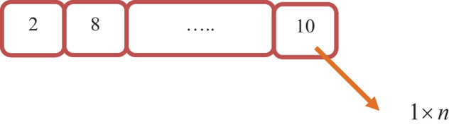
Encoding of Agent’s Location

This section describes the encoding location of agents, which is illustrated in Fig. 3. Solution encoding is utilized to pick the optimal CH according to the fitness function. Here, each part indicates the nodes’ index, and the solution dimension is $1\times n$, where $n$ depicts the number of required nodes. In addition, the selected CH does not surpass the total node count, and the selected path is from $2\to 8\to 10$.

Fig. 3.

Solution encoding

Fitness Function

The optimum solution is chosen using the fitness function. In this case, the fitness is calculated using variables including distance, energy, link quality, throughput, and delay.

$$\underset{min}{F_{\mathit{uv}}}=\frac{1}{h^2}\left[\sum _{u=1}^h\sum _{v=u+1}^h{G}_{\mathit{uv}}+g_{\mathit{uv}}+\left(1-Q_{\mathit{uv}}\right)+E(h_u)+(1-M_{\mathit{uv}})\right]$$ 8

where $G_{\mathit{uv}}$ specifies the distance, $g_{\mathit{uv}}$ indicates the delay, $Q_{\mathit{uv}}$ specifies the link quality, $M_{\mathit{uv}}$ indicates the throughput, and $E(h_u)$ specifies the consumed energy.

The fitness parameters are explained below.

1. Distance: It is the distance between the two specified nodes and is portrayed as

$$G_{\mathit{uv}}={\left|P_u-P_v\right|}_{\mathit{NF}}$$ 9

where $P_u-P_v$ indicates the distance among $u^{\mathit{th}}$ node and $v^{\mathit{th}}$ node and $\mathit{NF}$ specifies the normalization factor.

• b)Delay: The term delay is defined as the time taken to transfer data from source to destination. The formula is given as

$$g_{\mathit{uv}}=\frac{1}{P}\sum _{u=1}^n{h}_u$$ 10

where $P$ demonstrates the overall node count and $n$ specifies the node count in a path.

• iii)Link quality: It is expressed as the ratio between power consumed by the node $u$ and $v$, and the distance among the nodes $u$ and $v$, which is portrayed as,

$$Q_{\mathit{uv}}=\frac{X_{\mathit{uv}}}{G_{\mathit{uv}}}$$ 11

where $X_{\mathit{uv}}$ specifies the power consumed by the $u^{\mathit{th}}$ and $v^{\mathit{th}}$ node and $G_{\mathit{uv}}$ specifies the distance among the node $u$ and $v$.

• iv)Throughput: The term throughput is expressed as the successfully transmitted packets to the destination and is expressed in Eq. (13).

$$M_{\mathit{uv}}=\sum _{u=1}^h\frac{E_u\ast d_s}{D_p}$$ 12

where $E_u$ represents the energy of the node $u$, $d_s$ specifies the data packet size, and $D_p$ signifies the data packet.

• e)Energy consumption: Energy consumption, which is described in the “Energy Model” section, is used to calculate how much energy is used by each node.

Algorithmic Steps of EHBO+

• i)Initialization: The count of a honey badger with the population size as $Z$ and the respective locations are expressed as

$$f_d=L{B}_d+k_1\times \left(U{B}_d-L{B}_d\right)$$ 13

where $k_1$ designates the random number amid 0 and 1, $f_d$ denotes the placement of $d^{\mathit{th}}$ honey badger, and $U{B}_d$ and $L{B}_d$ denote the lower bound and upper bound.

• b)Intensity evaluation: The definition of intensity takes into account both the prey’s level of attention and their proximity to the honey badger. If any of the locations have a high smell, then the motion of prey is faster and is portrayed as

$$J_d=k_2\times \frac{W}{4\pi s_d^2}$$ 14

$$W={\left(f_d-f_{d+1}\right)}^2$$ 15

$$s_d=f_{\mathit{prey}}-f_d$$ 16

where $W$ signifies the strength of concentration and $s_d$ denotes the spacing between prey as well as $d^{\mathit{th}}$ badger.

• iii)Update the density factor: The density factor is renewed based on the time-changing randomization. Thus, the decreasing value of $\mathrm{\Xi }$ decreases the iteration count and is expressed as

$$\mathrm{\Xi }=K\times exp\left(\frac{-r}{r_{max}}\right)$$ 17

where $K$ specifies the constant, $\mathrm{\Xi }$ specifies the density factor, and $r_{\max }$ specifies the maximum iteration, which is greater than or equal to one.

• iv)Escape from local optimum: This process is done using two phases, namely, digging and honey phase. This algorithm utilizes the flag $D$, for altering the exploration direction to carefully study the search space.
• v)Renew the agent position: The location of the agent is updated based on two phases, like digging and honey phases.

Digging phase: The honey badger updates its location in a cardioid fashion throughout this phase, and its mobility is described as

$$f_{\mathit{new}}=f_{\mathit{prey}}+D\times \omega \times R\times f_{\mathit{prey}}+D\times k_3\times \mu \times s_d\times \left|\text{Cos}(2\pi k_4)\times \left(1-\text{Cos}(2\pi k_5\right)\right|$$ 18

where

$$s_d=f_{\mathit{prey}}(r)-f_d(r)$$ 19

Let us assume that

$$f_{\mathit{new}}=f_d(r+1)$$ 20

$$f_{\mathit{prey}}=f_{\mathit{prey}}(r)$$ 21

$$f_d=f_d(r)$$ 22

Substitute Eqs. (19), (20), (21), and (22) in Eq. (18), then the expression is

$$f_d(r+1)=f_{\mathit{prey}}(r)+D\times \omega \times R\times f_{\mathit{prey}}(r)+D\times k_3\times \mu \times \left|\text{Cos}(2\pi k_4)\times \left(1-\text{Cos}(2\pi k_5\right)\right|\times \left[f_{\mathit{prey}}(r)-f_d(r)\right]$$ 23

$$\begin{array}{c}{f}_d(r+1)=f_{\mathit{prey}}(r)+D\times \omega \times R\times f_{\mathit{prey}}(r)+D\times k_3\times \mu \times \left|\text{Cos}(2\pi k_4)\times \left(1-\text{Cos}(2\pi k_5\right)\right|\times f_{\mathit{prey}}(r)-\\ D\times k_3\times \mu \times \left|\text{Cos}(2\pi k_4)\times \left(1-\text{Cos}(2\pi k_5\right)\right|f_d(r)\\ \end{array}$$ 24

$$\begin{array}{c}{f}_d(r+1)=f_{\mathit{prey}}(r)\left[1+D\times \omega \times R+D\times k_3\times \mu \times \left|\text{Cos}(2\pi k_4)\times \left(1-\text{Cos}(2\pi k_5\right)\right|\right]-\\ D\times k_3\times \mu \times \left|\text{Cos}(2\pi k_4)\times \left(1-\text{Cos}(2\pi k_5\right)\right|f_d(r)\\ \end{array}$$ 25

From EWMA [25],

$$f_d^E(r)=\sigma f_d(r)+\left(1-\sigma \right)f_d^E(r-1)$$ 26

$$f_d(r)=\frac{1}{\sigma }\left[f_d^E(r)-\left(1-\sigma \right)f_d^E(r-1)\right]$$ 27

Applying Eq. (27) in Eq. (25), then the equation is

$$\begin{array}{c}{f}_d(r+1)=f_{\mathit{prey}}(r)\left[1+D\times \omega \times R+D\times k_3\times \mu \times \left|\text{Cos}(2\pi k_4)\times \left(1-\text{Cos}(2\pi k_5\right)\right|\right]-\\ D\times k_3\times \mu \times \left|\text{Cos}(2\pi k_4)\times \left(1-\text{Cos}(2\pi k_5\right)\right|\left[\frac{1}{\sigma }\left[f_d^E(r)-\left(1-\sigma \right)f_d^E(r-1)\right]\right]\\ \end{array}$$ 28

where $\omega \ge 1$, $k_4$, $k_4$, $k_5$, and $k_7$ denote the random number between 0 and 1, $f_d^E(r)$ shows the location of the honey badger using EWMA at $r^{\mathit{th}}$ iteration, $\omega \ge 1$ indicates the honey badger’s capability to catch the food, and $f_d^E(r-1)$ indicates the location of honey badger using EWMA at ${\left(r-1\right)}^{\mathit{th}}$ iteration.

$$D=\left\{\begin{array}{cc}1& if{k}_7\le 0.5\\ -1& \mathit{else}\end{array}\right)$$ 29

While performing the digging phase, the badger accepts the disturbance $D$, which permits the badger to evaluate the better location of prey.

Honey phase: Here, the honey badger obeys the rules of the honey bird for approaching the beehive, and this is articulated as

$$f_{\mathit{new}}=f_{\mathit{prey}}+D\times k_7\times \mu \times s_d$$ 30

where

$$s_d=f_{\mathit{prey}}-f_d$$ 31

Applying Eq. (31) in (30), then the expression can be portrayed as

$$f_{\mathit{new}}=f_{\mathit{prey}}+D\times k_7\times \mu \times \left(f_{\mathit{prey}}-f_d\right)$$ 32

$$f_{\mathit{new}}=f_{\mathit{prey}}\left(1+D\times k_7\times \mu \right)-D\times k_7\times \mu \times f_d$$ 33

Apply Eqs. (20), (21), and (22) on Eq. (33), then the expression is changed to

$$f_d(r+1)=f_{\mathit{prey}}(r)\left(1+D\times k_7\times \mu \right)-D\times k_7\times \mu \times f_d(r)$$ 34

Apply Eq. (27) in Eq. (34), then it is modified as

$$f_d(r+1)=f_{\mathit{prey}}(r)\left(1+D\times k_7\times \mu \right)-D\times k_7\times \mu \times \left[\frac{1}{\sigma }\left[f_d^E(r)-\left(1-\sigma \right)f_d^E(r-1)\right]\right]$$ 35

where

$$\mu =B\times exp\left(\frac{r}{r_{max}}\right)$$ 36

where $r_{max}$ specifies the highest iteration count, $B$ indicates the constant, which is greater than 1, $s_d$ indicates the distance between prey and $d^{\mathit{th}}$ honey badger, and $f_{\mathit{prey}}(r)$ denotes the location of prey.

• f)Evaluation of reliability: In this method, the best solution is acquired by Eq. (8), and the minimized value of the fitness function is portrayed as an optimal solution.
• g)Termination: The aforesaid processes are achieved repeatedly till the highest solution is achieved.

In this case, the established EHBO algorithm is used to transport information among the nodes via the most efficient route. Nodes are chosen in this case depending on the fitness function.

BC Detection at the BS

The BS runs the BC detection system, which is an EHBO-based DCNN. Here, ROI extraction is used for pre-processing, and feature extraction is used to isolate the important features, such as statistical features and texture features. The processes, such as rotation, flipping, cropping, and zooming are utilized to perform the data augmentation. After that, the BC classification is performed using DCNN, where the weights and bias are tuned with devised EHBO algorithm.

Let us assume the dataset $W$ with $d$ images, which are mathematically portrayed as

$$W=\left\{W_1,W_2,...,W_z,...,W_d\right\}$$ 37

where $W_z$ indicates the $z^{\mathit{th}}$ images and $d$ indicates the overall image count. $W_z$ is an input of RoI extraction.

Pre-processing

The pre-processed image speeds up the classifier’s classification performance while reducing computing time. ROI extraction refers to the process of extracting or filtering the specified region from images. It eliminates the noise that exists in the image. Moreover, the outcome of RoI extraction is represented as $X_R$, which is processed under segmentation.

Segmentation

The input of BC segmentation is $X_R$, and the segmentation is done with U-net. In this step, the segmented regions are separated from $X_R$. The advantage of the U-net model [27] is that it has less training time and the efficiency of segmentation is maximal. The structure of the U-net is designated in the next section.

U-net Structure

U-net architecture [27] is formed as in U-shape so that it is called as U-net model. The U-net architecture contains two paths, namely, contrasting path and expansive path. The contrasting path is placed on the left lobes, whereas the expansive path is placed on the right lobes. Here, the contrasting path comprises two conv layers, pooling layer, and ReLU with 2 strides for performing downsampling. In every step of downsampling, the feature channel counts are twined. In expansive path, each step comprises upsampling-dependent feature map with conv layers and ReLU layers, which reduces the feature channel to be halved. This method achieved the loss of border pixel, such that the process of cropping is performed at every convolution. Lastly, the conv layer is exploited to map all the feature vectors to the requisite class count. The BC segmented region gotten from the U-net model is characterized as $M_s$. Figure 4 depicts the design of the U-net model.

Fig. 4.

U-net architecture

Feature Extraction

The process of feature excavation is considered a technique for extracting the feature from a segmented image $M_s$. The dimension of the image is large; hence, it contains multiple numbers of features. Nonetheless, all the features do not have huge information about the image. Thus, only the texture features with huge information about the image is extracted in this step.

Texture feature extraction: The texture features, such as LGBP, GLCM, and LOOP, are excavated from the pre-processed image. After extracting the texture features, the extracted features are processed under data augmentation for augmenting the accuracy of classification. Then, the statistical features are excerpted from the augmented image. The mathematical expansion of LGBP, GLCM, and LOOP features are explained below.

LGBP: LGBP operator [20] is attained by encoding the magnitude values of the LBP operator. Let us assume the center value as $h_m$ and the neighboring pixel as $h_p$, then the computation of the LGBP operator is expressed as

$$\Re \left(h_p-h_m\right)=\left\{\begin{array}{c}\begin{array}{cc}1,& h_p\ge h_m\end{array}\\ \begin{array}{cc}0,& h_p<h_m\end{array}\end{array}\right)$$ 38

Moreover, the LBP pattern of the pixel value is computed by assigning the binomial factor ${}^p$ for every $\Re \left(h_p-h_m\right)$ and is expressed as

$$LBP=\sum _{p=0}^7\Re \left(h_p-h_m\right)2^p$$ 39

Equation (39) signifies the spatial pattern of local image texture. Moreover, the LGBP feature is indicated as $n_1$.

GLCM feature: GLCM [21] is a statistical method that analyzes the texture feature from an image based on the spatial relationship among pixels. GLCM is in the form of a matrix where the rows and columns of the matrix are similar to the gray level count. In this paper, numerous features are excerpted from GLCM, which is mathematically indicated as$a_u(l)=\sum _{t=0}^{C-1}A\left(l,t\right)$ and 

$$a_v(t)=\sum _{l=0}^{C-1}A\left(l,t\right)$$ 40

${\alpha }_u=\sum _{l=0}^{G-1}l{A}_u(l)$ and

$${\alpha }_v=\sum _{t=0}^{G-1}t{a}_v(t)$$ 41

$${\beta }_u^2=\sum _{l=0}^{G-1}{\left(A_u(l)-{\alpha }_u(l)\right)}^2$$ 42

$${\beta }_v^2=\sum _{t=0}^{G-1}{\left(A_v(t)-{\alpha }_v(t)\right)}^2$$ 43

where $C$ depicts the gray level count, $\alpha$ signifies the mean value of $A$, ${\alpha }_u$, ${\alpha }_v$, ${\beta }_u$, and ${\beta }_v$ demonstrates the mean and standard deviation of $A_u$ and $A_v$. Thus, the GLCM feature is represented as $n_2$.

LOOP features: The rotation invariance is encoded into the leading formulation by the LOOP descriptor [22]. The LOOP algorithm also bargains the empirical conveyance of extraneous parameters. Thus, the LOOP value of the pixel $\left(u_d,v_d\right)$ is portrayed as

$$LOOP\left(u_d,v_d\right)=\sum _{p=1}^{7}Z(e_p-e_m).2^{r_p}$$ 44

$$Z(u)=\left\{\begin{array}{cc}1& ifu\ge 0\\ 0& \mathit{Otherwise}\end{array}\right)$$ 45

where $e_p$ and $e_m$ are the pixel intensities and $Z(u)$ be the Kirsch function. The LOOP feature is represented as $n_3$. Thus, the final texture-based feature vector is formed by joining all the texture features, which is formulated as

$$N=\left\{n_1,n_2,n_3\right\}$$ 46

where $n_1$ specifies the LGBP feature, $n_2$ specifies the GLCM feature, and $n_3$ denotes the LOOP feature. In this step, the texture features are only extracted. Then, the segmented image is then expanded using data augmentation. Therefore, the texture features are extracted before augmentation. Further, the statistical features are extracted after the data augmentation.

Data Augmentation

Before classifying the BC, data augmentation [28] is necessary to improve the classification. The extracted texture features, such as $n_1$, $n_2$, and $n_3$ are presented to the data augmentation. Here, the processes, such as rotation, flipping, cropping, and zooming are performed separately on each feature, thereby a total of 12 images are attained in the data augmentation process. Moreover, a brief description of the data augmentation process is given below.

Rotation: This step shifts the image to a specified degree around the center with mapping of each pixel of an image.

Flipping: The process of flipping is performed across the vertical axis, which is computationally effective and easy to execute.

Cropping: This step crops or extracts the significant features from the corner or center of an image.

Zooming: This process is used to zoom-in or zoom-out the processed image.

Thus, the data-augmented outcome is portrayed as $D_A$.

Statistical feature extraction: The statistical features [29], like area, energy, homogeneity, mean, variance, entropy, kurtosis, skewness, and HOG, are extracted from the augmented outcome $D_A$. Here, the statistical features are computed for every augmented image. Moreover, the expression for statistical features is portrayed as

• i)Area: Area is one of the significant statistical features, which is expressed as the number of pixels in a boundary surrounded by the affected area in the segmented image quantified as area. Thus, the notation for the area is $y_1$ with dimension $1\times 1$.
• ii)Energy: Based on energy, also known as the angular second moment, the mathematical form of energy is calculated and is written as

$$Energy=\sum _{u,v=0}^{}A{(u,v)}^2$$ 47

where $A(u,v)$ depicts the area of the pixel location. Thus, the energy output is denoted as $y_2$ with size $1\times 1$.

• iii)Homogeneity: Homogeneity refers to the local information, which portrays the regularity of computed area and is expressed as

$$Homogeneity=\sum _{u,v=0}^{}\frac{A(u,v)}{1+\left|u-v\right|}$$ 48

Thus, the homogeneity outcome is $y_3$ with dimension $1\times 1$.

• iv)Mean: The term mean refers to the average intensity values of every pixel and is demonstrated as

$$Mean=\frac{{\sum }_{u=1}^n{V}_u}{n}$$ 49

where $V_u$ indicates the sum of all pixel values. Moreover, the output for the mean is $y_4$ with dimension $1\times 1$.

• xxii)Variance: The term variance refers to the dissimilarities of intensities among the pixels and is indicated as

$$Variance=\frac{{\sum }_{u=0}^{N-1}{\left(\alpha (u)-{\alpha }^2\right)}^2}{N}$$ 50

Here, the term $y_5$ is the output of variance with dimension $1\times 1$.

• f)Entropy: The term entropy is used to express the texture of an image, and the expression becomes

$$Entropy=-\sum _{u=0}^{N-1}\sum _{v=0}^{N-1}A(u,v){log}_{2}A(u)$$ 51

The entropy output is denoted as $y_6$ with dimension $1\times 1$.

• vii)Kurtosis: It characterizes the data distribution of the peak of the signal created as compared with normal distribution and is indicated as

$$Kurtosis=\frac{{\kappa }_4}{{\varsigma }^4}$$ 52

where ${\kappa }_4$ depicts the fourth moment of mean, $\varsigma$ indicates the standard deviation. Here, the kurtosis is indicated as $y_7$ with dimension is $1\times 1$.

• viii)Skewness: Skewness is utilized to compute the abnormality of information around the average of the sample and is illustrated as

$$skewness=\frac{{\sum }_{u=1}^n\left(V_u-\overline{V}\right)}{{\left(n-1\right)}^3}$$ 53

where the skewness is indicated as $y_8$ with dimension $1\times 1$.

• i)HOG: HOG feature is a descriptor, which is calculated by partitioning the region of the frame into cells. For every cell, a local 1D histogram of the gradient is applied on every pixel of a cell. The HOG feature is represented as $y_9$.

Thus, the final vector is generated by joining all the statistical features and is expressed as

$$F=\left\{y_1,......,y_9\right\}$$ 54

where $y_1$ denotes the area feature, $y_2$ signifies the energy, $y_3$ denotes the homogeneity, $y_4$ signifies the mean, $y_5$ portrays the variance, $y_6$ specifies the entropy, $y_7$ denotes the kurtosis, $y_8$ indicates the skewness, and $y_9$ specifies the HOG. Following the generation of statistical characteristics, Deep CNN was trained using a hybrid optimization algorithm to classify BC.

BC Classification

The extracted feature $F$ is fed to the input of Deep CNN to categorize the image into either normal or abnormal. Deep CNN [24] is a DL classifier, which is widely utilized for classification purposes. This method has multiple conv layers, which enhances the prediction accuracy.

Structure of Deep CNN

Deep CNN [24] contains three layers, such as convolutional layer, FC layer, and pooling layer; each of these layers performs a separate operation. The conv layer performs the feature extraction process, pool layer performs the sub-sampling process, and the FC layer performs the classification process. Deep CNN contains numerous quantity of conv layers, which progresses the detection efficiency. The structure of Deep CNN is portrayed in Fig. 5 in which its input vector is indicated as $F$.

Fig. 5.

Structure of Deep CNN

Conv layer: The conv layer contains the multiple counts of succeeding layers and is the most important layer in Deep CNN. Additionally, the conv layer count affects how accurately predictions are made. Utilizing accessible fields, the conv layers’ neurons are coupled to the trainable weights.

$${\left(C_b^q\right)}_{w,z}={\left(x_b^q\right)}_{w,z}+\sum _{o=1}^{g_1^{b-1}}\sum _{i=-j_1^b}^{j_1^b}\sum _{c=-j_2^b}^{j_2^b}{\left(r_{q,o}^b\right)}_{i,c}\ast {\left(C_b^{q-1}\right)}_{w+i,z+c}$$ 55

where ${\left(C_b^q\right)}_{w,z}$ characterizes the feature map of $b^{\mathit{th}}$ conv layers, $x_b^q$ shows the bias at $b^{\mathit{th}}$ conv layers, and ${\left(r_{q,o}^b\right)}_{i,c}$ and ${\left(C_b^{q-1}\right)}_{w+i,z+c}$ describe the kernel function in $b^{\mathit{th}}$ conv layers.

ReLU layer: ReLU is considered as an activation function, which is used to eliminate the negative values to progress the effectiveness. Moreover, the outcome of the ReLU layer is portrayed as

$$C_b^q=fun(C_z^{q-1})$$ 56

where $fun()$ indicates the activation function of the conv layer $b$.

Pooling layers: Pooling layers perform the sub-sampling process by minimizing the feature maps for improving the invariance features to the input data distortions. In this layer, there is no bias or weight as it is a non-parameterized layer.

FC layer: The FC layer is used to perform the classification or prediction process. In this paper, the FC layer is used to classify the BC disease, and this layer is portrayed as

$$T_b^q=\rho \left(L_b^q\right)with{L}_b^q=\sum _{o=1}^{g_1^{b-1}}\sum _{i=-j_1^b}^{j_1^b}\sum _{c=-j_2^b}^{j_2^b}{\left(r_{q,o}^b\right)}_{i,c}\ast {\left(C_b^{q-1}\right)}_{w+i,z+c}$$ 57

Hence, the output attained by DCNN is articulated as $S_x^{\ast }$.

Training of Deep CNN Using EHBO Algorithm

This sector denotes the Deep CNN training procedure employing the created EHBO algorithm. In addition, the fitness function of the EHBO for training the Deep CNN is MSE, which is portrayed as

$$Fitness=\frac{1}{c}\sum _{x=1}^c{\left[S_x-S_x^{\ast }\right]}^2$$ 58

where $c$ indicates the overall sample count, $S_x$ indicates the expected outcome, and $S_x^{\ast }$ specifies the predicted result of Deep CNN.

Results and Discussion

This section describes the outcomes and a discussion of the new EHBO algorithm for BC classification.

Experimental Setup

The testing of devised EHBO algorithm is carried out on MATLAB tool, intel i3 core processor with Windows 10 OS. Table 1 displays the experimental setup of the implemented system.

Table 1.

Experimental setup

Parameters	Values
Epoch	20
Batch size	32
Learning rate	0.001
Optimization iteration	100
Upper bound	30
Lower bound	0

Dataset Description

The newly devised EHBO algorithm is implemented using the MIAS and the DDSM dataset [28].

MIAS dataset: This dataset comprises 322 digitized films, which persist on 2.3 GB 8-mm tape. It also contains the “truth” of the radiologist and the location of any irregularities that persist in the image.

DDSM dataset: DDSM is another resource of mammographic images for the research community. Here, the dataset contains two images of both breasts and their correlated patient information. Moreover, the images comprise affected areas with information about localities and types of suspicious areas.

Evaluation Metrics

The evaluation metrics are described as follows:

• i)  Testing accuracy: The testing accuracy is expressed as the ratio of the number of appropriately classified samples to the overall tested samples. The testing accuracy formula is depicted below:

$$\mathrm{A}=\frac{H^p+I^n}{H^p+H^n+I^p+I^n}$$ 59

where $H^p$ shows the true positive, $H^n$ denotes the true negative, $I^p$ represents false positive, and $I^n$ means false negative.

• b)Sensitivity: The sensitivity is defined as the probability of producing a positive result and is expressed as

$$\mathrm{E}=\frac{H^p}{H^p+I^n}$$ 60

• iii)Specificity: Specificity is defined as the probability of producing a negative result and is illustrated as

$$\mathrm{K}=\frac{H^n}{H^n+I^p}$$ 61

Observational Outcome

The observational outcome of the EHBO algorithm is specified in Fig. 6. Here, the input image is given in Fig. 6a, the segmented image is specified in Fig. 6b, the outcome of the HOG feature is portrayed in Fig. 6c, the extracted LGBP is explained in Fig. 6d, the extracted LOOP features are given in Fig. 6e, the output image of flipped features are given in Fig. 6f, the outcome of rotated image is given in Fig. 6g, the outcome of zoomed image is given in Fig. 6h, and the outcome of cropped image is given in Fig. 6i.

Fig. 6.

Experimental outcome. a Input image, b segmented image, c HOG feature, d LGBP feature, e LOOP feature, f flipped image, g rotated image, h zoomed image, and i cropped image

The screenshots of the experiment performed is specified in Fig. 7.

Fig. 7.

Screenshot of the experiment performed

Comparative Methods

The effectiveness of the devised algorithm is analyzed with other alternative CN classification algorithms, such as MLP classifier [13], deep learning [8], SVM [16], and ensemble-based classifier [6].

For routing, the various algorithms, such as MACO_QCR protocol [30], hierarchical cluster-based routing protocol [31], energy efficient routing protocol [32], and chain cluster-based routing [33] are utilized to compare the routing performance with EHBO-based routing.

The description of comparative methods is depicted in Table 2.

Table 2.

Description of comparative methods

Method	Description
Classification methods
Multi-layer perceptron (MLP) classifier [13]	In this research, the BC is identified in its early stage, and the prediction performance was improved using MLP classifier, by reducing the Relative Absolute Error rate.
Deep learning [8]	The CNN-based deep model was used for BC detection using histopathology images. Here, the graphics processing unit was used to train the deep learning model to attain better outcomes.
Support vector machine (SVM) [16]	Here, the best features were selected using recursive feature selection, and based on that, the classification was done by SVM.
Ensemble-based classifier [6]	In this approach, the malignant cells were detected based on extracting textured-based features and shapes, and the classification was done by the ensemble-based classifier.
Routing methods
Multi-objective ant-colony-optimization-based QoS-aware cross-layer routing (MACO_QCR) protocol [30]	This protocol was proposed to do the communication in WSN. Here, the fuzzy membership function was used as the fitness function.
Hierarchical cluster-based routing protocol [31]	In this approach, the hierarchical cluster-based routing protocol was proposed for reducing the consumption of energy and increasing the lifetime of the network. Here, the optimal solution was identified using the convex function.
Energy efficient routing protocol [32]	In this research, an energy-efficient protocol, named, ring routing was developed for reducing the overhead in WSN.
Chain cluster-based routing [33]	This method had the advantages of both LEACH and PEGASIS. It reduced the energy consumption and network delay.

Comparative Assessment

The comparative evaluation of devised EHBO-based DCNN is analyzed by modifying the training data % utilizing MIAS and DDSM datasets.

Comparative Assessment Using DDSM

The achieved values of sensitivity, accuracy, and specificity according to the devised scheme are given in Fig. 8. Figure 8a shows the accuracy analysis. Here, the accuracy of 0.9051 is attained by the devised scheme, whereas the accuracy of 0.8396, 0.8451, 0.8563, and 0.8738 is gotten by the other conventional BC classification techniques, like MLP classifier, deep learning, SVM, and ensemble-based classifier for the training data is 90%. Moreover, the improved percentages of projected approach with conventional techniques are 7.23%, 6.62%, 5.39%, and 3.45%. Figure 8b demonstrates the sensitivity of the projected BC classification technique by altering the training data from 50 to 90%. When the training data is maximum, then the sensitivity is 0.8971 for the new EHBO-based DCNN, and the sensitivity is 0.8268 for the MLP classifier, 0.8303 for deep learning, 0.8415 for SVM, and 0.8797 for the ensemble-based classifier. In addition, the devised EHBO algorithm acquired improved performance with the conventional scheme in terms of percentages 7.83%, 7.44%, 6.19%, and 1.93%. The specificity analysis is given in Fig. 8c. The specificity of EHBO-based DCNN is 0.9029, MLP classifier is 0.822, deep learning is 0.8417, SVM is 0.8526, and ensemble classifier is 0.8669, while 90% of training data is processed. The performance improvement of EHBO-based DCNN is 8.96%, 6.77%, 5.57%, and 3.98%. Figure 8d demonstrates the ROC analysis of EHBO-based BC classification. If the FPR value is 90, then the TPR of EHBO-based BC classification is 0.9365, whereas the conventional approaches are 0.8975, 0.8803, 0.8990, and 0.8616.

Fig. 8.

Comparative analysis of EHBO-based DCNN in terms of a testing accuracy, b sensitivity, c specificity, and d ROC analysis

The observational outcome of the projected scheme based on energy and distance is demonstrated in Fig. 9. The energy values of the developed technique using the DDSM dataset are shown in Fig. 9a. The MACO QCR protocol, the hierarchical cluster-based routing protocol, the energy efficient routing protocol, and the chain cluster-based routing all acquired energy values of 0.101 J, 0.097 J, 0.102 J, and 0.107 J, respectively, when the round is 501, while the newly developed EHBO-based routing is 0.112. Figure 9b demonstrates the distance value measured by the various BC classification techniques. When the number of rounds is 401, then the existing and devised BC classification technique measured the distance of 39.30 km, 36.65 km, 38.02 km, 42.04 km, and 31.65 km, respectively.

Fig. 9.

Comparative assessment based on a energy and b distance

Comparative Assessment Using MIAS

The measured values of sensitivity, accuracy, and specificity according to the devised scheme are given in Fig. 10. Figure 10a illustrates the testing accuracy of the projected BC classification technique by adjusting the training data from 50 to 90%. When the training data is 90%, then the testing accuracy is 0.9015 for the EHBO-based DCNN and the testing accuracy is 0.8271 for the MLP classifier, 0.8326 for deep learning, 0.8525 for SVM, and 0.8813 for the ensemble-based classifier. In addition, the devised EHBO algorithm acquired improved performance with the conventional scheme in terms of percentages 8.25%, 7.64%, 5.43%, and 2.24%. Figure 10b shows the EHBO-based DCNN’s sensitivity. While 90% of the training data is processed, the sensitivity of the EHBO-based DCNN is 0.9058, the MLP classifier is 0.8314, deep learning is 0.8369, SVM is 0.8568, and ensemble classifier is 0.8856. In addition, the improved percentage of EHBO-based DCNN is 8.21%, 7.60%, 5.40%, and 2.23%. Figure 10c shows the specificity analysis. Here, for the training data is 90%, the specificity attained by the devised scheme is 0.9029, whereas the specificity is 0.822, 0.8417, 0.8526, and 0.8669 for the techniques, like MLP classifier, deep learning, SVM, and ensemble-based classifier. Figure 10d demonstrates the ROC analysis. For 90% FPR, the TPR of EHBO-based BC classification is 0.9532, whereas the MLP classifier, deep learning, SVM, and ensemble-based classifier have the TPR of 0.9084, 0.8803, 0.8990, and 0.8634, respectively.

Fig. 10.

Comparative analysis of EHBO-based DCNN in terms of a testing accuracy, b sensitivity, c specificity, and d ROC analysis

The outcome of the projected scheme based on energy and distance is shown in Fig. 11. Figure 11a portrays the energy values attained by the devised scheme. For round 501, then the existing routing methods acquired the energy values of 0.101 J, 0.097 J, 0.102 J, and 0.107 J, whereas the projected EHBO-based routing attained the energy of 0.111 J. Figure 11b provides the distance value recorded by the several BC classification approaches. As the round is 401, then the existing and devised BC classification technique achieved the distance of 38.94 km, 36.89 km, 33.70 km, 36.92 km, and 31.36 km, correspondingly.

Fig. 11.

Comparative assessment based on a energy and b distance

Comparative Discussion

Table 3 displays a comparison of the developed EHBO-based DCNN method for classifying BC. In this study, two datasets, the DDSM and MIAS datasets, are used to classify BC. From Table 2, the projected EHBO-based DCNN attained a better performance correlating to the DDSM dataset. The recorded values of testing accuracy, sensitivity, and specificity according to the devised EHBO-based DCNN are 0.9051, 0.8971, and 0.9029, correspondingly. Similarly, the test accuracy of the MLP classifier, deep learning, SVM, and ensemble-based classifier is 0.8396, 0.8451, 0.8563, and 0.8738, sensitivity of 0.8268, 0.8303, 0.8415, and 0.8797, and the specificity is 0.822, 0.8417, 0.8526, and 0.8669, correspondingly.

Table 3.

Comparative discussion

Database	DDSM			MIAS
	Testing accuracy	Sensitivity	Specificity	Testing accuracy	Sensitivity	Specificity
MLP classifier	0.8396	0.8268	0.822	0.8271	0.8314	0.8327
Deep learning	0.8451	0.8303	0.8417	0.8326	0.8369	0.8382
SVM	0.8563	0.8415	0.8526	0.8525	0.8568	0.8581
Ensemble-based classifier	0.8738	0.8797	0.8669	0.8813	0.8856	0.8869
Proposed EHBO-based DCNN	0.9051	0.8971	0.9029	0.9015	0.9058	0.9071

Due to the extraction of useful features, the developed approach performed better in this study than the traditional techniques. Generally, the segmented region contains excess features, but all those features are not significant. Thus, the developed technique extracts only the significant features, such as area, energy, homogeneity, mean, variance, entropy, kurtosis, skewness, and HOG, and the texture features, which improves the efficacy of predicted outcomes in terms of evaluation metrics.

Conclusion

This paper presents the new EHBO-based DL algorithm for BC classification using MIAS and DDSM datasets. The devised method attained improved classification accuracy and high processing speed, due to the integral use of effective segmentation and feature extraction. The tumor region from the processed image is isolated by the U-net model. From the segmented region, the significant features, like area, energy, homogeneity, mean, variance, entropy, kurtosis, skewness, and HOG, and the texture features have been extracted. Moreover, the devised scheme gathers the record of every referred patient to attain better classification accuracy. The gathered information is transmitted to the BS using devised EHBO algorithm for classifying the BC, and the classification process is done with DCNN. Here, the EHBO is a combination of the EWMA and HBO algorithms, which perform two functions, such as routing and tuning the weights of DCNN. The observational outcome reveals that the projected EHBO-based DCNN algorithm attained outstanding performance based on the test accuracy, sensitivity, and specificity of 0.9051, 0.8971, and 0.9029, correspondingly. To further improve the BC diagnosis system’s performance, deep learning classification methods, optimization, and other characteristic selection algorithms will be applied in the future.

Nomenclature

BC

Breast cancer

EHBO

Exponential Honey Badger Optimization

DCNN

Deep Covolutional Neural Network

IoT

Internet of Things

HBO

Honey Badger Optimization

EWMA

Exponential Weighted Moving Average

BS

Base station

HOG

Histogram of oriented gradients

LGBP

Local Gabor Binary Pattern

GLCM

Gray-Level Co-occurrence Matrix

LOOP

Local Optimal Oriented Pattern

MLP

Multi-layer perceptron

DL

Deep learning

SVM

Support vector machine

WDBC

Wisconsin Diagnostic BC

WPBCC

Wisconsin Prognostic BC Chemotherapy

ML

Machine learning

OKM-ANFIS

Optimized K-means-based adaptive neuro-fuzzy inference system

CH

Cluster head

conv

Convolutional

ReLU

Rectified linear unit

FC

Fully connected

MIAS

Mammographic Image Analysis Society

CNN

Convolutional Neural Network

DDSM

Digital Database for Screening Mammography

IMS

Intelligent Monitoring System

MACO_QCR

Multi-objective ant-colony-optimization based QoS-aware cross-layer routing

PEGASIS

Power efficient gathering in sensor information systems

WSN

Wireless Sensor Network

LEACH

Low-energy adaptive clustering hierarchy

Author Contributions

All authors have made substantial contributions to conception and design, revising the manuscript, and the final approval of the version to be published.

Data Availability

The data underlying this article are available in MIAS and DDSM datasets, at https://www.mammoimage.org/databases/.

Declarations

Ethical Approval

Not applicable.

Informed Consent

Not applicable.

Conflict of Interest

The authors declare no competing interests.

Disclaimer

Also, all authors agreed to be accountable for all aspects of the work in ensuring that questions related to the accuracy or integrity of any part of the work are appropriately investigated and resolved.

References

- 1.Al-Turjman F, Alturjman S. Context-sensitive access in industrial internet of things (IIoT) healthcare applications. IEEE Transactions on Industrial Informatics. 2018;14(6):2736–2744. doi: 10.1109/TII.2018.2808190. [DOI] [Google Scholar]
- 2.Deebak BD, Al-Turjman F, Aloqaily M, Alfandi O. An authentic-based privacy preservation protocol for smart e-healthcare systems in IoT. IEEE Access. 2019;7:135632–135649. doi: 10.1109/ACCESS.2019.2941575. [DOI] [Google Scholar]
- 3.Al-Turjman F, Zahmatkesh H, Mostarda L. Quantifying uncertainty in internet of medical things and big-data services using intelligence and deep learning. IEEE Access. 2019;7:115749–115759. doi: 10.1109/ACCESS.2019.2931637. [DOI] [Google Scholar]
- 4.Manogaran G, Lopez D, Chilamkurti N. In-Mapper combiner based MapReduce algorithm for processing of big climate data. Future Generation Computer Systems. 2018;86:433–445. doi: 10.1016/j.future.2018.02.048. [DOI] [Google Scholar]
- 5.Kharya S, Soni S. Weighted naive bayes classifier: a predictive model for breast cancer detection. International Journal of Computer Applications. 2016;133(9):32–37. doi: 10.5120/ijca2016908023. [DOI] [Google Scholar]
- 6.Khan SU, Islam N, Jan Z, Din IU, Khan A, Faheem Y. An e-Health care services framework for the detection and classification of breast cancer in breast cytology images as an IoMT application. Future Generation Computer Systems. 2019;98:286–296. doi: 10.1016/j.future.2019.01.033. [DOI] [Google Scholar]
- 7.Anand P, Kunnumakara AB, Sundaram C, Harikumar KB, Tharakan ST, Lai OS, Sung B, Aggarwal BB. Cancer is a preventable disease that requires major lifestyle changes. Pharmaceutical research. 2008;25(9):2097–2116. doi: 10.1007/s11095-008-9661-9. [DOI] [PMC free article] [PubMed] [Google Scholar]
- 8.Zahir S, Amir A, Zahri NAH, Ang WC. Applying the deep learning model on an IoT board for breast cancer detection based on histopathological images. In Journal of Physics: Conference Series. 2021;1755(1):012026. [Google Scholar]
- 9.Khamparia A, Bharati S, Podder P, Gupta D, Khanna A, Phung TK, Thanh DN. Diagnosis of breast cancer based on modern mammography using hybrid transfer learning. Multidimensional systems and signal processing. 2021;32(2):747–765. doi: 10.1007/s11045-020-00756-7. [DOI] [PMC free article] [PubMed] [Google Scholar]
- 10.Barracliffe, L., Arandjelovic, O. and Humphris, G., “A pilot study of breast cancer patients: can machine learning predict healthcare professionals’ responses to patient emotions”, In Proceedings of the International Conference on Bioinformatics and Computational Biology, Honolulu, HI, USA, pp. 20-22, 2017.
- 11.Alzubi JA, Manikandan R, Alzubi OA, Qiqieh I, Rahim R, Gupta D, Khanna A. Hashed Needham Schroeder industrial IoT based cost optimized deep secured data transmission in cloud. Measurement. 2019;150:107077. doi: 10.1016/j.measurement.2019.107077. [DOI] [Google Scholar]
- 12.Sharma, A., Kulshrestha, S. and Daniel, S., “Machine learning approaches for breast cancer diagnosis and prognosis”, In 2017 International Conference on Soft Computing and Its Engineering Applications (icSoftComp), pp. 1-5, 2017.
- 13.Gopal VN, Al-Turjman F, Kumar R, Anand L, Rajesh M. Feature selection and classification in breast cancer prediction using IoT and machine learning. Measurement. 2021;178:109442. doi: 10.1016/j.measurement.2021.109442. [DOI] [Google Scholar]
- 14.Savitha V, Karthikeyan N, Karthik S, Sabitha R. A distributed key authentication and OKM-ANFIS scheme based breast cancer prediction system in the IoT environment. Journal of Ambient Intelligence and Humanized Computing. 2021;12(2):1757–1769. doi: 10.1007/s12652-020-02249-8. [DOI] [Google Scholar]
- 15.Chokka, A. and Rani, K.S., “AdaBoost with feature selection using IoT to bring the paths for somatic mutations evaluation in cancer”, In Internet of Things and Personalized Healthcare Systems, pp. 51-63, 2019.
- 16.Memon, M.H., Li, J.P., Haq, A.U., Memon, M.H. and Zhou, W., “Breast cancer detection in the IOT health environment using modified recursive feature selection”, wireless communications and mobile computing, 2019.
- 17.Suresh A, Udendhran R, Balamurgan M, Varatharajan R. A novel internet of things framework integrated with real time monitoring for intelligent healthcare environment. Journal of medical systems. 2019;43(6):1–10. doi: 10.1007/s10916-019-1302-9. [DOI] [PubMed] [Google Scholar]
- 18.Nguyen, T.D., Khan, J.Y. and Ngo, D.T., “An effective energy-harvesting-aware routing algorithm for WSN-based IoT applications”, In proceedings of 2017 IEEE International Conference on Communications (ICC), pp. 1-6, 2017.
- 19.Yadav AK, Tripathi S. QMRPRNS: design of QoS multicast routing protocol using reliable node selection scheme for MANETs. Peer-to-Peer Networking and Applications. 2017;10(4):897–909. doi: 10.1007/s12083-016-0441-8. [DOI] [Google Scholar]
- 20.Zhang, W., Shan, S., Gao, W., Chen, X. and Zhang, H., “Local gabor binary pattern histogram sequence (lgbphs): a novel non-statistical model for face representation and recognition”, In Tenth IEEE International Conference on Computer Vision (ICCV'05) Volume 1, Vol. 1, pp. 786-791, 2005.
- 21.Zulpe N, Pawar V. GLCM textural features for brain tumor classification. International Journal of Computer Science Issues (IJCSI) 2012;9(3):354. [Google Scholar]
- 22.Chakraborti, T., McCane, B., Mills, S. and Pal, U., “LOOP descriptor: encoding repeated local patterns for fine-grained visual identification of Lepidoptera”, Computer Vision and Pattern Recognition, 2017.
- 23.Lakshmi, N.D., Latha, Y.M. and Damodaram, A., “Silhouette extraction of a human body based on fusion of HOG and graph-cut segmentation in dynamic backgrounds”, 2013.
- 24.Sugave S, Jagdale B. Monarch-EWA: Monarch-earthworm-based secure routing protocol in IoT. The Computer Journal. 2020;63(6):817–831. doi: 10.1093/comjnl/bxz135. [DOI] [Google Scholar]
- 25.Saccucci MS, Amin RW, Lucas JM. Exponentially weighted moving average control schemes with variable sampling intervals. Communications in Statistics-simulation and Computation. 1992;21(3):627–657. doi: 10.1080/03610919208813040. [DOI] [Google Scholar]
- 26.Hashim FA, Houssein EH, Hussain K, Mabrouk MS, Al-Atabany W. Honey Badger Algorithm: new metaheuristic algorithm for solving optimization problems. Mathematics and Computers in Simulation. 2022;192:84–110. doi: 10.1016/j.matcom.2021.08.013. [DOI] [Google Scholar]
- 27.Ronneberger, O., Fischer, P. and Brox, T., “U-net: convolutional networks for biomedical image segmentation”, In Proceedings of International Conference on Medical Image Computing and Computer-Assisted Intervention, pp. 234-241, 2015.
- 28.MIAS and DDSM dataset will be gathered from, https://www.mammoimage.org/databases/, accessed on January 2022.
- 29.L. Malliga, “A novel statistical based methodology for the feature extraction of both MRI and CT images”, International Journal of Engineering and Advanced Technology (IJEAT), Volume-8, Issue-6S3, 2019.
- 30.Kaur T, Kumar D. MACO-QCR: multi-objective ACO-based QoS-aware cross-layer routing protocols in WSN. IEEE Sensors Journal. 2020;21(5):6775–6783. doi: 10.1109/JSEN.2020.3038241. [DOI] [Google Scholar]
- 31.Ke W, Yangrui O, Hong J, Heli Z, Xi L. Energy aware hierarchical cluster-based routing protocol for WSNs. The Journal of China Universities of Posts and Telecommunications. 2016;23(4):46–52. doi: 10.1016/S1005-8885(16)60044-4. [DOI] [Google Scholar]
- 32.Tunca C, Isik S, Donmez MY, Ersoy C. Ring routing: an energy-efficient routing protocol for wireless sensor networks with a mobile sink. IEEE Transactions on Mobile Computing. 2014;14(9):1947–1960. doi: 10.1109/TMC.2014.2366776. [DOI] [Google Scholar]
- 33.Tang, F., You, I., Guo, S., Guo, M. and Ma, Y., “A chain-cluster based routing algorithm for wireless sensor networks”, journal of intelligent manufacturing, vol.23, no.4, pp.1305-1313, 2012.
Associated Data
This section collects any data citations, data availability statements, or supplementary materials included in this article.
Data Availability Statement