Deep neural networks with controlled variable selection for the identification of putative causal genetic variants

Abstract

Deep neural networks (DNNs) have been successfully utilized in many scientific problems for their high prediction accuracy, but their application to genetic studies remains challenging due to their poor interpretability. Here we consider the problem of scalable, robust variable selection in DNNs for the identification of putative causal genetic variants in genome sequencing studies. We identified a pronounced randomness in feature selection in DNNs due to its stochastic nature, which may hinder interpretability and give rise to misleading results. We propose an interpretable neural network model, stabilized using ensembling, with controlled variable selection for genetic studies. The merit of the proposed method includes: flexible modelling of the nonlinear effect of genetic variants to improve statistical power; multiple knockoffs in the input layer to rigorously control the false discovery rate; hierarchical layers to substantially reduce the number of weight parameters and activations, and improve computational efficiency; and stabilized feature selection to reduce the randomness in identified signals. We evaluate the proposed method in extensive simulation studies and apply it to the analysis of Alzheimer’s disease genetics. We show that the proposed method, when compared with conventional linear and nonlinear methods, can lead to substantially more discoveries.

Recent advances in whole genome sequencing (WGS) technology have led the way in exploring the contribution of common and rare variants in both coding and non-coding regions towards risk for complex traits. One main theme in WGS studies is to understand the genetic architecture of disease phenotypes and, crucially, provide a credible set of well-defined, novel targets for the development of genomic-driven medicine¹. However, the identification of causal variants in these datasets remains challenging due to the sheer number of genetic variants, the low signal-to-noise ratio and strong correlations among genetic variants. Most of the results published so far are derived from marginal association models that regress an outcome of interest on the linear effect of a single or multiple genetic variants in a gene^2,3. The marginal association tests are well-known for their simplicity and effectiveness, but they often identify proxy variants that are only correlated with the true causal variants and may fail to capture nonlinear effects, including but not limited to non-additive and interaction (epistatic) effects, which are thought to represent a substantial component of the missing heritability associated with current genome-wide association studies (GWAS)⁴. Recent studies on Alzheimer’s Disease (AD) genetics have identified genes whose effects are modulated by the APOE genotype (interaction effects), for example, GPAA1, ISYNA1, OR8G5, IGHV3–7 and SLC24A3^5–9. Moreover, Costanzo et al.¹⁰ and Kuzmin et al.¹¹ took a systematic approach to map genetics interactions among gene pairs and high-order interactions. The results highlighted the potential for complex genetic interactions to affect the biology of inheritance; however, the systematic analysis of nonlinear effects has been limited in the past largely due to the insufficient power and the massive multiple-testing burden inherent in explicitly testing genome-wide nonlinear patterns^4,12–14. To bridge the gap, our paper focuses on the development of a new method to identify putative causal variants of a given phenotype while allowing for nonlinear effects for improved power.

Deep neural networks (DNNs) can efficiently learn the linear and nonlinear effects of data on an outcome of interest by using hidden layers in its framework¹⁵ without having to specify them explicitly. Deep neural networks have gained popularity for their superior performance in many scientific problems, showing exceptional prediction accuracy in many domains, including object detection, recognition and segmentation in image studies^16–18. Although there are now large-scale genetic data available to potentially embark on deep learning approaches to genetic data analysis, the applications of DNN methods to WGS studies have been limited. One obstacle for the widespread application of DNNs to genetic data is their interpretability. Unlike linear regression or logistic regression, it is generally difficult to identify how changes to the genetic variants influence the disease outcome in a DNN due to its multilayer nonlinear structure. Although several methods have been developed to improve the interpretability of neural networks and quantify the relative importance of input features, most methods lack rigorous control of the false discovery rate (FDR) of selected features¹⁹. Moreover, existing methods are susceptible to noise and a lack of robustness. Ghorbani and co-workers²⁰ have shown that small perturbations can change the feature importance, which can lead to dramatically different interpretations of the same dataset. In this paper we consider the scalable, robust variable selection problem in DNNs for the identification of putative causal genetic variants in WGS studies.

The knockoff framework²¹ is a recent breakthrough in statistics that is designed for feature selection with rigorous FDR control. The idea of knockoff-based inference is to generate synthetic, noisy copies (knockoffs) of the original features. In a learning model with original features and their knockoff counterparts, the knockoffs serve as negative controls for feature selection. The Model-X knockoffs²² do not require any relationship that links genotypes to phenotypes, and impose no restriction on the number of features relevant to the sample size. They can therefore naturally bring interpretability to any learning method, including but not limited to marginal association tests, joint linear models such as Lasso²³, and nonlinear DNNs. Notably, Sesia et al.²⁴ proposed KnockoffZoom for genetic studies that are based on a linear Lasso regression²³. For feature selection in nonlinear DNNs, Lu et al.²⁵ proposed DeepPINK based on knockoffs, whereas Song and Li¹⁹ proposed SurvNet using conceptually similar surrogate variables, but neither are optimized for current genetic studies. Moreover, the knockoff copies/surrogate variables are randomly generated, adding extra randomness to the interpretation of a DNN that is already fragile. He et al.²⁶ proposed KnockoffScreen to utilize multiple knockoffs to improve the stability of feature selection, but it is built on conventional marginal association tests in genetic studies, which do not account for nonlinear and interactive effects of genetic variants.

In this paper we couple a hierarchical DNN with multiple knockoffs (HiDe-MK) to develop an interpretable DNN for the identification of putative causal variants in genome sequencing studies with rigorous FDR control. Aside from the modelling of the nonlinear effects for enhanced power and the use of multiple knockoffs for improved stability, there are three additional contributions. First, we propose a hierarchical DNN architecture that is suitable for the analysis of common and rare variants in sequencing studies, which also allows adjustment of potential confounders. The new architecture requires orders of magnitude fewer parameters and activations compared with a fully connected neural network (FCNN) model. Second, we identified a vanishing gradient problem²⁷ due to the presence of low-frequency and rare variants in sequencing studies, and proposed a practical solution using the exponential rectified linear unit (ELU) activation function²⁸. This modification leads to a substantial gain in power compared with the popular rectified linear unit (ReLU) activation function²⁹. Third, we identified a pronounced randomness in feature selection in DNNs due to their stochastic nature, which may hinder interpretability and give rise to misleading results. We observed that different runs of a DNN with identical hyperparameters produce inconsistent feature importance scores (FIs), although the difference in prediction accuracy is negligible. We proposed a stabilized feature selection through the aggregation of FIs across all epochs and hyperparameters of HiDe-MK. This aggregation of FIs enabled robust interpretation of HiDe-MK and stabilized the feature selection. We applied the proposed method to the analysis of AD genetics using data from 10,797 clinically diagnosed AD cases and 10,308 healthy controls.

Results

Overview of the proposed stabilized HiDe-MK.

The workflow summary of the proposed stabilized Hide-MK is presented in Fig. 1 and Supplementary Fig. 1. The aim is to develop a deep learning-based variable selection method with guarantee of FDR control through the knockoff framework. For each genetic variant (feature), we first construct five sets of knockoff data in which the original feature and knockoffs are simultaneously exchangeable, but the knockoffs are conditionally independent of the disease outcome given the original feature (Fig. 1a). The generation of multiple knockoffs for genetics data is based on the sequential conditional independent tuples (SCIT) algorithm proposed by He and colleagues²⁶. Both the original and synthetic cohorts are fed into the neural network as inputs. Knockoffs are served as control features during the training and thereafter help tease apart the true signals that are explanatory for the response variable $\mathbf{y}\in {\mathbb{R}}^n$, where $n$ is the sample size.

Fig. 1 |. Overview of the workflow.

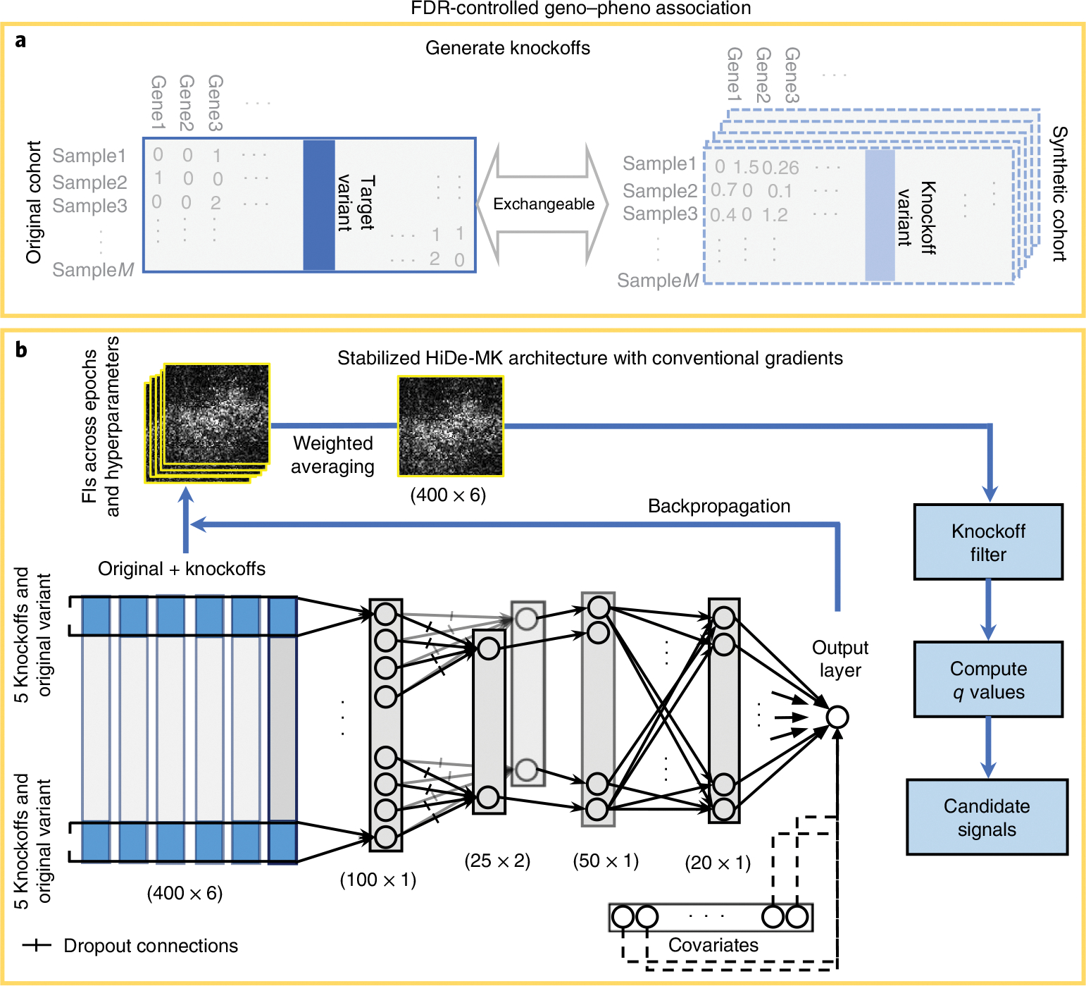
a,b, Knockoff feature generation (a; we generated five sets of knockoffs using SCIT in this study) and the proposed hierarchical deep learner along with aggregation of Fls and a knockoff filter for feature selection (b). We used two hierarchial layers to substantially decrease the size of the network. We also used an ELU activation function for better network performance. Gradients were used to measure Fls, which are monitored and collected for each epoch and each set of hyperparameters. The size of the Fls is the same as the input data. The obtained Fls were stabilized by weighted averaging and used to compute a $q$ value. Variants with $q$ values less than the target FDR level will be selected.

The proposed neural network includes two hierarchical layers (Fig. 1b), which are locally connected dense layers. The first layer concatenates each original feature and its multiple knockoffs as the input for each neuron, whereas the second concatenates adjacent genetic variants in a nearby region. This was inspired by recent advances for the gene/window-based analysis of WGS data, where multiple common and rare variants are grouped for improved power^30,31. The output of the second hierarchy includes multiple channels (filters) that help maximally learn the information of a local region and exploit the local correlation in each group. These two hierarchial layers substantially reduce the size of the parameter space compared with using standard dense layers. The resulting neurons are then fed into dense layers and then linked to the output layer together with additional covariates such as gender and principal components, which are used as controls for population stratifications (Fig. 1b).

The next step is to obtain the FIs, that is, the importance of each genetic variant. The influence of feature $x_i,i=1,\dots ,p$ on the response $\mathbf{y}\in {\mathbb{R}}^n$ is measured³² via the gradient for both true and knockoff features through the backpropagation (Fig. 1b). The gradient information is then summarized as FIs (see the Methods for details on how FIs are calculated). HiDe-MK hyperparameters were tuned based on a fivefold cross-validation. We then refitted the model to the whole data and calculated FIs for every epoch and every set of hyperparameters. We did not perform a train–test split because we focused on the feature selection, where sample size is critical for improved statistical power. Furthermore, the validity of the feature selection (that is, FDR control) is guaranteed by the knockoff inference, which does not require compution of FIs from held-out test data. Due to the random nature of fitting neural network models, and the identifiability issue that results from the large number of weight parameters, taking FIs from a single model can lead to unstable and random FIs. We therefore define the final FIs as an aggregation of FIs across epoch numbers and hyperparameters, which helps stabilize the proposed HiDe-MK. We demonstrated in both simulation studies and real data analyses that our approach—referred to as stabilized HiDe-MK—substantially reduced the variability and improved the stability of the FIs.

Once the FIs for original and knockoff features were obtained, a knockoff filter was applied to select causal features with controlled errors at different target FDR threshold values (for example, 0.10, 0.20; Fig. 1b). We used the knockoff filter for multiple knockoffs proposed by He and colleagues²⁶, which leverages multiple knockoffs for improved power, stability and reproducibility. We describe knockoff generation, network specifications (activation functions, hyperparameters, regularizations and so on), feature importance calculation and stabilization, and feature selection in detail in the Methods.

Stabilized HiDe-MK improved power with controlled FDR.

We performed simulation studies for both quantitative and dichotomous outcomes (regression and classification tasks). The aim is to evaluate the FDR and power of the proposed stabilized HiDe-MK compared with several conventional methods such as support vector machines for classification (SVM) and regression (SVR), least absolute shrinkage and selection operator (Lasso), ridge regression (Ridge) and DeepPINK^33,34. For a fair comparison, all methods are based on the knockoff inference that controls the FDR. Different methods represent different calculations of FIs. The proposed stabilized HiDe-MK, DeepPINK, Ridge, SVM, SVR and Lasso are equipped with five sets of knockoffs that are generated by the SCIT method proposed in KnockoffScreen²⁶.

For simulating the sequence data, each replicate consists of 10,000 individuals with genetics data on 2,000 variants from a 200 kb region, simulated using the haplotype dataset in the SKAT package³⁵ to mimic the linkage disequilibrium structure of European ancestry samples. We restrict the simulation studies to common (minor allele frequency $\left(\mathrm{M}\mathrm{A}\mathrm{F}\right)\ge 1\mathrm{\%}$) and rare ($\mathrm{M}\mathrm{A}\mathrm{F}<0.01$, minor allele count $\left(\mathrm{M}\mathrm{A}\mathrm{C}\right)\ge 10$) genetic variants. Ultra-rare variants with $\mathrm{M}\mathrm{A}\mathrm{C}<10$ are excluded from the experiments^3,31. These restrictions result in 400–500 variants as input features for each replicate. The quantitative and dichotomous outcomes are simulated as a nonlinear function of the genetic variants. Simulation details are described in the Methods.

For each replicate, the empirical power is defined as the proportion of detected true signals among all causal signals, whereas the empirical FDR is defined as the proportion of false signals among all detected signals. Based on 500 replicates, we report the average empirical power and observed FDR at different target FDR levels from 0.01 to 0.20, with a step size of 0.01 (Fig. 2). We also report the standard deviation of the estimated power in Supplementary Table 1. The proposed method exhibits higher power (for example, target $\mathrm{F}\mathrm{D}\mathrm{R}\ge 0.10$; Fig. 2) than its counterparts. The second-best model is Lasso-MK, while SVM and SVR are highly competitive. Stabilized HiDe-MK exhibited a higher power than other linear alternatives because a DNN is able to dynamically incorporate the nonlinear effects without having to specify them explicitly. We found that DeepPINK exhibits lower power than stabilized HiDe-MK, although both methods are nonlinear. One plausible explanation is that DeepPINK with a ReLU activation function suffers from the vanishing gradients problem. We evaluated the impact of activation functions on power and present the results in Supplementary Fig. 2. The results demonstrated that the ELU activation function used in the proposed method results in higher power than other alternatives. We also evaluated same methods with single knockoff (as in KnockoffZoom, Sesia et al.²⁴ and DeepPink, Lu et al.²⁵) and present the results in Supplementary Fig. 3. Compared with single-knockoff-based methods, we show that integration of the multiple knockoffs achieves improved power. This is because a single knockoff has diminished power when the number of signals is small and the target FDR is low, which is referred to as a detection threshold issue³⁶. To further validate whether our proposed method could control the FDR in the presence of ultra-rare variants, we conducted another experiment without the $\mathrm{M}\mathrm{A}\mathrm{C}\ge 10$ filter (Supplementary Fig. 4); the results showed that the FDR remains valid.

Fig. 2 |. Power and FDR comparison.

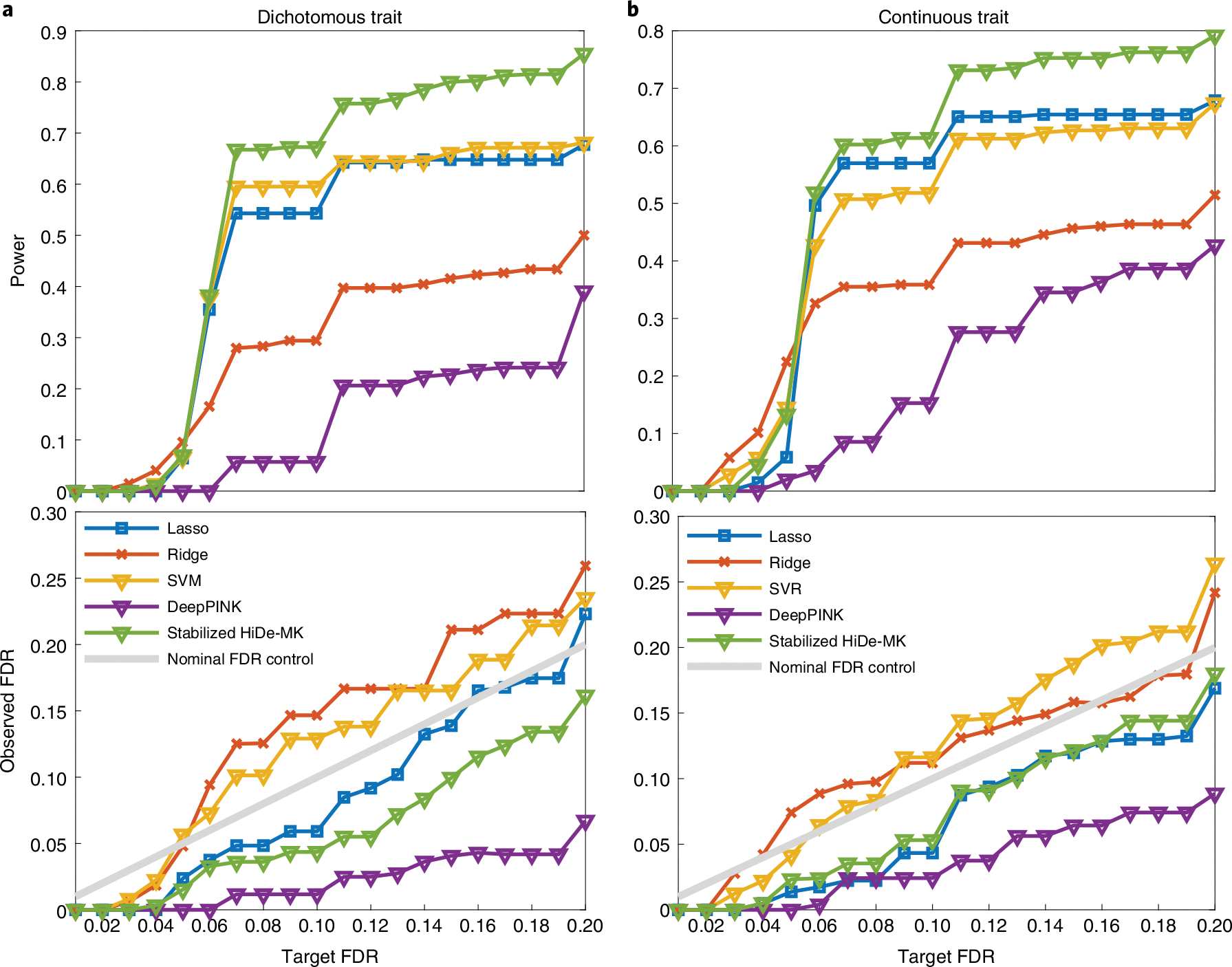
a,b, The observed power and FDR for dichotomous (a) and quantitative traits (b) with varying target FDRs from 0.01 to 0.20. Stabilized HiDe-MK, stabilized version of hierarchical deep neuro-network with multiple knockoffs; DeepPINK, deep feature selection using paired-input nonlinear knockoffs. All methods are equipped with five sets of knockoff features.

Application of stabilized HiDe-MK to GWAS.

The main goal of WGS studies is to identify genetic variants associated with certain disease phenotypes, referred to as GWAS. We applied our method to two real data problems to study AD genetics. For comparison, we considered feature selection in Lasso with multiple knockoffs, which is an extension of KnockoffZoom²⁴ that utilizes multiple knockoffs. See the Methods for details on dataset preparation.

Confirmatory-stage analysis of candidate regions.

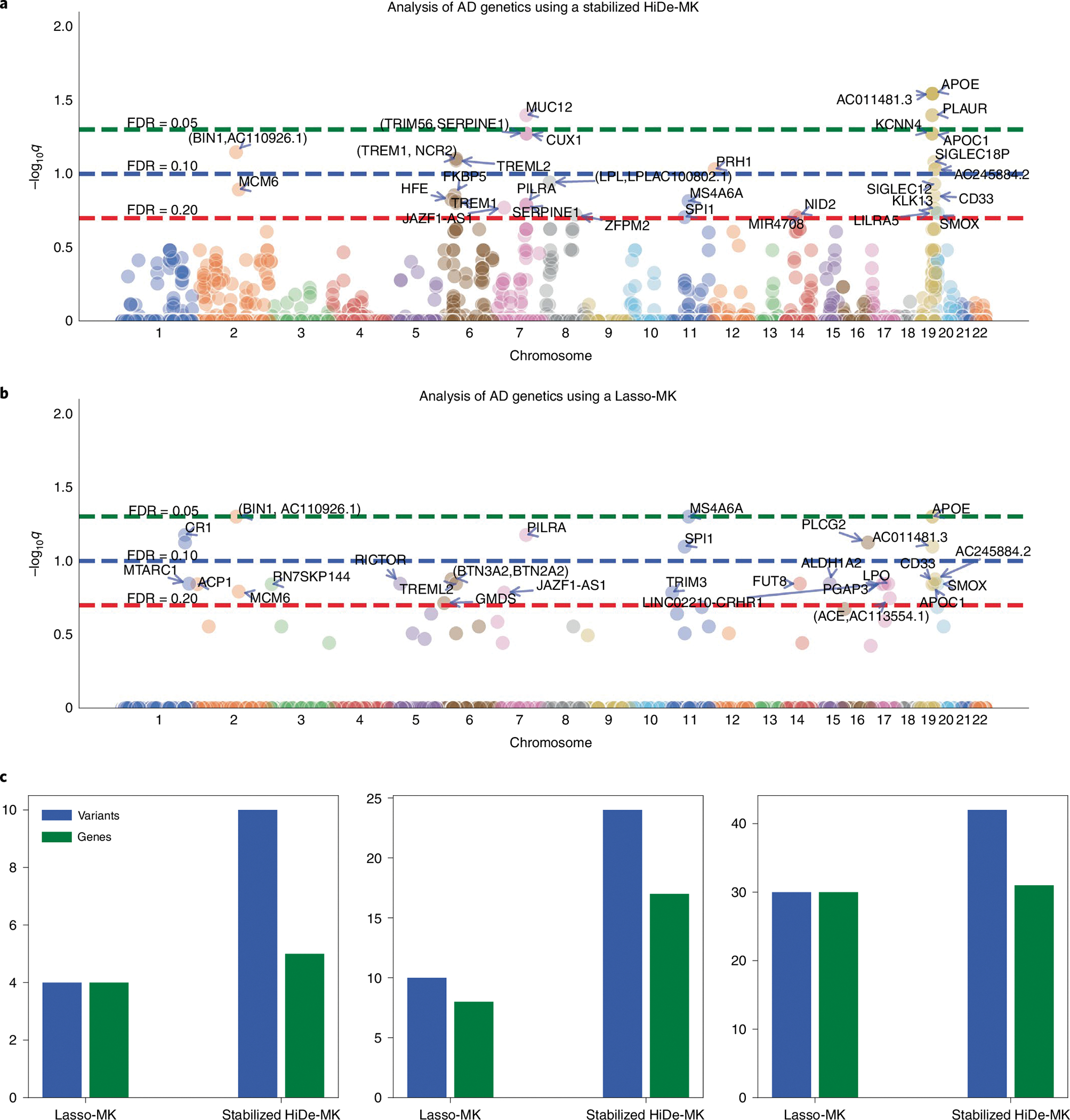
In the first task, referred to as a confirmatory-stage analysis, we aim to study candidate regions identified by previous exploratory-stage analyses to pin down the final discoveries that allow for nonlinear effects³⁷. We applied stabilized HiDe-MK to the confirmatory stage using a cohort of 10,797 clinically diagnosed AD cases and 10,308 healthy controls. The candidate regions include 472 loci associated with AD (394 from the UK biobank analysis by He et al.⁸; 78 from previous GWAS) and with a 5 kb window centered on each locus^38,39. The final dataset for the confirmatory stage includes 21,105 samples with 11,662 genetic variants. We present the results in Fig. 3. We observed that stabilized HiDe-MK identified 35 AD-associated genetic variants that meet the target FDR of 0.10, corresponding to 27 proximal genes (Supplementary Table 2). By contrast, Lasso-MK identifies 24 AD-associated variants that correspond to 26 proximal genes at a target FDR of 0.10. A further comparison with DeepPINK-MK with a ReLU activation function is displayed in Supplementary Fig. 5. We also performed conventional marginal association tests in GWAS and presented the results in Supplementary Fig. 6. Based on the standard GWAS with a 5 × 10⁻⁸ threshold, we observed that the marginal tests identify fewer independent loci than the joint models with conditional tests; for example, they missed the signals in chr7 (CASTOR3, EPHA1), chr8 (SHARPIN), chr15 (ADAM10), chr16 (KAT8), chr18 (ABCA7) and so on.

Fig. 3 |. Confirmatory-stage analysis of candidate regions.

a,b, Manhattan plots for a stabilized HiDe-MK (a) and a Lasso-MK (b). Each data point represents a genetic variant. The dashed horizontal lines indicate target FDRs. c, The number of identified genes and variants for stabilized HiDe-MK and Lasso-MK at target FDRs of 0.05 (left), 0.10 (middle) and 0.20 (right).

Functionally informed analysis of pQTLs.

In the second task, referred to as functionally informed analysis, we aim to identify protein quantitative trait loci (pQTL genetic variants that increase/decrease protein abundance level) that are also associated with the risk of AD. This analysis aims to discover novel variants associated with AD, which already have some functional support such as being associated with protein abundance level, such that we can translate the data-driven discovery into mechanistic insights. Specifically, we curated pQTLs recently identified by Ferkingstad et al.⁴⁰ for a total of 8,461 variants across the genome. We applied the proposed method to the same 21,105 samples, and present the results in Fig. 4. We observed that stabilized HiDe-MK identified 24 AD-associated genetic variants that meet the target FDR of 0.10, corresponding to 17 proximal genes (Supplementary Table 3 and Fig. 4). By contrast, Lasso-MK identifies ten AD-associated variants corresponding to nine proximal genes at target FDR 0.10.

Fig. 4 |. Functionally informed analysis of pQTLs.

a,b, Manhattan plots for a stabilized HiDe-MK (a) and a Lasso-MK (b). Each dot point represents a genetic variant. The dashed horizontal lines indicate target FDRs of 0.05 (left), 0.10 (middle) and 0.20 (right). c, The number of identified genes and variants for stabilized HiDe-MK and Lasso-MK at different target FDRs.

It is worth noting the development of the novel architecture was undertaken on simulations using the haplotype dataset in the SKAT package, which is independent of the real data application. The superior performance of stabilized HiDe-MK in this real data analysis illustrates the generalizability of the proposed architecture. Overall, the proposed method is the first to embark on deep learning methods to genetic data that can robustly detect putative causal variants of a trait. Both examples (the confirmatory analysis and the functionally informed discovery stage) demonstrated the superior performance of the methods. Future work on distributed learning that further optimizes the memory use and computing time will be necessary to apply the model to large-scale, unbiased whole genome screening.

Discussion

In this study we proposed an interpretable DNN, named stabilized HiDe-MK, for the identification of putative causal genetic variants in WGS studies. We took advantage of the localizable structure of genetic variants through hierarchical layers in the architecture of DNN to seamlessly reduce the size of the DNN. We further employed knockoff framework with multiple set of knockoffs to rigorously control the FDR during feature selection. Although the underlying goal is to identify putative causal variants, we observed a non-trivial randomness in the selected genetic variants. Two different runs of any DNNs including HiDe-MK, from the same hyperparameters, led to different candidate variants, which we found concerning. To stabilize identified signals, we proposed an ensemble method aggregating the FIs extracted from different epochs and hyperparameters, which allows us to confidently determine the final selected features with much less variance. With a thorough experiment conducted on two simulation datasets, validated for both regression and classification, on both common and rare variants, we empirically showed the proposed method improves power with a controlled FDR and substantially increases the stability of FIs (Fig. 5). For real data analysis, we applied stabilized HiDe-MK to two tasks; the confirmatory stage of a GWAS, and functionally informed analysis of pQTLs. Stabilized HiDe-MK identified several genetic variants that were missed by a linear model (Lasso with multiple knockoffs, Lasso-MK). This may shed light on the discovery of additional risk variants using sophisticated DNNs in future genetic studies.

Fig. 5 |. Stabilized HiDe-MK improves the stability of Fls compared with a single HiDe-MK run.

a, The correlation matrix of ten different runs of HiDe-MK with identical learning hyperparameters reveals a drastic randomness in every run. b, The correlation matrix of ten different stabilized HiDe-MK runs reveals strong correlation of Fls in every run. c, We also measured the stability of Fls across epoch numbers in terms of knockoff feature $W$ statistics for both HiDe-MK and stabilized HiDe-MK.

Our current analysis is based on the SCIT knockoff generator that assumes a homogenous population. Extensions to other ancestries, especially to minority population or admixed population, are particularly challenging. Previous empirical studies show that valid FDR can be achieved for admixed population by: (1) generating knockoffs based on the corresponding admixed population data and (2) adjusting for ancestry principal components as covariates²⁶. However, it has been shown that new knockoff generators that account for population structure are required to better address population stratification⁴¹. Future incorporation of such new knockoff generators that directly account for population structure can further improve the performance of the proposed method.

We observed the prediction accuracy by itself is inadequate as a single criterion for model training if the goal is feature selection. Models with similar prediction accuracy, but different FIs, can have different power in terms of feature selection. For example, Lasso and Ridge regression are both linear models that can lead to similar prediction accuracy, but the FIs (defined by regression coefficients) can be drastically different (for example, Lasso coefficients are sparse, but Ridge coefficients are dense) and subsequently the power can be very different (Fig. 2). Currently, we defined gradients in neuro-networks as FIs. Future study on the optimal choice of FIs in neuro-networks would be of great interest.

Last, we found that it remains challenging to fit a DNN to include all genetic variants in the genome, although substantial improvement has been made in the proposed architecture to improve the computational efficiency compared to usual neural networks (Fig. 6). Hence, the current analysis focuses on method comparisons using a replication dataset. It will be of interest to develop distributed learning that further optimizes the memory use and computing time in the future, such that DNN can be efficiently applied to large scale whole genome analysis for genome-wide causal variants discovery.

Fig. 6 |. The hierarchical layers improve computational efficiency.

The comparison was measured on data with 21,105 individuals, 1,000 randomly selected genetic variants, and five knockoffs per variant. a, The number of weights of the three models. b, The averaged time per epoch. c, The number of activation functions.

Methods

Simulated data to evaluate empirical FDR and power.

Extensive experiments were performed to evaluate the empirical FDR and power. The initial genetics data for performing simulations comprised 10,000 individuals, with 2,000 genetic variants drawn from a 200 kb region, based on a coalescent model (COSI) mimicking linkage disequilibrium structure of European ancestry⁴². Simulations were devised for both rare and common variants with $\mathrm{M}\mathrm{A}\mathrm{C}>10$. We followed the settings in KnockoffScreen²⁶ with slight modification. Strong correlation among variants (known as tightly linked variants) may make it difficult for learning methods to distinguish a causal genetic variant from its highly correlated counterpart (see Sesia et al.⁴³). We therefore only picked variants from each tightly linked cluster in the presence of strong correlations. Specifically, hierarchical clustering is first applied to variants to not allow two clusters to share a cross-correlations of greater than 0.75; variants from each cluster are then randomly chosen as candidates and are included in our simulation studies²⁶. We set four variants in a 200 kb region as causal variants. We evaluated quantitative and dichotomous traits generated by:

$$\mathrm{Q}\mathrm{u}\mathrm{a}\mathrm{n}\mathrm{t}\mathrm{i}\mathrm{t}\mathrm{a}\mathrm{t}\mathrm{i}\mathrm{v}\mathrm{e}\mathrm{t}\mathrm{r}\mathrm{a}\mathrm{i}\mathrm{t}:Y_i=X_{i1}+Cf\left({\beta }_1{g}_1+\dots +{\beta }_s{g}_s\right)+{\epsilon }_i,$$

$$\mathrm{D}\mathrm{i}\mathrm{c}\mathrm{h}\mathrm{o}\mathrm{t}\mathrm{o}\mathrm{m}\mathrm{o}\mathrm{u}\mathrm{s}\mathrm{t}\mathrm{r}\mathrm{a}\mathrm{i}\mathrm{t}:g\left({\mu }_i\right)={\beta }_0+X_{i1}+\mathrm{C}\mathrm{f}\left({\beta }_1{g}_1+\dots +{\beta }_s{g}_s\right)$$

where $X_{i1}\sim N(0,1)$, ${\epsilon }_i\sim N(0,2)$ and they are all independent; $\left(g_1,\dots ,g_s\right)$ are selected risk variants; $g\left(x\right)=\mathrm{l}\mathrm{o}\mathrm{g}x/\mathrm{l}\mathrm{o}\mathrm{g}(1-x)$; and ${\mu }_i$ is the conditional mean of the ith target. For the dichotomous trait, ${\beta }_0$ is chosen to have a prevalence of 0.10. The reason for this choice is that, in the USA, the study of a national representative sample of people aged > 70 years yielded an AD prevalence of 0.097. We therefore chose 0.1 to mimic a similar level of disease prevalence⁴⁴. The effect ${\beta }_j=\frac{a}{\sqrt{2m_j\left(1-m_j\right)}}$, where $m_j$ is the MAF for the jth variant. Parameter $a$ is defined such that the ${\beta }_1^{2}var\left(g_1\right)+\dots +{\beta }_s^{2}var\left(g_s\right)=0.2$ for the dichotomous trait and 0.04 for the quantitative trait. The choice of ${\beta }_j$ up-weights the effect size of rare variants. To mimic the real data scenario with both risk variants and protective variants, we set ${\beta }_1$ as negative and the others as positive. We also considered the nonlinear effect of the causal variants. We defined $f\left(x\right)=x^2$ and $C=2$ for both traits. This quadratic function corresponds to a nonlinear function that includes pairwise interactions that reflect the complex nonlinear effects of genetic variants. The aim is to identify signal variants and allow for nonlinear effects for improved power. With this set-up, the number of genetic variants including both common and rare variants is in the 400 to 500 range. We generate 500 replicates for each trait and report the average FDR and average power at different target FDR thresholds. For the dichotomous trait, the proposed model achieves an average validation area under the curve (AUC) of 0.565 (across 500 replicates), which is lower than the AUC that a single APOE region can achieve in AD genetics (0.65; Escott-Price et al.⁴⁵). For continuous trait, the proposed model achieves an average validation $R^2$ of 0.1269 (across 500 replicates), similar to the heritability explained by well-known AD loci (Sierksma et al.¹). We chose these low $\mathrm{A}\mathrm{U}\mathrm{C}/R^2$ values to reasonably mimic those observed in real AD genetic studies, in which the signal-to-noise ratio is low and the heritability explained by each variant is small. We used the R package GLMNET³³ to implement Lasso and Ridge regressions, and the R package LibLineaR³⁴ to implement SVR and SVM. The results illustrated that the statistical power remains high to detect small effect sizes, especially when it is compared with alternative methods.

Genetic data for AD.

We queried 45,212 individual genotypes from 28 cohorts⁴⁶ genotyped on genome-wide microarrays and imputed at high resolution on the basis of the reference panels from TOPMed using the Michigan Imputation Server⁴⁷. Phenotypic information and genotypes were obtained from publicly released GWAS datasets assembled by the Alzheimer’s Disease Genetics Consortium (ADGC), with the phenotype and genotype ascertainment described elsewhere^48–58. The exact cohorts used correspond with the replication data imputed in Le Guen and colleagues⁴⁶. We restricted our analysis to European ancestry individuals. After quality control, restricting to case/control status, pruning for duplicates of variants, and the third-degree relatedness, 21,105 unique individuals remained for the analysis.

For the confirmatory-stage analysis of the candidate regions, we considered 78 candidate variants from previous GWAS listed in Andrews et al.⁵⁹ and 394 candidate regions identified by a UK Biobank analysis using KnockoffScreen²⁶. We also included genetic variants in the neighbouring 5 kb of each candidate variant/region. The final dataset consists of 21,105 subjects and 11,662 variants. It is worth mentioning that the UK Biobank data (obtained in the United Kingdom) and the 10,797/10,308 case-control dataset (obtained in the United-States) are fully independent^60,61. However, the ADGC case-control dataset may potentially overlap with existing AD GWAS in which the additional 78 loci were taken. We focus on the confirmatory stage that includes all existing AD loci for the method comparisons in this paper. We considered the pQTLs identified by Ferkingstad and colleagues for the functionally informed analysis of pQTLs⁴⁰. The final dataset consists of 21,105 subjects and 8,461 variants.

Samples used in this manuscript are derived from the replication set imputed on the TOPMed reference panel and described in a work by Le Guen and colleagues⁶². We used gender, and ten principal components as covariates. The reason to exclude age as a covariate is that the reported age for cases (age-at-onset) is on average lower than the age of controls (age-at-visit) in non-population-based studies. Hence, in a frequently used GWAS model such as a logistic regression, if the covariate age is on average lower for cases than for controls, then the model will infer a negative effect of age on disease risk, that is, AD risk would decrease with older age. This is an incorrect assumption as AD risk increases with age. The incorrect age adjustment thus leads to statistical power loss⁶². This is notably the case in the Alzheimer’s Disease Sequencing Project (ADSP) and ADGC data (case-control design dataset) used in our study. Details on quality control, ancestry determination and pruning for sample relatedness can be found in Supplementary Section 1.

The knockoff framework.

Controlling the FDR when performing variable selection can be accomplished by the knockoff framework. With this purpose, a set of variants (so called knockoffs denoted by $\tilde{X}\in {\mathbb{R}}^{n\times p}$ with the same size of the original input $X\in {\mathbb{R}}^{n\times p}$) should be created, where $p$ accounts for genetic variants and $n$ for the total number of individuals. As knockoffs are conditionally independent of the response vector $\mathbf{y}\in {\mathbb{R}}^n$, we expect those true variables to exhibit higher association with $\mathbf{y}\in {\mathbb{R}}^n$ than their knockoff counterparts. The knockoffs framework can be summarized in four steps:

1. Generate multiple knockoffs for each true variant.

2. Calculate the FIs for the original variants and the knockoff variants; FIs are assigned by a data-driven learning model.

3. Calculate the feature statistic by contrasting FIs between the original and their knockoff counterparts.

4. Apply a knockoff filter to select variants with a $\text{q}$ value less than the target FDR level.

We explain these steps in the following section.

Generate multiple knockoff variables.

To generate knockoff variants $\tilde{X}\in {\mathbb{R}}^{n\times p}$, two properties should be deemed: (1) $\tilde{X}\in {\mathbb{R}}^{n\times p}$ is independent of $\mathbf{y}\in {\mathbb{R}}^n$ conditional on $X\in {\mathbb{R}}^{n\times p}$; and (2) $X$ and $\tilde{X}$ are exchangeable²². With this set-up, knockoff variants can serve as control variables for feature selection. There are two limitations for a single knockoff procedure: (1) a single knockoff is limited by the detection threshold $\left[\frac{1}{\alpha }\right]$, which is the minimum number of independent rejections that are needed to detect any association³⁶; (2) a single knockoff is not stable in terms of the selected sets of features, that is, two different runs of a single knockoff may generate different sets of features and lead to different selected features. To reduce the randomness issue and improve power, we used the efficient SCIT algorithm proposed by He et al.²⁶ to generate multiple knockoffs that are simultaneously exchangeable. Algorithm 1 shows the main steps of the SCIT algorithm, which yield a sequence of random variables obeying the exchangeability property.

Algorithm 1.

Sequential conditional independent tuples (multiple knockoffs)

$j=1$

while $j\le p$ do

Sample ${\tilde{\mathbf{x}}}_j^1,\dots ,{\tilde{\mathbf{x}}}_j^M$ independently from $ℒ\left({\mathbf{x}}_j\mid {\mathbf{x}}_{-j},{\tilde{\mathbf{x}}}_{1:j-1}^1,\dots ,{\tilde{\mathbf{x}}}_{1:j-1}^M\right)$

$j=j+1$

End

where $ℒ\left({\mathbf{x}}_j\mid {\mathbf{x}}_{-j},{\tilde{\mathbf{x}}}_{1:j-1}^1,\cdots ,{\tilde{\mathbf{x}}}_{1:j-1}^M\right)$ is the conditional distribution of ${\mathbf{x}}_j$ given ${\mathbf{x}}_{-j},{\tilde{\mathbf{x}}}_{1:j-1}^1,\cdots ,{\tilde{\mathbf{x}}}_{1:j-1}^M$ where $-j$ indicates the variable ${\mathbf{x}}_j$ is excluded and $M$ is the total number of knockoffs.

Calculate the FIs.

For a FCNN, DeepPINK²⁵ used the multiplication of weight parameters from all layers as FIs. In DNNs with more complicated architectures, the multiplication of tensorial weights is not well-defined. To compute FIs in the proposed hierarchical DNN, we define FIs using the gradients of output $\mathbf{y}\in {\mathbb{R}}^n$ with respect to inputs $X\in {ℝ}^{n\times p\times (M+1)}$; that is, the importance of feature ${\mathbf{x}}_j$ on the response $\mathbf{y}\in {\mathbb{R}}^n$ is measured by the local sensitivity of the predictive function to that feature. This is represented by a vector $𝒯=\left({𝒯}_1,{𝒯}_2,\dots ,{𝒯}_p\right)$, of length $p$, in which ${𝒯}_j=\mathbb{E}\left[\partial f\left(X\right)/\partial X_j\right]$, where $\mathbb{E}$ represents the expectation with respect to the joint distribution $\left(y,X_1,\dots ,X_p\right)$ and $f$ represents the DNN. To compute this, we take the gradients for the input data $X\in {\mathbb{R}}^{n\times p\times (M+1)}$, giving a gradient tensor $\mathbb{T}\in {\mathbb{R}}^{n\times p\times (M+1)}$, where $M$ is the number of knockoffs. We then take the average over samples, which leads to the final FI matrix $T\in {\mathbb{R}}^{p\times (M+1)}$. The jth row of $T\in {\mathbb{R}}^{p\times (M+1)}$ contains the FIs of original and knockoffs for the jth feature. Obtaining FIs with gradient information is architecture-independent; regardless of the neural network’s architecture, the gradients of output with respect to inputs can be easily monitored and calculated.

Calculate the knockoff feature statistic.

Assume $T=\left[T^0,T^1,\dots ,T^M\right]$ is the matrix of FIs, where $T^0\in {\mathbb{R}}^p$ represents FIs for the original variants and the rest are for $M$ sets of knockoffs. For the selection of important variants, the absolute values of FIs (or absolute values of gradients) are passed to the knockoff selection procedure. For a single knockoff-based model, $W_j=\left|T_j^0\right|-\left|T_j^1\right|$. Intuitively, the original variants with higher FIs than its knockoffs are more likely to be causal. For multiple knockoffs, we used a multiple-knockoff feature statistic proposed by He and co-workers²⁶. Two metrics ${\kappa }_j$ and ${\tau }_{\mathrm{j}}$ are calculated for each feature $1\le j\le p$ as follows

$${\kappa }_j=\underset{0\le m\le M}{\mathrm{a}\mathrm{r}\mathrm{g}\mathrm{m}\mathrm{a}\mathrm{x}}{T}_j^m,1\le j\le p,m\in \{0,1,\dots ,M\}$$

$${\tau }_j=T_j^{\left(0\right)}-\underset{1\le m\le M}{\mathrm{m}\mathrm{e}\mathrm{d}\mathrm{i}\mathrm{a}\mathrm{n}}{T}_j^{\left(m\right)}$$

Where ${\kappa }_j$ denotes the index of the original (denoted as 0 ) or the knockoff feature that has the largest importance score; ${\tau }_j$ denotes the difference between the largest importance score $T_j^{\left(0\right)}$ and the median of the remaining scores. The indexing in parenthesis refers to the ordered sequence of FIs in descending order; $T_j^{\left(0\right)}$ is therefore the largest FI for the jth feature, which can be either for the original feature or one of the knockoffs. The feature statistic is defined as

$$W_j=\left(T_j^0-\underset{1\le m\le M}{\mathrm{m}\mathrm{e}\mathrm{d}\mathrm{i}\mathrm{a}\mathrm{n}}{T}_j^m\right)I_{T_j^0\ge }\underset{1\le m\le M}{\mathrm{m}\mathrm{a}\mathrm{x}} T_j^m$$

It has been empirically shown that the knockoff statistics with median substantially improves stability and reproducibility of knockoffs²⁶.

Knockoff filter and Q-statistics for feature selection.

The last step of knockoff framework is feature selection with $\mathrm{F}\mathrm{D}\mathrm{R}\le \alpha$, where $\alpha$ is a pre-defined bound for FDR, known as target FDR level. For a single knockoff, the feature statistic is defined as, $W_j=\left|{\mathrm{T}}_j^0\right|-\left|{\mathrm{T}}_j^1\right|$ and the knockoff threshold $\hat{\tau }$ is chosen as follows²²:

$$\hat{\tau }=\mathrm{m}\mathrm{i}\mathrm{n}\left\{t>0:\frac{1+\#\left\{j:W_j\le -t\right\}}{\#\left\{j:W_j\ge t\right\}}\le \alpha \right\},$$

For multiple knockoffs,

$$\hat{\tau }=\mathrm{m}\mathrm{i}\mathrm{n}\left\{t>0:\frac{\frac{1}{M}+\frac{1}{M}\#\left\{{\kappa }_j\ge 1,{\tau }_j\ge t\right\}}{\#\left\{{\kappa }_j=0,{\tau }_j\ge t\right\}}\le \alpha \right\}.$$

Variants with $W_j\ge \hat{\tau }$ are selected. Equivalently, a knockoff $Q$ value can be computed as

$$q_j=\underset{t\le {\tau }_j}{\mathrm{m}\mathrm{i}\mathrm{n}} \frac{\frac{1}{M}+\frac{1}{M}\#\left\{j:{\kappa }_j\ne 0,{\tau }_j\ge t\right\}}{\#\left\{j:{\kappa }_j=0,{\tau }_j\ge t\right\}}$$

for variants with statistics $\kappa =0$, and $q_j=1$ for variants with $\kappa \ne 0$. Selecting variants/windows with $W_j>\hat{\tau }$ is equivalent to selecting variants/windows with $q_j\le \alpha$.

The advantage of the multiple-knockoff selection procedure is the new offset term $\frac{1}{M}$ (averaging over $M$ knockoffs) that enables us to decrease the threshold of minimum number of rejections from $\frac{1}{\alpha }$ to $\frac{1}{M\alpha }$, leading to an improvement in the power. The use of median in the calculation of $W$ improves the stability.

The proposed hierarchical deep learning structure.

Conventional FCNNs can be computationally intensive for genetic data due to the massive number of genetic variants $p$. Furthermore, to control FDR, the inclusion of the knockoff data adds more to both computational time and resources. Knowing the fact that the first layers of a deep learner include many weight parameters and it is essential to control the size of the neural network in its first layers; hierarchical deep neural networks are used to exponentially reduce the size of a DNN^63–66. Assume that the number of neurons corresponding to each variant is $(M+1)\times p$, where $M$ is the number of knockoffs (set to five in our experiments). In our proposed hierarchical deep learner, we group every original feature and its knockoffs in the first layer to a single neuron in the next layer through a nonlinear activation function. Hence, the size of neurons in the next layer reduces to $p$ neurons. We call this combination between two feature types as feature-wise hierarchy. Next, adjacent variants inherit similar traits and therefore one can take the variants of the adjacent regions into the same groups. Assume that the number of variants in each group is set to $\sigma >1$. Then every $\sigma$ neurons out of $p$ neurons in the second layer are grouped to a small set of $\theta$ neurons (channels) in the next layer. Hence, the number of neurons is further reduced to $\theta [p/\sigma ]$. We call this combination between features in the second layer as region-wise hierarchy. These are analogous to filters in a convolutional neural network. The architecture of the proposed HiDe-MK is illustrated in Fig. 1 and Supplementary Fig. 1. Also see Supplementary Fig. 7 for the impact of different numbers of kernel size on the observed FDR, power and the total number of weight parameters of HiDe-MK. In our experiments, the number of channels in the second hierarchical layer is set to 8. We present detailed model configurations in Supplementary Section 2.

Activation functions of HiDe-MK.

Deep learning consists of several layers in its structure, which learn the underlying structure of data through nonlinear activation functions. Although a sufficiently deep neural network structure can learn complex features of real-world applications, having several layers in the DNN structure introduce some challenges to training, such as the vanishing gradient problem and the saturation problem of activation functions⁶⁷. The ReLU is one of the most popular activation functions in deep learning²⁹ due to its outstanding performance and low computational cost compared with other activation functions such as the logistic sigmoid and the hyperbolic tangent⁶⁸. However, if the data fall into the hard zero negative part of the ReLU, many neurons will not be reactivated during the training process and its corresponding gradients are set to zero, which avoid the weight update. This issue is known as the dying ReLU problem. In our experiments, the ELU activation function exhibited the best performance among the other activation functions listed above. We tabulate a list of important activation functions In Supplementary Table 4. Results of FDR and power with unique activation functions (namely, ELU, Swish, GeLU and ReLU) are also displayed in Supplementary Fig. 2.

Stabilized FIs.

Interpretations of DNN methods are known to be fragile²⁰. In the application of HiDe-MK to the analysis of AD genetics, we observed that different HiDe-MK runs—with the same dataset, knockoff features, hyperparameters, epoch number and validation loss—lead to drastically different FIs and therefore produce different sets of selected features. This is plausibly due to the non-convexity of deep learning methods, which rely on random parameter initialization and stochastic gradient descent to reach a local optimum. The resulting gradient-based FIs thus tend to be stochastic. We present the randomness of FIs in Fig. 5a in terms of the correlation between FIs across ten HiDe-MK runs. HiDe-MK was applied to the aforementioned AD genetics data, with the knockoff features, hyperparameters and epoch number remaining identical in each run. Although the difference in validation loss is negligible, we observed a poor correlation $(<0.50)$ between different runs. This result suggests that direct application of conventional DNNs can give rise to misleading results. It also implies that the usual criteria for prediction cannot be directly applied to feature selection. A more consistent set of FIs is desirable to ensure rigorous inference.

To have a DNN method that reliably expresses the relationship between the genotype and phenotype, the neural network and its feature importance values should be stabilized, and the criteria to choose the optimal epoch number should be modified. We proposed an ensemble of FIs across epoch numbers and hyperparameters to improve the stability of HiDe-MK. Specifically, we first set the maximum epoch number and the search space for candidate hyperparameters. We conduct fivefold cross-validation over the epoch numbers and hyperparameters. For each combination of epoch number and hyperparameters, we compute the gradients as FIs and the validation loss. Finally, we calculate the weighted FIs, where the weights are defined by the validation loss. For the jth set of hyperparameters and the kth epoch number, the weight ${\psi }_{jk}$ is calculated as:

$${\psi }_{jk}=\frac{\mathrm{m}\mathrm{a}\mathrm{x}\left(\text{val\_loss}\right)-{\text{val\_loss}}_{jk}}{\mathrm{m}\mathrm{a}\mathrm{x}\left(\text{val\_loss}\right)-\mathrm{m}\mathrm{i}\mathrm{n}\left(\text{val\_loss}\right)}$$

Where val_loss is the validation loss. The stabilized FIs are eventually calculated as $\mathrm{F}\mathrm{I}={\sum }_{jk} {\psi }_{jk}{\mathrm{F}\mathrm{I}}_{jk}$. Intuitively, the proposed ensemble up-weights models with lower validation loss and vice versa. As the ensemble is embedded in the cross-validation of model training, it only requires fitting the model once without additional computational cost. We refer to this ensemble method as stabilized HiDe-MK. We present the empirical results in Fig. 5b. We observed a high correlation $(>0.95)$ between different stabilized HiDe-MK runs, where each run aggregates sets of FIs that are drawn from different epoch numbers and hyperparameters, demonstrating that the ensemble method helps stabilize FIs. This step of stabilization was crucial in our modelling as our goal was to report a credible set of AD-associated genes. Furthermore, we evaluated the stability of FIs across epoch numbers. For every epoch, we monitored the knockoff feature W statistics and calculated the correlation for every two consecutive epochs. We evaluate both HiDe-MK and its stabilized version (Fig. 5c). We observed a high correlation in FIs between two consecutive epochs as epoch number increases. We also observed that the stabilized HiDe-MK is more stable than HiDe-MK.

Aside from the randomness due to the stochastic nature of deep learning methods, many interpretable DNNs rely on a set of randomly generated ‘control’ features, such as the surrogate variables in SurvNet and the knockoff variables in the proposed methods. We also note that randomness brought by surrogate/knockoff variables may also hinder the interpretability. We propose using multiple knockoffs and a corresponding knockoff filter to stabilize the feature selection. A detailed comparison between multiple-knockoff and single-knockoff methods was discussed by He and colleagues²⁶.

The hierarchical layers improve computational efficiency.

The computational cost plays a key role in the application of deep learning methods to genetics data in the presence of knockoffs data, which multiply the number of input features. Deep learning methods that use several hidden layers in its structure can be computationally intensive. As the number of features increases, the network size in terms of the number of weight parameters and number of activations gets larger and, consequently, the computational burden increases. We compared three different learning methods to illustrate the importance of hierarchically structured DNNs: (1) a FCNN, that is, a neural network with one level of hierarchy (as in DeepPINK); and (2,3) a neural network with two levels of hierarchy. FCNN is a conventional DNN with three dense hidden layers. The one-level-hierarchy model uses an initial locally connected layer to join each original feature with its five knockoffs from input layer to the next layer, and this reduced set of neurons is connected to the remaining layers with the same architecture as FCNN. The two-levels-of-hierarchy model uses one more level of hierarchy than a one-level-hierarchy model to group adjacent genetic variants, replacing the corresponding dense layer.

We applied these methods to the genetic data consisting of 21,105 individuals and 11,662 genetic variants. The batch size and the number of epochs are set to 1,024 and 50 respectively. On our computing system (2.40 GHz Intel CPU and 128 GB of RAM), we noticed that experiments with FCNN causes an out-of-memory error due to the huge number of its weight parameters. We therefore limited our experiments to the random selection of only 1,000 genetic variants and their five set of knockoffs as a proof of concept. We ran these models 50 times and reported the average number of weights, computational time and the number of activations (see Fig. 6 for the results). A two-level hierarchy has two orders of magnitude fewer weight parameters in its architecture than a one-level hierarchy, and four orders of magnitude fewer than a FCNN that does not use any hierarchical layer (Fig. 6a). Figure 6b displays the averaged time per epoch for three counterparts: a two-level hierarchy is two times faster than one-level hierarchy, and 40 times faster than a FCNN. We also quantified the number of activations as it is also an important factor in measuring the model’s efficiency⁶⁹ and present the results in Fig. 6c. Again, a two-level hierarchy uses about 2- and 12-times-fewer activation functions than the one-level hierarchy and FCNN, respectively. DNNs with hierarchical layers are much more efficient than DNNs with dense layers. In terms of the memory usage, the peak memory use is, on average, 29.51 GB for a one-level hierarchy, 30.18 GB for a two-level hierarchy, and 31.05 GB for a FCNN.

Data availability

Alzheimer’s disease genetic cohort data can be obtained for approved research (see the description in the work by Le Guen and colleagues⁶²). Simulation datasets are available on our GitHub repository: https://github.com/Peyman-HK/De-randomized-HiDe-MK (ref.⁷⁰).

References

- 1.Sierksma A, Escott-Price V & De Strooper B Translating genetic risk of Alzheimer’s disease into mechanistic insight and drug targets. Science 370, 61–66 (2020). [DOI] [PubMed] [Google Scholar]
- 2.Visscher PM et al. 10 Years of GWAS discovery: biology, function, and translation. Am. J. Hum. Genet. 101, 5–22 (2017). [DOI] [PMC free article] [PubMed] [Google Scholar]
- 3.Lee S, Abecasis GR, Boehnke M & Lin X Rare-variant association analysis: study designs and statistical tests. Am. J. Hum. Genet. 95, 5–23 (2014) [DOI] [PMC free article] [PubMed] [Google Scholar]
- 4.Zuk O, Hechter E, Sunyaev SR & Lander ES The mystery of missing heritability: genetic interactions create phantom heritability. Proc. Natl Acad Sci. USA 109, 1193–1198 (2012) [DOI] [PMC free article] [PubMed] [Google Scholar]
- 5.Ma Y et al. Analysis of whole-exome sequencing data for Alzheimer disease stratified by APOE Genotype. JAMA Neurol. 76, 1099–1108 (2019). [DOI] [PMC free article] [PubMed] [Google Scholar]
- 6.Jun GR et al. Transethnic genome-wide scan identifies novel Alzheimer’s disease loci. Alzheimers. Dement. 13, 727–738 (2017). [DOI] [PMC free article] [PubMed] [Google Scholar]
- 7.Belloy ME et al. Association of klotho-VS heterozygosity with risk of Alzheimer disease in individuals who carry APOE4. JAMA Neurol. 77, 849–862 (2020). [DOI] [PMC free article] [PubMed] [Google Scholar]
- 8.He L et al. Exome-wide age-of-onset analysis reveals exonic variants in ERN1 and SPPL2C associated with Alzheimer’s disease. Transl. Psychiatry 11, 146 (2021). [DOI] [PMC free article] [PubMed] [Google Scholar]
- 9.Sims R, Hill M & Williams J The multiplex model of the genetics of Alzheimer’s disease. Nat. Neurosci. 23, 311–322 (2020). [DOI] [PubMed] [Google Scholar]
- 10.Costanzo M et al. A global genetic interaction network maps a wiring diagram of cellular function. Science 353, aaf1420 (2016). [DOI] [PMC free article] [PubMed] [Google Scholar]
- 11.Kuzmin E et al. Systematic analysis of complex genetic interactions. Science 360, eaao1729 (2018). [DOI] [PMC free article] [PubMed] [Google Scholar]
- 12.Phillips PC Epistasis — the essential role of gene interactions in the structure and evolution of genetic systems. Nat. Rev. Genet. 9, 855–867 (2008) [DOI] [PMC free article] [PubMed] [Google Scholar]
- 13.Moore JH & Williams SM Epistasis and its implications for personal genetics. Am. J. Hum. Genet. 85, 309–320 (2009). [DOI] [PMC free article] [PubMed] [Google Scholar]
- 14.Cordell HJ Detecting gene-gene interactions that underlie human diseases. Nat. Rev. Genet. 10, 392–404 (2009). [DOI] [PMC free article] [PubMed] [Google Scholar]
- 15.Scarselli F & Chung Tsoi A Universal approximation using feedforward neural networks: a survey of some existing methods, and some new results. Neural Netw. 11, 15–37 (1998) [DOI] [PubMed] [Google Scholar]
- 16.Koo PK & Ploenzke M Improving representations of genomic sequence motifs in convolutional networks with exponential activations. Nat. Mach. Intell. 3, 258–266 (2021) [DOI] [PMC free article] [PubMed] [Google Scholar]
- 17.Cao Y, Geddes TA, Yang JYH & Yang P Ensemble deep learning in bioinformatics. Nat. Mach. Intell. 2, 500–508 (2020) [Google Scholar]
- 18.Manifold B, Men S, Hu R & Fu D A versatile deep learning architecture for classification and label-free prediction of hyperspectral images. Nat. Mach Intell. 3, 306–315 (2021) [DOI] [PMC free article] [PubMed] [Google Scholar]
- 19.Song Z & Li J Variable selection with false discovery rate control in deep neural networks. Nat. Mach. Intell. 3, 426–433 (2021). [Google Scholar]
- 20.Ghorbani A, Abid A & Zou JY Interpretation of neural networks is fragile. In Proc. AAAI Conference on Artificial Intelligence Vol. 33 3681–3688 (AAAI, 2019); 10.1609/aaai.v33i01.33013681 [DOI] [Google Scholar]
- 21.Barber RF & Candès EJ Controlling the false discovery rate via knockoffs. Ann. Stat. 43, 2055–2085 (2015) [Google Scholar]
- 22.Candès E, Fan Y, Janson L & Lv J Panning for gold: ‘Model-X’ knockoffs for high dimensional controlled variable selection. J. R. Stat. Soc. B 80, 551–577 (2018) [Google Scholar]
- 23.Tibshirani R Regression shrinkage and selection via the Lasso. J. R. Stat. Soc. B 58, 267–288 (1996). [Google Scholar]
- 24.Sesia M, Katsevich E, Bates S, Candès E & Sabatti C Multi-resolution localization of causal variants across the genome. Nat. Commun. 11, 1093 (2020) [DOI] [PMC free article] [PubMed] [Google Scholar]
- 25.Lu YY, Fan Y, Lv J & Noble WS DeepPINK: reproducible feature selection in deep neural networks. In Proc. 32nd International Conference on Neural Information Processing Systems 8690–8700 (Curran Associates, 2018). [Google Scholar]
- 26.He Z et al. Identification of putative causal loci in whole-genome sequencing data via knockoff statistics. Nat. Commun. 12, 3512 (2021). [DOI] [PMC free article] [PubMed] [Google Scholar]
- 27.Lu L, Shin Y, Su Y & Karniadakis GE Dying ReLU and initialization: theory and numerical examples. Commun. Comput. Phys. 5, 1671–1706 (2020) [Google Scholar]
- 28.Clevert D-A, Unterthiner T & Hochreiter S Fast and accurate deep network learning by exponential linear units (ELUs). In International Conference on Learning Representations (ICLR, 2016). [Google Scholar]
- 29.LeCun Y, Bengio Y & Hinton G Deep learning. Nature 521, 436–444 (2015) [DOI] [PubMed] [Google Scholar]
- 30.He Z, Xu B, Buxbaum J & Ionita-Laza I A genome-wide scan statistic framework for whole-genome sequence data analysis. Nat. Commun. 10, 3018 (2019) [DOI] [PMC free article] [PubMed] [Google Scholar]
- 31.Li X et al. Dynamic incorporation of multiple in silico functional annotations empowers rare variant association analysis of large whole-genome sequencing studies at scale. Nat. Genet. 52, 969–983 (2020) [DOI] [PMC free article] [PubMed] [Google Scholar]
- 32.Dai C, Lin B, Xing X & Liu J False discovery rate control via data splitting. J. Am. Stat. Soc. 10.1080/01621459.2022.2060113 (2020) [DOI] [Google Scholar]
- 33.Tibshirani JF, Hastie T & Tibshirani R Regularization paths for generalized linear models via coordinate descent. J. Stat. Softw. 33, 1–22 (2010) [PMC free article] [PubMed] [Google Scholar]
- 34.Fan R-E, Chang K-W, Hsieh C-J, Wang X-R & Lin C-J LIBLINEAR: a library for large linear classification. J. Mach. Learn. Res. 9, 1871–1874 (2008) [Google Scholar]
- 35.Lee S, Zhao Z, Miropolsky L, Wu M SKAT: SNP-Set (Sequence) Kernel Association Test, R package, version 2.2.4. (2022)
- 36.Gimenez JR & Zou J Improving the stability of the knockoff procedure: multiple simultaneous knockoffs and entropy maximization. In Proc. 22nd International Conference on Artificial Intelligence and Statistics (AISTATS) (PMLR, 2018). [Google Scholar]
- 37.Ren Z, Wei Y & Candès E Derandomizing knockoffs. J. Am. Stat. Assoc. 10.1080/01621459.2021.196272 (2021) [DOI] [Google Scholar]
- 38.He Z et al. Genome-wide analysis of common and rare variants via multiple knockoffs at biobank scale, with an application to Alzheimer disease genetics. Am. J. Hum. Genet. 108, 2336–2353 (2021) [DOI] [PMC free article] [PubMed] [Google Scholar]
- 39.Shea J A, Fulton-Howard B & Goate A Interpretation of risk loci from genome-wide association studies of Alzheimer’s disease. Lancet Neurol. 19, 326–335 (2020) [DOI] [PMC free article] [PubMed] [Google Scholar]
- 40.Ferkingstad E et al. Large-scale integration of the plasma proteome with genetics and disease. Nat. Genet. 53, 1712–1721 (2021) [DOI] [PubMed] [Google Scholar]
- 41.Sesia M, Bates S, Candès E, Marchini J & Sabatti C False discovery rate control in genome-wide association studies with population structure. Proc. Natl Acad. Sci. USA 118, e2105841118 (2021). [DOI] [PMC free article] [PubMed] [Google Scholar]
- 42.Schaffner SF et al. Calibrating a coalescent simulation of human genome sequence variation. Genome Res 15, 1576–1583 (2005) [DOI] [PMC free article] [PubMed] [Google Scholar]
- 43.Sesia M, Sabatti C & Candès EJ Gene hunting with hidden Markoy model knockoffs. Biometrika 106, 1–18 (2019). [DOI] [PMC free article] [PubMed] [Google Scholar]
- 44.Plassman BL et al. Prevalence of dementia in the United States: the aging, demographics, and memory study. Neuroepidemiology 29, 125–132 (2007) [DOI] [PMC free article] [PubMed] [Google Scholar]
- 45.Escott-Price V, Shoai M, Pither R, Williams J & Hardy J Polygenic score prediction captures nearly all common genetic risk for Alzheimer’s disease. Neurobiol. Aging 49, 214.e7–214.e11 (2017). [DOI] [PubMed] [Google Scholar]
- 46.Guen Y. Le et al. A novel age-informed approach for genetic association analysis in Alzheimer’s disease. Alzheimer’s Res. Ther. 13, 72 (2021). [DOI] [PMC free article] [PubMed] [Google Scholar]
- 47.Das S et al. Next-generation genotype imputation service and methods. Nat. Genet. 48, 1284–1287 (2016) [DOI] [PMC free article] [PubMed] [Google Scholar]
- 48.Beecham GW et al. The Alzheimer’s disease sequencing project: study design and sample selection. Neurol. Genet. 3, e194–e194 (2017). [DOI] [PMC free article] [PubMed] [Google Scholar]
- 49.Weiner MW et al. The Alzheimer’s disease neuroimaging initiative: progress report and future plans. Alzheimers. Dement. 6, 202–211.e7 (2010). [DOI] [PMC free article] [PubMed] [Google Scholar]
- 50.Bennett DA et al. Overview and findings from the rush memory and aging project. Curr. Alzheimer Res. 9, 646–663 (2012). [DOI] [PMC free article] [PubMed] [Google Scholar]
- 51.Kunkle BW et al. Genetic meta-analysis of diagnosed Alzheimer’s disease identifies new risk loci and implicates β, tau, immunity and lipid processing Nat. Genet. 51, 414–430 (2019). [DOI] [PMC free article] [PubMed] [Google Scholar]
- 52.Kunkle BW et al. Novel Alzheimer disease risk loci and pathways in African American individuals using the African genome resources panel: a meta-analysis. JAMA Neurol. 78, 102–113 (2021). [DOI] [PMC free article] [PubMed] [Google Scholar]
- 53.Purcell S et al. PLINK: a tool set for whole-genome association and population-based linkage analyses. Am. J. Hum. Genet. 81, 559–575 (2007). [DOI] [PMC free article] [PubMed] [Google Scholar]
- 54.Price AL et al. Principal components analysis corrects for stratification in genome-wide association studies. Nat. Genet. 38, 904–909 (2006). [DOI] [PubMed] [Google Scholar]
- 55.Chen C-Y et al. Improved ancestry inference using weights from external reference panels. Bioinformatics 29, 1399–1406 (2013). [DOI] [PMC free article] [PubMed] [Google Scholar]
- 56.Auton A et al. A global reference for human genetic variation. Nature 526, 68–74 (2015). [DOI] [PMC free article] [PubMed] [Google Scholar]
- 57.Karczewski KJ et al. The mutational constraint spectrum quantified from variation in 141,456 humans. Nature 581, 434–443 (2020). [DOI] [PMC free article] [PubMed] [Google Scholar]
- 58.Taliun D et al. Sequencing of 53,831 diverse genomes from the NHLBI TOPMed Program. Nature 590, 290–299 (2021). [DOI] [PMC free article] [PubMed] [Google Scholar]
- 59.Andrews SJ, Fulton-Howard B & Goate A Interpretation of risk loci from genome-wide association studies of Alzheimer’s disease. Lancet Neurol. 19, 326–335 (2020). [DOI] [PMC free article] [PubMed] [Google Scholar]
- 60.Bycroft C et al. The UK Biobank resource with deep phenotyping and genomic data. Nature 562, 203–209 (2018). [DOI] [PMC free article] [PubMed] [Google Scholar]
- 61.Hechtlinger Y Interpretation of prediction models using the input gradient. Preprint at https://arxiv.org/abs/1611.07634 (2016).
- 62.Le Guen Y et al. A novel age-informed approach for genetic association analysis in Alzheimer’s disease. Alzheimers. Res. Ther. 13, 72 (2021). [DOI] [PMC free article] [PubMed] [Google Scholar]
- 63.Saha S et al. Hierarchical deep learning neural network (HiDeNN): an artificial intelligence (AI) framework for computational science and engineering. Comput. Methods Appl. Mech. Eng. 373, 113452 (2021) [Google Scholar]
- 64.Roy D, Panda P & Roy K Tree-CNN: a hierarchical deep convolutional neural network for incremental learning. Neural Netw. 121, 148–160 (2020) [DOI] [PubMed] [Google Scholar]
- 65.Kim J, Kim B, Roy PP & Jeong D Efficient facial expression recognition algorithm based on hierarchical deep neural network structure. IEEE Access 7, 41273–41285 (2019). [Google Scholar]
- 66.Xu Y et al. A hierarchical deep learning approach with transparency and interpretability based on small samples for glaucoma diagnosis. npj Digit. Med. 4, 48 (2021). [DOI] [PMC free article] [PubMed] [Google Scholar]
- 67.Glorot X & Bengio Y Understanding the difficulty of training deep feedforward neural networks. In Proc. 13th International Conference on Artificial Intelligence and Statistics (AISTATS) Vol. 9, 249–256 (JMLR, 2010). [Google Scholar]
- 68.LeCun YA, Bottou L, Orr GB & Müller K-R in Neural Networks: Tricks of the Trade (eds. Müller K-R et al.) 2nd edn, 9–48 (Springer, 2012); 10.1007/978-3-642-35289-8_3 [DOI] [Google Scholar]
- 69.Jha NK, Mittal S & Mattela G The ramifications of making deep neural networks compact. Preprint at https://arxiv.org/abs/2006.15098 (2020).
- 70.Peyman-HK/Stabilized-HiDe-MK: Stabilized HiDe-MK (Zenodo, 2022); 10.5281/zenodo.6872386 [DOI] [Google Scholar]
Associated Data
This section collects any data citations, data availability statements, or supplementary materials included in this article.
Supplementary Materials
Data Availability Statement