Plants sum and subtract stimuli over different timescales

Significance

Plants are sessile decentralized systems with no brain or neural system, and very little is known regarding how they quantify external stimuli. We experimentally probe the dependence of gravitropic responses of wheat coleoptiles on the presence of previous stimuli, revealing how coleoptiles integrate multiple stimuli over time. We report quantitative evidence that plants effectively respond not only to sums of stimuli but also to differences between stimuli, over different timescales. This finding advances our understanding of how plants negotiate their environment since the ability of organisms to subtract stimuli over time is crucial in order to compare signals and is at the basis of navigation and active sensing.

Abstract

Mounting evidence suggests that plants engage complex computational processes to quantify and integrate sensory information over time, enabling remarkable adaptive growth strategies. However, quantitative understanding of these computational processes is limited. We report experiments probing the dependence of gravitropic responses of wheat coleoptiles on previous stimuli. First, building on a mathematical model that identifies this dependence as a form of memory, or a filter, we use experimental observations to reveal the mathematical principles of how coleoptiles integrate multiple stimuli over time. Next, we perform two-stimulus experiments, informed by model predictions, to reveal fundamental computational processes. We quantitatively show that coleoptiles respond not only to sums but also to differences between stimuli over different timescales, constituting evidence that plants can compare stimuli—crucial for search and regulation processes. These timescales also coincide with oscillations observed in gravitropic responses of wheat coleoptiles, suggesting shoots may combine memory and movement in order to enhance posture control and sensing capabilities.

Plants, decentralized systems, negotiate fluctuating environments by adapting their morphology advantageously through growth-driven processes called tropisms, whereby organs such as shoots or roots redirect their growth according to directional stimuli, such as gravity or light. The last decade has seen an increasing body of evidence that plants quantify and integrate sensory information about their environment at the tissue level (1–16), detecting and climbing spatial signal gradients despite environmental and internally driven noise (17). While it is generally accepted that tropic responses are a product of complex computational processes (1, 14, 18–22), attempts to characterize these processes mathematically—that is, to obtain an understanding of the rules according to which plants quantify and process the sensory information they acquire over time—are limited. There is a need for comprehensive experimental and mathematical frameworks that can be used, respectively, to derive quantitative observations regarding plants’ growth in response to various stimuli, and to decode the underlying principles.

Here, we report experiments that probe the dependence of gravitropic responses of wheat coleoptiles on the presence of previous stimuli, building on previous findings that plant shoots respond to the integrated history of stimuli rather than responding instantaneously (13, 23–29). Our work comprises two phases. First, we subject coleoptiles to a single gravitational stimulus, of varying duration, and record their gravitropic response over time. From these observations, we extract a functional representation of the collection of computational processes underlying plants’ gravitropic responses. This phase relies on a mathematical model that was previously developed to describe temporal integration in plant tropisms, grounded in response theory or control theory (see below) (12, 13). In the second phase of this study, on the basis of the characteristic shape of the extracted function, we make predictions (supported by model simulations) regarding how plants integrate multiple stimuli over different timescales. We then conduct two-stimulus experiments which corroborate our predictions. These results provide the quantitative evidence that coleoptiles effectively respond not only to the sums of stimuli, as previously reported (13, 23–29), but also to the differences between stimuli over different timescales. The latter suggests that plants have the ability to compare signals—a critical capability in search processes.

Results

Model Description.

Fig. 1A shows an example of the evolution of the gravitropic response of a wheat coleoptile tilted horizontally on a platform, redirecting its growth in the direction of gravity. For a given snapshot at time $t$, we represent the coleoptile’s geometrical shape relative to the frame of reference of the platform, described in Fig. 1A. The shape is defined by i) the local angle from the vertical $\theta (s,t)$ at point $s$ along the organ, where $s=0$ at the base and $s=L$ at the tip, and ii) the local curvature $\kappa (s,t)=\frac{\partial }{\partial s}\theta (s,t)$, which is the rate of change of the angle along the organ. We denote the angle at the base ${\theta }_{\text{base}}$, the angle at the tip ${\theta }_{\text{tip}}$, and the angle of the stimulus ${\theta }_{\text{P}}$, here the direction of the platform relative to gravity.

Fig. 1.

Transient gravistimulation of wheat coleoptiles. (A) Typical gravitropic response of a wheat coleoptile to an inclination of ${\theta }_{\text{P}}=\pi /2$ with respect to the direction of gravity $\overrightarrow{g}$ (snapshots taken every 2 h). After $6$ h, the tip is aligned with the direction of gravity. Coleoptiles are described in the frame of the rotating platform $(\widehat{x},\widehat{y})$. The arclength $s$ spans the whole midline, with $s=0$ at the base and $s=L$ at the tip, where $L$ is the organ length. The local angle relative to $\widehat{y}$ is given by $\theta (s,t)$. In addition, we denote the angle at the base $\theta (s=0,t)={\theta }_{\text{base}}$, and the angle at the tip $\theta (s=L,t)={\theta }_{\text{tip}}$. (B) Sketch of the experimental protocol. Coleoptiles are attached to the rotating platform and are either tilted once (${\theta }_{\text{P}}=\pi /2$) for a duration ${\tau }_{\text{s}}$ and then tilted back to vertical position, or receive two successive stimuli of equal duration ${\tau }_{\text{s}}$ delayed by ${\tau }_{\text{d}}$.

The mathematical model at the basis of our approach (12, 13) incorporates concepts from response theory or control theory, commonly used in the description of input-output systems, signal transducers (30), and dynamics responses of sensory-motor systems (31). In its simplest linear form, the response $y(t)$ of a system is described as a weighted integral of the history of stimuli $x(t)$ over time, where the weight is given by the response function, or memory kernel, $\mu (t)$, following:

$$\begin{array}{c}\hfill y(t)={{\displaystyle \int }}_{-\infty }^t\mu (t-\tau )x(\tau )\text{d}\tau .\end{array}$$ [1]

In simple cases where the dynamical equation describing an input-output system is known, the solution to the equation can be rewritten in the form described in Eq. 1, and the memory kernel is directly related to the original equation (30). Response theory is however particularly useful for describing systems in which the dynamical equations are not known, such as complex biological systems (32–35). In principle, the form of the memory kernel in such formulations is a mathematical representation of underlying equations, a transfer function, agnostic of the building blocks of the system. In terms of signal processing or control theory, the memory kernel corresponds to a filter (31).

Approaching the case of plant gravitropism through the lens of response theory, we identify the dependence of gravitropic responses on past stimuli as a form of memory, captured by the memory kernel. Examples of memory formation at the tissue level are widespread (18, 21, 22, 36, 37), even in non-biological matter (38, 39). Here, we assume that the input signal depends on the relative angle between the organ and the direction of gravity, following the well-known sine law $sin\left(\theta (s,t)-{\theta }_{\text{P}}\right)$ (40, 41). The signal is zero if the organ is aligned with gravity, and maximal if it is perpendicular to it. Following Eq. 1, we convolute the signal with the memory kernel $\mu (t)$, yielding the transduced signal as an output, linear with respect to the signal. This linearity suggests that the response of the system should abide by the superposition principle of two stimuli, which we verify later. This transduced signal, in turn, dictates the tropic dynamics following (12):

$$\begin{array}{c}\hfill \frac{\partial }{\partial t}\kappa (s,t)={\displaystyle -}\beta {\int }_{-\infty }^{t}sin\left(\theta (s,\tau )-{\theta }_{\text{P}}(\tau )\right)\mu (t-\tau )\text{d}\tau -\gamma \kappa (s,t).\end{array}$$ [2]

The tropic dynamics are represented by the change of curvature in time $\partial \kappa (s,t)/\partial t$ and is driven by the transduced signal due to a varying inclination angle ${\theta }_{\text{P}}(t)$, and a relaxation term $\gamma \kappa (s,t)$ associated with proprioception—the tendency of a plant to grow straight in the absence of any external stimuli (42). The coefficients $\beta$ and $\gamma$ are, respectively, the gravitropic and proprioceptive sensitivities or gains, which vary across species (42). Growth is considered as the implicit driver of the tropic response and is not explicitly taken into account. Eq. 2 therefore holds within the growth zone of length $L_{\text{gz}}$ from the tip. In the mature zone, where no growth-driven bending can occur, the equation reduces to $\frac{\partial }{\partial t}\kappa (s,t)=0$.

Here, the memory kernel represents the dynamics of a hierarchy of stochastic processes underpinning gravitropic responses (12, 13, 19), the details of which are currently not well understood (43), such as statolith sedimentation in gravity-sensing cells, and the ensuing asymmetrical redistribution of PIN proteins and the growth hormone auxin (44). Previous studies adopting a response theory approach to model tropic responses assumed an arbitrary form of the memory kernel and showed that the model qualitatively reproduced observations of temporal integration of multiple stimuli over limited timescales (12, 13); however, they could not make quantitative predictions, or explain negative responses observed for transient stimuli at longer times (13). To obtain a quantitative picture of plants’ computational capabilities, in terms of quantifying and processing sensory information, it is necessary to extract the mathematical form of the memory kernel.

Estimation of the Memory Kernel.

Accordingly, in the first phase of this study, we sought to extract the memory kernel by probing the dependence of gravitropic responses on the history of stimuli. To this end, we exposed wheat coleoptiles to transient gravistimulation protocols. Coleoptiles were placed vertically on a platform, which inclined horizontally for a stimulus duration ${\tau }_{\text{s}}$, then rotated back to the vertical (shown schematically in Fig. 1B). We recorded the gravitropic responses of coleoptiles to different values of stimulus duration, ranging from ${\tau }_s=6$ min, the shortest to elicit a clear response, to a permanent stimulus ${\tau }_s\to \infty$ (in practice, ${\tau }_s=10$ h). The average gravitropic response, represented by the average evolution of the tip angle ${\theta }_{\text{tip}}(t)$, are shown in Fig. 2A for the limiting cases of ${\tau }_s=6$ and ${\tau }_s\to \infty$. Fig. 2B shows the normalized response $\mathrm{\Delta }(t)=\frac{\partial }{\partial t}({\theta }_{\text{tip}}-{\theta }_{\text{base}})(R/\frac{\partial L}{\partial t})$ (45) for the same two examples. The normalized response accounts for variations in growth rate $\frac{\mathit{dL}}{\mathit{dt}}$ and organ radius R, allowing us to better compare experimental trajectories to simulations later on. For each response trajectory, of a single coleoptile, we numerically solved Eq. 2, and extracted the mathematical form of the memory kernel (elaborated in the Methods), substituting a low-dimensional representation of the organ shape as measured by the values of $\theta (s,t)$ and $\kappa (s,t)$, and the stimulus profile with ${\theta }_{\text{P}}(t)=\pi /2$ during the stimulus duration ${\tau }_s$, and ${\theta }_{\text{P}}(t)=0$ otherwise. For each stimulus duration ${\tau }_s$ we averaged over the extracted memory kernels, and the average kernels ${\mu }_{{\tau }_s}(t)$ are shown in Fig. 2C.

Fig. 2.

Estimated memory kernels are consistent with experiments and capture the dynamics of gravitropism. (A) The average tip angle trajectory ${\theta }_{\mathit{tip}}(t)-{\theta }_{\mathit{base}}(t)$ of coleoptiles inclined for a short stimulus time ${\tau }_{\text{s}}=6min$ (solid blue) and permanent stimulus ${\tau }_{\text{s}}\to \infty$ (solid red). Shaded areas represent SD. Simulated tip dynamics (dashed lines), based on average memory kernels estimated from the respective data, ${\mu }_6$ and ${\mu }_{\infty }$, agree with experimental data. (B) Similar comparison for the normalized gravitropic response $\mathrm{\Delta }(t)=R{\partial }_t({\theta }_{\mathit{tip}}-{\theta }_{\mathit{base}})/{\partial }_{t}L$. ${\mathrm{\Delta }}^{\text{max}}$ is the maximal response after the stimulus. (C) Averaged memory kernels extracted from experiments with various values of ${\tau }_{\text{s}}$. (D) Maximum gravitropic response ${\mathrm{\Delta }}^{\text{max}}$ for increasing stimulus duration ${\tau }_{\text{s}}$. Values increase for short stimulus times and saturate at longer times. Each experimental value (black dots) was obtained from an average with $N\ge 30$ repetitions; errors represent SD. The empty dot represents a permanent stimulus. Simulations based on the limiting memory kernels extracted from responses to the shortest and longest stimulus times, ${\tau }_{\text{s}}=6$ min (blue) and ${\tau }_{\text{s}}\to \infty$ (red), capture both regimes.

In order to verify our model accurately captures the average response over time, we simulated the gravitropic response for each ${\tau }_s$, based on the corresponding average memory kernel ${\mu }_{{\tau }_s}$. We compared the simulations to the average tip angle responses and normalized responses. These were found to be in excellent agreement, as shown in the examples in Fig. 2 A and B. SI Appendix, Fig. S7 shows kymographs, or heatmaps, displaying the evolution of the local curvature $\kappa (s,t)$ along the whole shoot for representative experiments for ${\tau }_{\text{s}}=6$ min as well as ${\tau }_{\text{s}}\to \infty$. While the heatmap for the permanent stimulus recovers previous measurements (42), the heatmap for ${\tau }_{\text{s}}=6$ min exhibits complex local dynamics. In SI Appendix, we show that the response is robust to small perturbations in the extracted graviceptive and proprioceptive gains $\beta$ and $\gamma$ (SI Appendix, Fig. S1), as well as perturbations in ${\tau }_s$ (SI Appendix, Fig. S2).

Memory Kernel Characteristics and Model Validation.

We observe that all memory kernels extracted from responses to different ${\tau }_{\text{s}}$ (Fig. 2C) exhibit similar characteristics; a positive peak followed by a negative peak, which then goes to zero. The timescales and magnitudes of the two peaks differ slightly across kernels (detailed in SI Appendix), suggesting that the memory kernel probes different underlying biological processes. This is in line with arguments tying the dependence of gravitropic responses on stimulus duration (13) to the different timescales of underlying processes, from statolith sedimentation, dynamics of PIN proteins and auxin transport, and the ensuing growth response (43). Following Chauvet et al. (13), we plotted the maximal values of the average normalized responses ${\mathrm{\Delta }}^{\text{max}}=max\{\mathrm{\Delta }(t)\}$ for different ${\tau }_s$ (Fig. 2D). We recovered two regimes, namely, increasing responses for short ${\tau }_s$, and saturation at long ${\tau }_s$ (13). We examined the dependence of the gravitropic responses on the form of the memory kernels, finding that simulations of responses to the range of ${\tau }_{\text{s}}$, using only the limiting memory kernels ${\mu }_6$ and ${\mu }_{\infty }$ extracted from the responses to ${\tau }_{\text{s}}=6$ min and ${\tau }_{\text{s}}=\infty$, recovered the behavior in both regimes (Fig. 2D). This result further corroborates our model and the extracted memory kernels.

Validation of Kernel Linearity.

We assess the validity of the assumption of a linear response in time, expressed by the convolution of the signal with a memory kernel. We examined coleoptiles’ gravitropic responses to two consecutive stimuli of ${\tau }_s=6$ min each, separated by a delay time ${\tau }_{\text{d}}$ (Fig. 1B). For clarity, in what follows, we will denote the responses to single stimuli or double stimuli as ${\mathrm{\Delta }}_1(t)$ and ${\mathrm{\Delta }}_2(t)$, respectively. In a linear system, we expect the measured response to two stimuli, ${\mathrm{\Delta }}_2(t)$, to be equal to the sum of the response to a single stimulus ${\mathrm{\Delta }}_1(t)$, and the response shifted by ${\tau }_{\text{d}}$, ${\mathrm{\Delta }}_{1+1}(t)$ = ${\mathrm{\Delta }}_1(t)+{\mathrm{\Delta }}_1(t-{\tau }_{\text{d}})$. Fig. 3A shows a specific example, comparing ${\mathrm{\Delta }}_2(t)$ for stimuli separated by ${\tau }_{\text{d}}=90$ min (black solid line), with the predicted response ${\mathrm{\Delta }}_{1+1}(t)$, the sum of individual responses to a single stimulus shifted by ${\tau }_{\text{d}}=90$ min (black dashed line). The two are in very good agreement. In order to quantify this, we define the maximal values of the measured response ${\mathrm{\Delta }}_2(t)$ and predicted response ${\mathrm{\Delta }}_{1+1}(t)$ after the second stimulus, ${\mathrm{\Delta }}_2^{\text{max}}$ and ${\mathrm{\Delta }}_{1+1}^{\text{max}}$ respectively, as well as their time of occurrence, ${\tau }_2^{\text{max}}$ and ${\tau }_{1+1}^{\text{max}}$. Fig. 3B plots the measured maximal values ${\mathrm{\Delta }}_2^{\text{max}}$ vs. the predicted values ${\mathrm{\Delta }}_{1+1}^{\text{max}}$ for a range of waiting times ${\tau }_{\text{d}}$. Fig. 3C plots ${\tau }_2^{\text{max}}$ vs. the predicted times, ${\tau }_{1+1}^{\text{max}}$. The predicted values are in very good agreement with observations, confirming the model assumption that the system is linear. A similar analysis was carried out for the memory model described in Eq. 2, running simulations for a range of stimulus times ${\tau }_{\text{s}}$ and waiting times ${\tau }_{\text{d}}$. Results are shown in Fig. 3D, finding that the model is indeed linear for ${\tau }_{\text{s}}=6$ min, as is the case of the experimental observations. However, linearity weakens as ${\tau }_{\text{s}}$ increases.

Fig. 3.

Validation of temporal linearity. (A) Example of the response ${\mathrm{\Delta }}_2(t)$ measured for two stimuli of duration ${\tau }_{\text{s}}=6$ min separated by ${\tau }_{\text{d}}=90$ min (solid black), in excellent agreement with the predicted response for a linear system ${\mathrm{\Delta }}_{1+1}={\mathrm{\Delta }}_1(t)+{\mathrm{\Delta }}_1(t-90)$ (dashed black line), where ${\mathrm{\Delta }}_1(t)$ is the response measured for a single stimulus (green), and ${\mathrm{\Delta }}_1(t-90)$ is the response shifted by the delay time (purple). The two are in excellent agreement. We represent the responses by the maximal value following the second stimulus, ${\mathrm{\Delta }}_2^{\text{max}}$ and ${\mathrm{\Delta }}_{1+1}^{\text{max}}$, and their occurrence, ${\tau }_2^{\text{max}}$ and ${\tau }_{1+1}^{\text{max}}$, respectively, marked by a dashed line. (B) Comparison of measured and predicted maximal responses, ${\mathrm{\Delta }}_2^{\text{max}}$ and ${\mathrm{\Delta }}_{1+1}^{\text{max}}$, for two-stimulus experiments with ${\tau }_{\text{d}}$ values ranging 1–240 min, values detailed in the Materials and Methods. The dashed line represents identity. (C) Occurrences of the measured and predicted responses, ${\tau }_2^{\text{max}}$ and ${\tau }_{1+1}^{\text{max}}$, for all two-stimulus experiments. The dashed line represents identity. (D) Linearity assessment of the mathematical model Eq. 2. The x-axis represents different waiting time ${\tau }_{\text{d}}$; the y-axis represents different stimulus durations ${\tau }_{\text{s}}$. For each combination, we ran a simulation and calculated ${\mathrm{\Delta }}_2$ and ${\mathrm{\Delta }}_{1+1}$, and the color-code corresponds to the distance between the functions in $\%$ relative to ${\mathrm{\Delta }}_2$. The Top row represents the experimental system with ${\tau }_{\text{s}}=6$ min, exhibiting small distances (smaller than $3\%$) suggesting that the system is linear. At larger ${\tau }_{\text{s}}$, distances increase.

Memory Kernel Reveals Computational Processes.

In the second phase of our study, we sought to gain an understanding of the specific computational processes represented by the characteristic form of the extracted memory kernel. To this end, we examined the responses to single and double stimuli, ${\mathrm{\Delta }}_1(t)$ and ${\mathrm{\Delta }}_2(t)$, described before and in the Materials and Methods (Fig. 3). To provide intuition as to the patterns we might expect to see for different values of ${\tau }_{\text{d}}$, and the computational processes they reveal, Fig. 4A–C show schematics of stimuli with different timescales overlaid on a characteristic memory kernel. For short ${\tau }_{\text{d}}$, both stimuli fit within the first positive peak, and are both weighted positively (Fig. 4A). The coleoptile is therefore expected to respond to the weighted sum of the two stimuli; i.e., the response to the second stimulus is expected to be stronger than the response to a single stimulus. Fig. 4D shows the average experimental response ${\mathrm{\Delta }}_2(t)$ for ${\tau }_{\text{d}}=10$ min, well within the timescale of the first peak (compare to ${\mu }_6$ in Fig. 2C). For reference, the two stimuli are marked with gray bars, as well as the maximal response ${\mathrm{\Delta }}_1^{\text{max}}$ for a single stimulus ${\tau }_{\text{s}}=6$ min represented by a vertical line (taken from Fig. 2B). The maximal value ${\mathrm{\Delta }}_2^{\text{max}}$ after the second stimulus is significantly higher than the response to a single stimulus ${\mathrm{\Delta }}_1^{\text{max}}$ (illustrated by an arrow), verifying the prediction of our model. For intermediate ${\tau }_{\text{d}}$, the second stimulus occurs within the positive peak and the first stimulus within the negative peak and is therefore multiplied by a negative value (Fig. 4B). The coleoptile is therefore expected to respond to the weighted difference of the two stimuli; i.e., the response to the second stimulus is expected to be weaker than the response to a single stimulus. This prediction is experimentally verified for ${\tau }_{\text{d}}=90$ min (Fig. 4E). Finally, for ${\tau }_{\text{d}}$ longer than the timescale of $\mu (t)$, while the second stimulus occurs within the positive peak, the first stimulus is multiplied by a null value of $\mu (t)$ (Fig. 4C) and is effectively forgotten. The response to the second stimulus is expected to be similar to that of a single stimulus, corroborated in Fig. 4F for ${\tau }_{\text{d}}=10$ h.

Fig. 4.

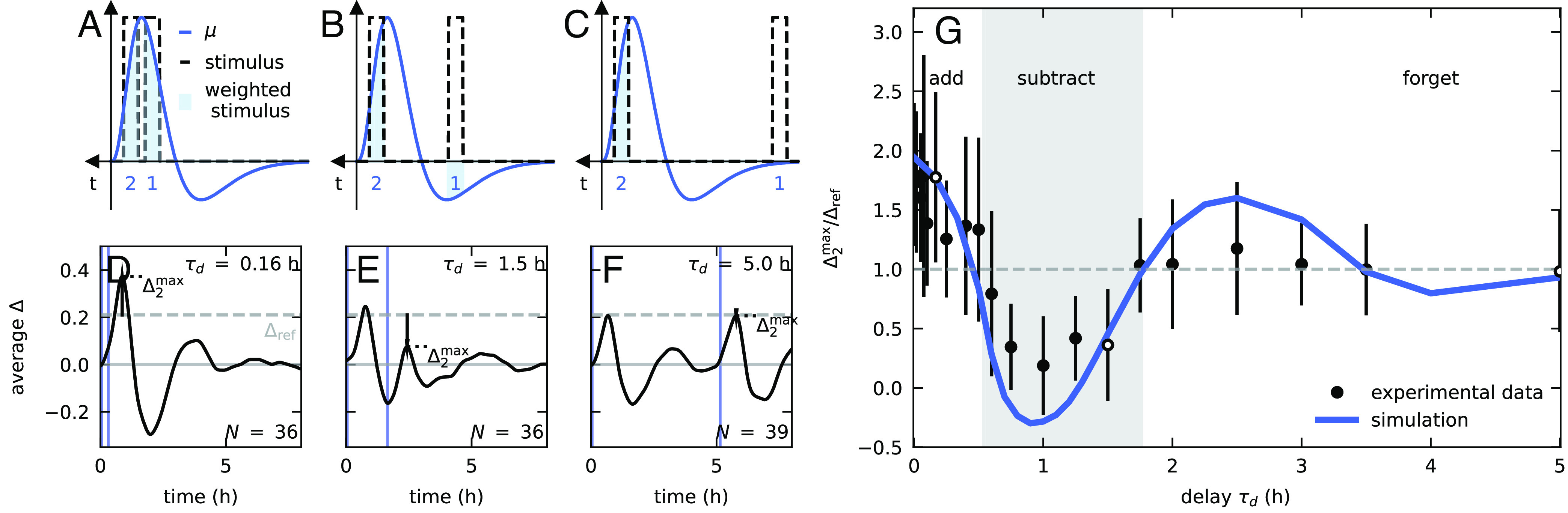
Model prediction and experimental observations of summation and subtraction regimes in two-stimulus experiments. (A–C) Graphical illustration of $\mu$ (blue line) compared to two stimuli (dashed bars) separated by different delay times ${\tau }_{\text{d}}$. Shadowed areas correspond to stimuli weighted by $\mu$. (A) For short ${\tau }_{\text{d}}$, both stimuli occur within first peak and are weighted positively. Coleoptiles are expected to respond to the weighted sum of stimuli, with a stronger response than for a single stimulus: verified in (D), the experimental response ${\mathrm{\Delta }}_2(t)$ for ${\tau }_{\text{d}}=10$ min (compare to ${\mu }_6$ in Fig. 1C). For reference, the dashed line represents ${\mathrm{\Delta }}_1^{\text{max}}$ for a single stimulus. (B) For intermediate ${\tau }_{\text{d}}$, the second stimulus occurs within the positive peak, weighted positively, and the first within the negative peak, weighted negatively. Coleoptiles expected to respond to weighted difference between stimuli, with a weaker response compared to a single stimulus: verified in (E), the response for ${\tau }_{\text{d}}=90$ min, roughly the time between the two peaks in ${\mu }_6$. (C) For ${\tau }_{\text{d}}$ larger than the timescale of $\mu$, the second stimulus occurs within the positive peak, weighted positively, while the second is multiplied by zero. The response is expected to be similar to that for a single stimulus: verified in (F), for ${\tau }_{\text{d}}=5$ h. (G) Maximal response of two-stimulus experiments relative to single stimulus ${\mathrm{\Delta }}_2^{\text{max}}/{\mathrm{\Delta }}_1^{\text{max}}$, for a range of ${\tau }_{\text{d}}$. Circles represent experimental data, and the blue line represents the simulated response based on the extracted kernel ${\mu }_6$. The shadowed area delineates the three regimes predicted in (A–C). The three white circles represent experiments (D–F).

We extended these two-stimulus experiments, in addition to simulations, for a range of values of ${\tau }_{\text{d}}$ between 0 and 5 h, spanning the timescale of ${\mu }_6$. In Fig. 4G, we report the values of the maximal response ${\mathrm{\Delta }}_2^{\text{max}}$ following the second stimulus, relative to ${\mathrm{\Delta }}_1^{\text{max}}$ as a reference, as a function of the delay time ${\tau }_{\text{d}}$, both for experiments and simulations. Our two-stimulus experiments, supported by simulations, reveal the three regimes we predicted earlier based on the form of the extracted memory kernel, illustrated in Fig. 4A–C: i) for short ${\tau }_{\text{d}}$ coleoptiles respond to the weighted sum of stimuli, in line with previous observations of temporal integration (12, 13, 25–29), and the response to the recent stimulus is stronger than for a single stimulus; ii) for ${\tau }_{\text{d}}$ of the order of the time between peaks, coleoptiles respond to the weighted difference of stimuli, and the response is weaker; and iii) for longer ${\tau }_{\text{d}}$, the coleoptiles respond to the recent stimulus alone. In SI Appendix, we show that these results are not an artifact of the relative orientation of the organs at the time of the second stimulus (SI Appendix, Fig. S3). Furthermore, while it is possible that proprioception may have a role in the observed memory, we note that it is a second-order response to the stimulus, mediated by the curvature. We also show that a neglected kernel in the proprioceptive term would not significantly affect the extracted gravitropic kernel for similar timescales (SI Appendix, Fig. S4).

Discussion

Together, these findings provide quantitative evidence that plants respond to the sum and difference of stimuli over different timescales, framed within a general mathematical framework. These computational processes can be identified as fundamental elements of natural search algorithms, common across diverse biological organisms (46). In the context of signal processing or control theory, the memory kernel may be interpreted as a band-pass filter. The summation of stimuli is effectively a moving average, improving the signal-to-noise ratio of an environmental signal. Subtraction of stimuli, which has never been reported before in plants, is required in order to compare signals over time, a strategy commonly used by a variety of living organisms in order to detect and climb signal gradients (47). For example, Segall et al. (33, 48) extracted a memory kernel describing the chemotactic response of bacteria to a chemical stimulus and found that it, too, was characterized by a positive peak followed by a negative one. On this basis, they found that bacteria compare chemical concentrations sampled over time, enabling them to identify chemical gradients.

Observed oscillations in the gravitropic reorientation of wheat coleoptiles have been conjectured to speed up the regulation of posture control (14, 49, 50). The half period of observed oscillations was found to be $1.1$ h (49, 50), consistent with the delay time ${\tau }_d$ of maximal subtraction, and anything occurring further than a full oscillation period ($2.2$ h) is forgotten (Fig. 4G). Within this context, our findings suggest that shoots may enhance regulation of posture control by comparing the relative inclination of the organ sensed at either side of an oscillation or circumnutation period, or equivalently detect a light gradient by comparing measured light intensities. Furthermore, as the ability of plants to integrate stimuli has been observed for a range of species and tropisms, it suggests that these computational abilities might be general.

Put together, our study provides the backdrop for understanding how plants may combine memory and movement in order to enhance movement control and sensing capabilities in the face of weak signals and fluctuating environments.

Materials and Methods

Wheat Growth Conditions.

Wheat coleoptiles were grown as described in refs. 45 and 13. Wild-type wheat seeds (Triticum aestivum cv. Ruta) were initially glued with floral glue to plastic boxes with draining holes at the bottom (germ pointing down). The boxes were filled with cotton and placed in a light-proof container, immersed in water. Coleoptiles were kept in a growth chamber at a temperature of 24 °C for 3 to 4 d. Coleoptiles were manipulated in darkness or dim green light to minimize exposure to actinic light.

Experimental Setup.

Our experimental apparatus consisted of an upright rotating platform holding 3D-printed casings each hosting a coleoptile box. A DC motor inclined the platform, and the inclination angle was measured and controlled with two optical fork sensors and a custom 3D-printed encoder wheel. During experiments images were taken every 1, 5, or 10 min, depending on the experiment, using a DSLR camera with a wide-angle lens, controlled by the Arduino. Pictures were taken with a dim green flash of 333 ms, placed perpendicular to the plane of motion. The setup was controlled by an Arduino microcontroller board running an in-house developed program. Each experiment started by placing upright coleoptile boxes on the rotating platform and waiting for an acclimation phase of 10 h in the dark. Coleoptiles were then gravistimulated by rotating the platform horizontally, ${\theta }_p=\pi /2$, during a stimulation time ${\tau }_{\text{s}}$, and then rotated back to the vertical position. We employed two types of protocols (schematically illustrated in Fig. 1B): i) single stimulus, for a range of ${\tau }_{\text{s}}$ values (in minutes: 1, 3, 5, 6, 12, 24, 35, 45, 60, 90 and 600), ii) double stimulus; apply two successive stimuli of ${\tau }_{\text{s}}=6\text{min}$ each, separated by a delay time ${\tau }_{\text{d}}$ (in minutes: 1, 3, 4.5, 6, 10, 15, 24, 30, 36, 45, 60, 75, 90, 105, 120, 150, 180, 210 and 240). The rotation of the platform takes $6$ s to tilt horizontally. Each experiment included at least 30 repetitions. Experiments were carried out over a range of times during the day, and any circadian contributions (51) are expected to be negligible.

Data Collection.

As described in Fig. 1A, the local frame of the rotating platform is $(\widehat{\mathbf{x}},\widehat{\mathbf{y}})$, where $\widehat{\mathbf{y}}$ is parallel to the upright position of coleoptiles. The angle of the stimulus ${\theta }_p$ is defined as the angle between the vertical of the platform and the direction of gravity, $cos{\theta }_p(t)=\widehat{\mathbf{g}}·\widehat{\mathbf{y}}(t)$. We extracted the center line of each coleoptile, for each image, using a version of the Python-based software Interekt (52). From the center line, we extracted the local angle $\theta (s,t)$ of the coleoptile with respect to $\widehat{\mathbf{y}}$, the apical and basal angles ${\theta }_{\text{tip}}(t)=\theta (L,t)$ and ${\theta }_{\text{base}}(t)=\theta (0,t)$, the total length $L(t)$, and the radius averaged over $s$, $R(t)$. The quantities ${\theta }_{\text{tip}}$ and ${\theta }_{\text{base}}$ were obtained by locally averaging $\theta (s)$ over 2 mm, i.e., less than $L_{\text{gz}}/10$, where $L_{\text{gz}}$ is the growth zone. This length scale also sets the minimum required size for a coleoptile to be included in our analysis, i.e., 4 mm. We also calculated ${\ell }_{\perp }(t)=\int \mathrm{d}ssin\left(\theta (s,t)-{\theta }_{\text{P}}(t)\right)$, the projection of the organ perpendicular to $\widehat{g}$. These quantities were further smoothed with a combination of a median filter and a lowpass filter to remove aberrant data points and allow the computation of smooth time derivatives.

Numerical Simulations.

We ran numerical simulations implementing a discretized version of Eq. 2. The code was written in Python and based on ref. 12, however allowing to implement any memory kernel or inclination protocol (including transient tilts or clinostat). Required parameters, such as $\mu (t)$, $\beta$, $\gamma$, $L$, and $\theta (s,t=0)$, were extracted from experiments (SI Appendix, Fig. S5).

Estimation of Gravitropic and Proprioceptive Gains β and γ.

The estimation of the $\beta$ and $\gamma$ was carried out from the permanent stimulation experiments. In order to compare the dynamics of the growing coleoptiles with our model and simulations, which do not take growth into account explicitly, we consider the normalized gravitropic response defined as $\mathrm{\Delta }(t)={\partial }_t\left({\theta }_{\text{tip}}-{\theta }_{\text{base}}\right)·R/v_{\mathrm{g}}$, where $R$ is the radius of the organ and $v_{\mathrm{g}}=dL/dt$ is the growth rate. The maximal value is termed the dimensionless gravitropic sensitivity ${\mathrm{\Delta }}^{\text{max}}\equiv \tilde{\beta }$ (45, 52, 53). In the limit of negligible growth, we have $\beta =R\tilde{\beta }/\dot{\epsilon }$ where $\dot{\epsilon }=v_{\text{g}}/L_{\text{gz}}$ is the average elongation rate of the plant organ and $L_{\text{gz}}$ the length of its growth zone (42). $\gamma$ is then extracted from the convergence length $L_{\text{c}}=\gamma /\beta$, found by fitting the steady-state angular profile $\theta (s)$ of each organ to an exponential (42): $\theta (s)=\mathrm{\Theta }\left(1-exp\left(-(s-s_0)/L_{\text{c}}\right)\right)+{\theta }_0$. For each plant, the fit was repeated and averaged over the last $100\text{min}$ of the experiment. When $s_0>0$, we can approximate $L_{\text{gz}}\approx L-s_0$. Extracted values are found in SI Appendix, Fig. S5.

Memory Kernel Estimation.

In the case of transient inclination, the gravitropic sensitivity $\beta$ is assumed constant, while the inclination angle ${\theta }_{\mathrm{P}}(t)$ is time-dependent. Integrating Eq. 2 over $s$, and assuming gravistimulation is zero for $t<0$, yields: $\left({\partial }_t+\gamma \right)\left({\theta }_{\text{tip}}(t)+{\theta }_{\text{base}}(t)\right)=-\beta {\int }_0^t\mu (t-t^{\prime }){\ell }_{\perp }(t^{\prime })\text{d}{t}^{\prime }$, where ${\ell }_{\perp }$ is the signed length of the organ projected on the axis normal to the stimulation direction. This can then be rewritten as a Volterra integral equation of the first kind on $\mu$ with ${\ell }_{\perp }$ as a kernel: $g(t)={\int }_0^t\mu (t^{\prime }){\ell }_{\perp }(t-t^{\prime })\text{d}{t}^{\prime }$, where $g=-1/\beta \left({\partial }_t+\gamma \right)\left({\theta }_{\text{tip}}+{\theta }_{\text{base}}\right)$. This integral equation is then solved in the classical way by first turning it into a Volterra integral of the second kind by differentiating it with respect to time and then discretizing it (54). The initial value is ${\mu }_0={\dot{g}}_0/{\ell }_0^{\perp }$, and the solution is then built by successive iterations, for each i: ${\mu }_i=({\dot{g}}_i-\mathrm{\Delta }t\sum _{k=0}^{i-1}{\mu }_k{\dot{\ell }}_{i-k}^{\perp })/({\ell }_0^{\perp }+{\dot{\ell }}_0^{\perp }\mathrm{\Delta }t)$. In the case of finite stimuli ${\tau }_{\text{s}}$, we approximate the sharp transitions of ${\theta }_{\text{P}}$ with a sigmoid curve with characteristic time $\mathrm{\Delta }t=1$min. We have successfully tested this algorithm on a set of Volterra integral equations of the first kind where an analytical solution was known (55, 56). We validated the described method for our model in Eq. 2. We ran simulations for transient inclinations of duration ${\tau }_{\text{s}}$ with arbitrarily chosen memory kernels ${\mu }_{\mathrm{in}}$. From the simulated dynamics, memory kernels were estimated using the method described here and were found to be consistent with the original, regardless of the shape of the kernel or the stimulus duration ${\tau }_{\text{s}}$ (SI Appendix, Fig. S6). Extracting of memory kernel from experimental data: For each coleoptile, we extracted $\mu (t)$ from the trajectory ${\theta }_{\text{tip}}(t)$. We discarded instances where the algorithm diverged. We then averaged over repetitions resulting in an average $\mu$. We do not take an explicit account of growth when estimating of $\mu$, and to the first approximation, we neglect the possible slow drift of ${\ell }_{\perp }$ due to growth.

Supplementary Material

Appendix 01 (PDF)

Data, Materials, and Software Availability

Python code and processed experimental measurements data have been deposited in Zenodo (http://dx.doi.org/10.5281/zenodo.8191754) (57).

References

- 1.Cahill J. F. Jr., et al. , Plants integrate information about nutrients and neighbors. Science 328, 1657 (2010). [DOI] [PubMed] [Google Scholar]
- 2.Dener E., Kacelnik A., Shemesh H., Pea plants show risk sensitivity. Curr. Biol. 26, 1763–1767 (2016). [DOI] [PubMed] [Google Scholar]
- 3.Hodge A., Root decisions. Plant Cell Environ. 32, 628–640 (2009). [DOI] [PubMed] [Google Scholar]
- 4.Paul A. L., Amalfitano C. E., Ferl R. J., Plant growth strategies are remodeled by spaceflight. BMC Plant Biol. 12, 232 (2012). [DOI] [PMC free article] [PubMed] [Google Scholar]
- 5.Ciszak M., Masi E., Baluška F., Mancuso S., Plant shoots exhibit synchronized oscillatory motions. Commun. Integr. Biol. 9, e1238117 (2016). [DOI] [PMC free article] [PubMed] [Google Scholar]
- 6.Faget M., et al. , Root-root interactions: Extending our perspective to be more inclusive of the range of theories in ecology and agriculture using in-vivo analyses. Ann. Bot. 112, 253–266 (2013). [DOI] [PMC free article] [PubMed] [Google Scholar]
- 7.Pereira M. L., Sadras V. O., Batista W., Casal J. J., Hall A. J., Light-mediated self-organization of sunflower stands increases oil yield in the field. Proc. Natl. Acad. Sci. U.S.A. 114, 7975–7980 (2017). [DOI] [PMC free article] [PubMed] [Google Scholar]
- 8.Paya A. M., Silverberg J. L., Padgett J., Bauerle T. L., X-ray computed tomography uncovers root-root interactions: Quantifying spatial relationships between interacting root systems in three dimensions. Front. Plant Sci. 6 (2015). 10.3389/fpls.2015.00274. [DOI] [PMC free article] [PubMed]
- 9.Gruntman M., Groß D., Májeková M., Tielbörger K., Decision-making in plants under competition. Nat. Commun. 8, 2235 (2017). [DOI] [PMC free article] [PubMed] [Google Scholar]
- 10.McCleery W. T., Mohd-Radzman N. A., Grieneisen V. A., Root branching plasticity: Collective decision-making results from local and global signalling. Curr. Opin. Cell Biol. 44, 51–58 (2017). [DOI] [PubMed] [Google Scholar]
- 11.Karban R., Orrock J. L., A judgment and decision making model for plant behavior. Ecology 99, 1909–1919 (2018). [DOI] [PubMed] [Google Scholar]
- 12.Meroz Y., Bastien R., Mahadevan L., Spatio-temporal integration in plant tropisms. J. R. Soc. Interface 16, 20190038 (2019). [DOI] [PMC free article] [PubMed] [Google Scholar]
- 13.Chauvet H., Moulia B., Legué V., Forterre Y., Pouliquen O., Revealing the hierarchy of processes and time-scales that control the tropic response of shoots to gravi-stimulations. J. Exp. Botany 70, 1955–1967 (2019). [DOI] [PMC free article] [PubMed] [Google Scholar]
- 14.Moulia B., Douady S., Hamant O., Fluctuations shape plants through proprioception. Science 372, eabc6868 (2021). [DOI] [PubMed] [Google Scholar]
- 15.Fromm H., Root plasticity in the pursuit of water. Plants 8, 236 (2019). [DOI] [PMC free article] [PubMed] [Google Scholar]
- 16.Moulia B., Badel E., Bastien R., Duchemin L., Eloy C., The shaping of plant axes and crowns through tropisms and elasticity: An example of morphogenetic plasticity beyond the shoot apical meristem. New Phytol. 233, 2354–2379 (2022). [DOI] [PubMed] [Google Scholar]
- 17.Bastien R., Meroz Y., The kinematics of plant nutation reveals a simple relation between curvature and the orientation of differential growth. PLoS Comput. Biol. 12, e1005238 (2016). [DOI] [PMC free article] [PubMed] [Google Scholar]
- 18.van Schijndel L., Snoek B. L., ten Tusscher K., Embodiment in distributed information processing: “solid’’ plants versus “liquid’’ ant colonies. Quant. Plant Biol. 3, e27 (2022). [DOI] [PMC free article] [PubMed] [Google Scholar]
- 19.Moulton D. E., Oliveri H., Goriely A., Multiscale integration of environmental stimuli in plant tropism produces complex behaviors. Proc. Natl. Acad. Sci. U.S.A. 117, 32226–32237 (2020). [DOI] [PMC free article] [PubMed] [Google Scholar]
- 20.Meroz Y., Plant tropisms as a window on plant computational processes. New Phytol. 229, 1911–1916 (2021). [DOI] [PubMed] [Google Scholar]
- 21.Duran-Nebreda S., Bassel G. W., Plant behaviour in response to the environment: Information processing in the solid state. Philos. Trans. R. Soc. B 374, 20180370 (2019). [DOI] [PMC free article] [PubMed] [Google Scholar]
- 22.Bassel G. W., Information processing and distributed computation in plant organs. Trends Plant Sci. 23, 994–1005 (2018). [DOI] [PubMed] [Google Scholar]
- 23.Fitting H., Untersuchungen ÃŒber den geotropischen reizvorgang. Teil i. Die geotropische empfindlichkeit der pflanzen. teil ii. weitere erfolge mit der intermittierenden reizung. Jahrb. Wiss. Bot. 41 (221–330), 331–398 (1905). [Google Scholar]
- 24.Nathansohn A., Pringseheim E., Uber die summation intermittierren der lichtreize. Jahrb. Wiss. Bot. 45, 137–190 (1908). [Google Scholar]
- 25.Volkmann D., Tewinkel M., Gravisensitivity of cress roots: Investigations of threshold values under specific conditions of sensor physiology in microgravity. Plant Cell Environ. 19, 1195–1202 (1996). [DOI] [PubMed] [Google Scholar]
- 26.Pickard B. G., Geotropic response patterns of the avenacoleoptile. I. Dependence on angle and duration of stimulation. Cana. J. Bot. 51, 1003–1021 (1973). [Google Scholar]
- 27.Kataoka H., Phototropic responses of vaucheria geminata to intermittent blue light stimuli. Plant Physiol. 63, 1107–1110 (1979). [DOI] [PMC free article] [PubMed] [Google Scholar]
- 28.Briggs W. R., Light dosage and phototropic responses of corn and oat coleoptiles. Plant Physiol. 35, 951–962 (1960). [DOI] [PMC free article] [PubMed] [Google Scholar]
- 29.Johnsson A., Karlsson C., Iversen T. H., Chapman D. K., Random root movements in weightlessness. Physiol. Plant. 96, 169–178 (1996). [PubMed] [Google Scholar]
- 30.D. Des Cloizeaux, “Linear response, generalized susceptibility and dispersion theorya” in Theory of Condensed Matter. Lectures Presented at an International Course, F. Bassani, G. Caglioti, J. Ziman, Eds. (International Atomic Energy Agency, Vienna, 1968).
- 31.Cowan N. J., et al. , Feedback control as a framework for understanding tradeoffs in biology. Integr. Comp. Biol. 54, 223–237 (2014). [DOI] [PubMed] [Google Scholar]
- 32.Block S. M., Segall J. E., Berg H. C., Impulse responses in bacterial chemotaxis. Cell 31, 215–226 (1982). [DOI] [PubMed] [Google Scholar]
- 33.Segall J. E., Block S. M., Berg H. C., Temporal comparisons in bacterial chemotaxis. Proc. Natl. Acad. Sci. U.S.A. 83, 8987–8991 (1986). [DOI] [PMC free article] [PubMed] [Google Scholar]
- 34.Lipson E. D., White noise analysis of phycomyces light growth response system. I. Normal intensity range. Biophysi. J. 15, 989 (1975). [DOI] [PMC free article] [PubMed] [Google Scholar]
- 35.Prentice-Mott H. V., et al. , Directional memory arises from long-lived cytoskeletal asymmetries in polarized chemotactic cells. Proc. Natl. Acad. Sci. U.S.A. 113, 1267–1272 (2016). [DOI] [PMC free article] [PubMed] [Google Scholar]
- 36.Kaspar C., Ravoo B., van der Wiel W. G., Wegner S., Pernice W., The rise of intelligent matter. Nature 594, 345–355 (2021). [DOI] [PubMed] [Google Scholar]
- 37.Peak D., West J. D., Messinger S. M., Mott K. A., Evidence for complex, collective dynamics and emergent, distributed computation in plants. Proc. Natl. Acad. Sci. U.S.A. 101, 918–922 (2004). [DOI] [PMC free article] [PubMed] [Google Scholar]
- 38.Keim N. C., Paulsen J. D., Zeravcic Z., Sastry S., Nagel S. R., Memory formation in matter. Rev. Mod. Phys. 91, 035002 (2019). [Google Scholar]
- 39.Bhattacharyya K., Zwicker D., Alim K., Memory formation in adaptive networks. Phys. Rev. Lett. 129, 028101 (2022). [DOI] [PubMed] [Google Scholar]
- 40.Sachs J., Über orthotrope und plagiotrope pflanzentheile. Arb. Bot. Inst. Wurzburg 2, 226–284 (1882). [Google Scholar]
- 41.Moulia B., Fournier M., The power and control of gravitropic movements in plants: A biomechanical and systems biology view. J. Exp. Bot. 60, 461–486 (2009). [DOI] [PubMed] [Google Scholar]
- 42.Bastien R., Bohr T., Moulia B., Douady S., Unifying model of shoot gravitropism reveals proprioception as a central feature of posture control in plants. Proc. Natl. Acad. Sci. U.S.A. 110, 755–760 (2013). [DOI] [PMC free article] [PubMed] [Google Scholar]
- 43.Levernier N., Pouliquen O., Forterre Y., An integrative model of plant gravitropism linking statoliths position and auxin transport. Front. Plant Sci. 12, 474 (2021). [DOI] [PMC free article] [PubMed] [Google Scholar]
- 44.Nakamura M., Nishimura T., Morita M. T., Gravity sensing and signal conversion in plant gravitropism. J. Exp. Bot. 70, 3495–3506 (2019). [DOI] [PubMed] [Google Scholar]
- 45.Chauvet H., Pouliquen O., Forterre Y., Legué V., Moulia B., Inclination not force is sensed by plants during shoot gravitropism. Sci. Rep. 6, 1–8 (2016). [DOI] [PMC free article] [PubMed] [Google Scholar]
- 46.Hein A. M., Carrara F., Brumley D. R., Stocker R., Levin S. A., Natural search algorithms as a bridge between organisms, evolution, and ecology. Proc. Natl. Acad. Sci. U.S.A. 113, 9413–9420 (2016). [DOI] [PMC free article] [PubMed] [Google Scholar]
- 47.Nelson M. E., MacIver M. A., Sensory acquisition in active sensing systems. J. Compa. Physiol. A 192, 573–586 (2006). [DOI] [PubMed] [Google Scholar]
- 48.Berg H. C., E. coli in Motion (Springer, New York, 2004). [Google Scholar]
- 49.Tarui Y., Iino M., Gravitropism of oat and wheat coleoptiles: Dependence on the Stimulation angle and involvement of autotropic straightening. Plant Cell Physiol. 38, 1346–1353 (1997). [DOI] [PubMed] [Google Scholar]
- 50.Bastien R., Guayasamin O., Douady S., Moulia B., Coupled ultradian growth and curvature oscillations during gravitropic movement in disturbed wheat coleoptiles. PLoS One 13, 1–16 (2018). [DOI] [PMC free article] [PubMed] [Google Scholar]
- 51.Tolsma J., et al. , The circadian-clock regulates the gravitropic response. Gravit. Space Res. 9, 171–186 (2021). [Google Scholar]
- 52.F. P. Hartmann et al., “Methods for a quantitative comparison of gravitropism and posture control over a wide range of herbaceous and woody species” in Plant Gravitropism (Springer, 2022), pp. 117–131. [DOI] [PubMed]
- 53.Bastien R., Douady S., Moulia B., A unifying modeling of plant shoot gravitropism with an explicit account of the effects of growth. Front. Plant Sci. 5, 136 (2014). [DOI] [PMC free article] [PubMed] [Google Scholar]
- 54.Press W. H., Teukolsky S. A., Vetterling W. T., Flannery B. P., Numerical Recipes 3rd Edition: The Art of Scientific Computing (Cambridge University Press, 2007). [Google Scholar]
- 55.Linz P., Numerical methods for volterra integral equations of the first kind. Comput. J. 12, 393–397 (1969). [Google Scholar]
- 56.Babolian E., Masouri Z., Direct method to solve volterra integral equation of the first kind using operational matrix with block-pulse functions. J. Comput. Appl. Math. 220, 51–57 (2008). [Google Scholar]
- 57.M. Rivière, Y. Meroz, Data and code for: Plants sum and subtract stimuli over different timescales. Zenodo. 10.5281/zenodo.8191754. Deposited 28 July 2023. [DOI] [PMC free article] [PubMed]
Associated Data
This section collects any data citations, data availability statements, or supplementary materials included in this article.
Supplementary Materials