Targeted deep learning classification and feature extraction for clinical diagnosis

Summary

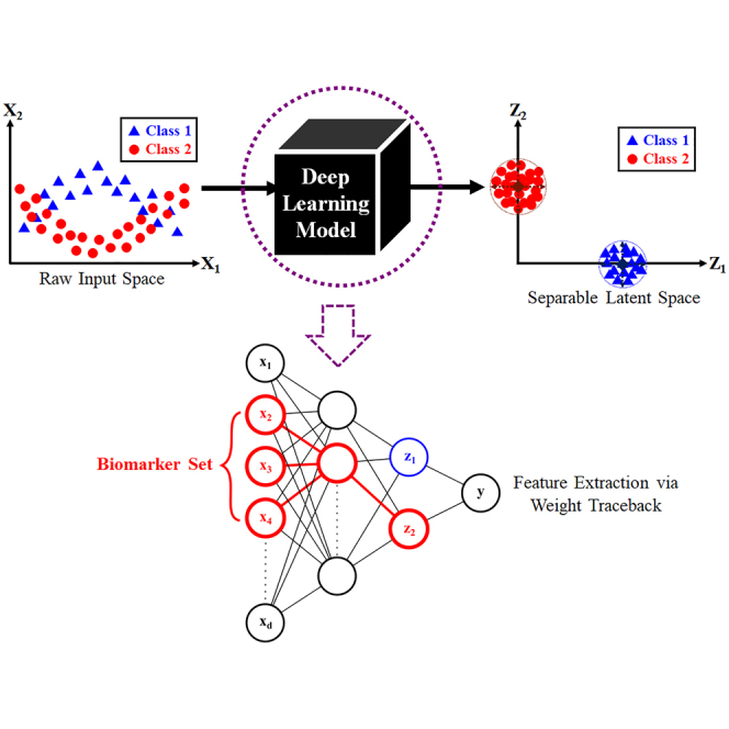
Protein biomarkers can be used to characterize symptom classes, which describe the metabolic or immunodeficient state of patients during the progression of a specific disease. Recent literature has shown that machine learning methods can complement traditional clinical methods in identifying biomarkers. However, many machine learning frameworks only apply narrowly to a specific archetype or subset of diseases. In this paper, we propose a feature extractor which can discover protein biomarkers for a wide variety of classification problems. The feature extractor uses a special type of deep learning model, which discovers a latent space that allows for optimal class separation and enhanced class cluster identity. The extracted biomarkers can then be used to train highly accurate supervised learning models. We apply our methods to a dataset involving COVID-19 patients and another involving scleroderma patients, to demonstrate improved class separation and reduced false discovery rates compared to results obtained using traditional models.

Graphical abstract

Highlights

• •Machine learning and feature extraction
• •Deep learning classifier
• •Protein biomarker and signature discovery

Health sciences; Computer-aided diagnosis method; Artificial intelligence applications

Introduction

Background

Machine learning (ML) is a powerful, emerging modeling approach which can potentially complement traditional clinical tasks, such as disease diagnosis,¹ protein biomarker identification,^2,3,4 and drug discovery.⁵ Despite the abundance of ML-related literature, there is currently a lack of unified framework in deep learning (DL)⁶ models, with respect to these clinical tasks. In this article, we propose a DL-based workflow which accomplishes the following. Given a raw dataset containing N patient samples, d raw variables, and C known conditions or symptom classes, the main objectives are to accurately predict the class membership for each patient, as well as discover key signatures or biomarkers characterizing each class.

The high-dimensional nature of many clinical datasets is addressed by two main families of ML models. The first family consists of Dimensionality reduction (DR) algorithms, which include principal component analysis (PCA),^7,8 multi-dimensional scaling (MDS),⁹ t-distributed stochastic neighbor embedding (t-SNE),¹⁰ uniform manifold approximation and projection (UMAP),¹¹ locally linear embedding (LLE),¹² and isometric mapping (ISOMAP).¹³ The second family consists of Feature Engineering models, such as Feature Selectors,^{14,15,16,17,18,19} Feature Extractors,^{20,21,22,23,24,25} and kernel basis-function methods.^26,27 Both ML families are used as a precursor to classification problems, in hope of discovering a latent space with clearly distinguishable class clusters. However, due to the nuances present in any given dataset, the analyst may exhaust all traditional options and still fail to obtain a class-separable latent space. To address this problem, we propose the use of DL⁶ models to actively seek out a class-separable latent projection. DL models are not constrained by the type of underlying data structure, as they are universal function approximators²⁸ which can closely estimate any non-linearity by sheer brute-force combination of activation units. Moreover, DL models are Supervised Learning in nature, which means they can utilize any information available in the outcome labels to guide the discovery of a class-separable latent space. Since traditional DL objective functions focus on minimizing prediction error, we enhance class cluster identity by including an additional discriminative center-loss (DCL) term, an adaptation of the original idea in Wen et al.²⁹ The DCL term penalizes widely spread or loose clusters, and therefore the discovered latent spaces are guaranteed to carry the most tightly-knit clusters possible. This in turn leads to significantly increased prediction accuracies, as well as the ability to perform meaningful feature extraction.

The specific objectives of our work are as follows. First, we show that the proposed discriminative center-loss deep learning (DCLDL) model discovers class clusters that are more well-defined, compared to those discovered by traditional DR algorithms. Moreover, we also show that meaningful features can be extracted from the DCLDL-discovered latent space, which manifest as protein biomarker sets associated with each patient class. From a clinical perspective, the main contributions of our work include the significant reduction of false diagnosis rates, as well as a means of discovering influential biomarkers which may be used to guide subsequent precision treatment. The overall workflow can be seen in Figure 1. In each case study, we highlight the strengths of our methodology by comparing the predictive diagnosis and feature map results obtained across a wide variety of ML algorithms (Figure 2). We demonstrate the efficacy of our approach through 4 case studies, starting with a proof-of-concept using the IRIS³⁰ and MNIST³¹ benchmark datasets. This is followed by the analysis of two clinical datasets concerning real patients, related to the COVID-19³ and scleroderma diseases (Figure 3).

Figure 1.

Proof-of-concept workflow for our proposed ML approach

Figure 2.

Detailed ML workflow for the Scleroderma patient dataset

Figure 3.

Proteomic sample acquisition and analysis workflow for the Scleroderma patients

Results and discussion

Benchmark datasets

We begin by demonstrating the predictive and feature extraction capabilities of the proposed algorithm on two well-known ML benchmarks. The first is the Fisher IRIS dataset,³⁰ and the second is the Modified National Institute of Standards and Technology (MNIST) digits dataset.³¹ These benchmarks represent classification problems which are straightforward in nature, with data classes that are easily distinguishable by any competent model. This is evidenced by many highly accurate models that already exist in literature, such as DL models with sub-$1\%$ error rates.^32,33,34 Hence, our goal with these benchmarks is to pick a baseline DL model with sufficient accuracy, and show that the integration of the DCLDL loss (Equation 9) results in improved class-specific accuracies as well as the correct identification of relevant features or feature maps. Conversely, if the DCLDL integration cannot provide any improvement in classification accuracy for these baselines, then there is no point considering DCLDL for more complicated scenarios.

IRIS benchmark

The first benchmark is the Fisher IRIS dataset³⁰ which contains $N=150$ total flower samples. The samples are distributed evenly into $C=3$ flower classes (Setosa - Class 0, Versicolor - Class 1, and Virginica - Class 2), with 50 samples belonging to each class. The $d=4$ raw variables describing each flower are sepal length, sepal width, petal length, and petal width. In our demonstration, we construct a baseline ANN model, then insert the DCLDL term (Equation 9) into the existing loss function and observe any resulting effects on class prediction accuracy. We intentionally train a baseline model with slightly sub-$100\%$ accuracy, so that there would be room for the DCLDL loss to improve upon. Both models are 2-layer fully connected ANNs, with 8 neurons in the first hidden layer and $C=3$ neurons in the second and last hidden layer. We use a learning rate of $\alpha =5\cdot {10}^{-3}$ and regularizer (weight decay) of $5\cdot {10}^{-2}$ for both models. For the DCLDL-included model, we use a center-binding strength of $\lambda =2.5\cdot {10}^{-1}$ to tighten the spread of each class cluster. In order to place the two models on equal footing for subsequent comparison, we randomly select training and testing samples, but use the same selected samples to evaluate performance for both models. We train both models over 1000 epochs, whilst ensuring that each loss reaches an acceptably low number. After the DCLDL-included model is sufficiently-trained, we perform feature extraction using weight traceback to determine the most important features that distinguish the 3 flower classes.

The results from this benchmark study are as follows. First, the class-specific accuracies summarized in Table 1 show that we achieve perfect ($100\%$) training and testing accuracy for the Setosa (Class 0) and Virginica (Class 2) flowers. The only misclassified class is that of Versicolor (Class 1), which has $95\%$ training accuracy and $80\%$ testing accuracy in the baseline model. The addition of the DCLDL loss results in a significant improvement to both model training and generalization, specifically a $2.5\%$ increase in training accuracy and a $10\%$ increase in testing accuracy. In both models, the misclassified Versicolor (Class 1) flowers are falsely identified as Virginica (Class 2) flowers, as shown in Figure 4. Neither model has trouble distinguishing Setosa (Class 0) from the remaining two classes, as evidenced by the Setosa class cluster being comfortably distanced from the others. Moreover, notice that the spread of the class clusters is reduced by the addition of the DCLDL loss, as originally expected. Finally, both models show difficulty distinguishing between Versicolor (Class 1) and Virginica (Class 2) flowers, as indicated by the slight overlap between the two class clusters. The DCLDL-included model reduces the overlap by tightening the class clusters, which results in an improved classification accuracy for the Versicolor (Class 1) flowers (Table 1).

Table 1.

Performance comparison between ANN models, with and without the DCLDL loss, on the IRIS dataset

Class	ANN		ANN $+$ DCLDL
	Train Acc $(\%)$	Test Acc $(\%)$	Train Acc $(\%)$	Test Acc $(\%)$
0 (Setosa)	100.0	100.0	100.0	100.0
1 (Versicolor)	95.0	80.0	97.5	90.0
2 (Virginica)	100.0	100.0	100.0	100.0

Figure 4.

The distribution of class clusters in the last hidden layer of each ANN model

The DCLDL-included model is not only capable of improving class-specific accuracy, but is also capable of identifying the correct important features. According to existing domain knowledge regarding the IRIS flowers,³⁰ petal length and petal width are the key decisive features distinguishing the classes apart. On the other hand, sepal width and sepal length are much less consequential. This expected result is reflected in the following Figure 5, which show significantly larger feature weights for petal length and petal width than those for sepal width and sepal length. Since petal length has a wider numerical range of $1.0\sim 6.9cm$ compared to petal width with a range of $0.1\sim 2.5cm$, it makes sense that petal length has much larger feature weights compared to petal width. Moreover, the key feature distinguishing Setosa flowers from the rest is a petal length of $<1.9cm$. This explains why petal length appears as the most important feature for the Setosa class in Figure 5, as well as the heavy negative correlation. As for the remaining two classes, the data shows that Versicolor flowers typically have a of petal length between $3.0cm$ and $5.1cm$, and a petal width between $1.0cm$ and $1.8cm$. On the other hand, the majority of Virginica flowers are characterized by a petal length of $>5.1cm$, with only a small remainder of them having a petal length between $4.5cm$ and $5.1cm$. The petal width of Virginica flowers ranges between $1.4cm$ and $2.5cm$. The overlaps in petal length and petal width ranges between Versicolor and Virginica flowers explains why the classifiers have a difficult time separating these two classes. Moreover, in Figure 5, the positive weights for Versicolor flowers reflect the distinction between Versicolor and Setosa flowers, which are smaller in petal length and petal width. Similarly, the negative weights reflect the distinction between Versicolor and Virginica flowers, which are larger in petal length and petal width. The majority of Versicolor flowers are characterized by lower values of petal length, followed by lower values of petal width; this explains why they are more negatively-correlated with petal length and petal width rather than positively-correlated. Specifically, Versicolor flowers only need a condition of petal length $>1.9cm$ to be distinguished from Setosa flowers, whilst requiring a more nuanced set of conditions to be separated from Virginica flowers.

Figure 5.

Ranked importance of each flower feature, determined by weight-traceback feature extraction

MNIST benchmark

The second benchmark is the MNIST dataset,³¹ which contains $N=70000$ grayscale handwritten images of the ten numerical digits 0 through 9. Each image is a 2-dimensional square of 28 pixel rows and 28 pixel columns. The total $N=70000$ images are divided into pre-specified sets of $N_{train}=60000$ training images and $N_{test}=10000$ testing images. For this benchmark study, we selected the LeNet-5 Convolutional Neural Network (CNN)³⁵ as the baseline, due to its widespread acceptance as a high-performance classifier. After this baseline model is established, we add the DCLDL term (Equation 9) to its existing loss function, and observe any effects on class prediction accuracy and feature map clarity. Both CNN models are trained using a total of 300 epochs, whilst ensuring that the training loss has settled around an acceptably low value. Both models use a regularizer (weight decay) of $1\cdot {10}^{-2}$ and a learning rate of $\alpha =1\cdot {10}^{-2}$. Finally, the DCLDL-included model uses a center-binding strength of $\lambda =5\cdot {10}^{-4}$ to tighten the spread of each class cluster.

The results of this benchmark study are as follows. First, Table 2 shows that the traditional LeNet-5 CNN is able to achieve $>90\%$ training and testing accuracy for 8 out of the 10 numerical digits. However, it struggles to correctly classify the digits 5 ($89.6\%$ training accuracy, $88.3\%$ testing accuracy) and 9 ($86.4\%$ training accuracy, $87.5\%$ testing accuracy). This is reflected in the cluster distributions in Figure 6, which shows a dispersed digit 9 cluster that overlaps extensively with other digits. Many digit 9 images are confused with digit 7 and digit 4 clusters, and this makes sense intuitively due to the similarity in shape between these three digits. Moreover, the extent of overlap between the training set clusters is higher than those between the testing set clusters. The higher testing set accuracies in Table 2 reflect this point. Table 2 also shows a performance improvement in all digits due to the inclusion of the DCLDL loss, except for the digit 4 ($0.3\%$ drop in training accuracy and $1\%$ drop in testing accuracy). The DCLDL loss tightens the spread of each class cluster, thereby reducing inter-cluster overlap. The digits 5 and 9, which the baseline LeNet-5 CNN struggled with, saw the largest improvements. Specifically, the training accuracy of digit 5 images improved by $8.1\%$, and the testing accuracy by $9.1\%$. Similarly, the training accuracy of digit 9 images improved by $9.6\%$, and the testing accuracy by $8.5\%$.

Table 2.

Performance comparison between two LeNet-5 models, with and without the DCLDL loss, on the MNIST digits dataset

Digit	LeNet-5		LeNet-5 $+$ DCLDL
	Train Acc $(\%)$	Test Acc $(\%)$	Train Acc $(\%)$	Test Acc $(\%)$
0	98.4	98.8	99.1	99.2
1	97.7	99.1	98.4	99.2
2	94.4	95.1	98.3	98.5
3	91.7	93.4	97.3	98.2
4	98.0	98.1	97.7	97.1
5	89.6	88.3	97.7	97.4
6	98.0	97.2	98.4	97.8
7	95.0	93.2	97.8	96.7
8	92.5	93.7	93.3	94.6
9	86.4	87.5	96.0	96.0

Figure 6.

The distribution of digit image clusters in the last hidden layer of each LeNet-5 model, visualized in 2-D space by means of t-SNE compression

Biological datasets

COVID-19 dataset

In this demonstration, we apply our proposed DL model to a pre-existing COVID-19 patient dataset, which can be found in the original publication by Shu et al.³ We focus our analysis on the first patient cohort, which contains $N=62$ total patient samples and abundance counts from 865 protein types. The patients fall into $C=4$ symptom categories, which consist of 8 Healthy (Class 0) samples, 20 Mild (Class 1) samples, 14 Severe (Class 2) samples, and 20 Fatal (Class 3) samples. In terms of data pre-processing, we first removed any protein with zero abundance in more than $70\%$ of all patients, a step which was also performed by Shu et al.³ This resulted in $d=530$ remaining non-sparse proteins. We then normalized all remaining protein abundance counts to a value range between 0 and 1. The preprocessed data is then compressed using the traditional DR algorithms of PCA, MDS, ISOMAP, LLE, and UMAP. We also perform compression using two DL models: a traditional one without the DCL component, and our proposed DCLDL model. The DCLDL network (Figure 7) has 2 hidden layers, and $k^{\left[1\right]}=45$ neurons in its first layer. This number is chosen such that the dimensionality is compressed by a factor of approximately 11 in each layer.

Figure 7.

DCLDL model used to analyze the patients from the COVID-19 dataset

The latent spaces discovered by traditional DR techniques are shown in the following Figures 8A through 8E. Although LLE and UMAP appear to be the most successful in discovering class-separable latent spaces, overlap still exists between the Severe and Fatal class clusters. The latent spaces discovered by the remaining methods of PCA, MDS, and ISOMAP yield weakly-identifiable class clusters with high extents of overlap. The only redeeming result is the fact that the Healthy patient cluster appears to be safely distanced from all remaining class clusters. This implies a fundamental difference in the underlying data structure of the Healthy class, compared to all other classes. When we compare and contrast the feature maps discovered by two DL models (Figures 8F and 8G), the largest improvement can be visualized as the significantly increased distances between class clusters. The clusters in the DCLDL feature map are safely distanced apart, which means false diagnosis is almost impossible. On the other hand, the cluster overlaps in the other feature maps imply potential risks of false discoveries.

Figure 8.

Comparison of feature maps discovered by various ML algorithms

We now show that the clearly-separated class clusters in the DCLDL feature map (Figure 8G) have improved the accuracy of patient classification. We use every feature map in Figure 8 to train Supervised Learning classifiers, and compare the prediction accuracy of all 4 patient classes. We select Random Forests (RFs) and Support Vector Machines (SVMs) as the classifiers, training them using $80\%$ of the available patient samples, and testing on the remaining $20\%$. A total of 100 RF and SVM models are trained; every run uses different, randomly-selected sets of training and testing samples. The final model accuracy for each model type is expressed as an ensemble average taken across all 100 models. The overall RF and SVM model accuracies are reported in Figure 9. Note that these plots do not show the specific accuracies achieved by the models for each patient class. To elucidate these class-specific accuracies, we report the test set performances averaged across 100 runs, in form of confusion matrices in Figures 10 and 11. Note that we make a comparison to the base-case scenario, in which all $d=530$ proteins are used as inputs. In the base-case scenario, RF models were able to diagnose Healthy and Mild patient classes with zero false discoveries. For the remaining classes, RF models correctly diagnosed $77\%$ of all Severe patients, with the remaining $23\%$ misdiagnosed as Fatal patients. RF models also correctly diagnosed $98\%$ of all Fatal patients, with the remaining $2\%$ misdiagnosed as Severe patients. On the other hand, the SVM models performed poorly overall. In the base-case scenario, SVMs completely misdiagnosed the Healthy patient class, mistaking $90\%$ of them as Mild patients and $10\%$ as Fatal patients. SVMs also completely missed Severe patients, misdiagnosing $88\%$ of them as Fatal and $12\%$ of them as Mild. Although SVM performance was better for Mild ($98\%$ accuracy) and Fatal patients ($96\%$), its overall diagnosis accuracy is still low. When the feature maps from LLE and UMAP are used, some visible but inconsistent accuracy improvements are observed. For instance, by using UMAP latent features (Figure 10G), RF models were able to diagnose Severe patients with $89\%$ accuracy vs. $77\%$ in base case, whereas the performance degraded for Mild and Fatal patients. By using LLE latent features (Figure 11F), SVM models were able to perfectly diagnose Healthy, Mild, and Fatal patients, with $27\%$ of Severe patients being misdiagnosed. When the biomarkers discovered by Shu et al.³ are used for Supervised Learning, performance is similar or improved compared to baseline (Figures 10H and 11H). However, the 4 patient classes still remain confounded with significant false discovery rates. Finally, when the DCLDL latent features are used for diagnosis, perfect classification is possible with zero false discoveries (Figures 10I and 11I). This result is unsurprising, as the class clusters in Figure 8G are clearly separated from one another, thereby allowing even linear classifiers to easily identify separating boundaries.

Figure 9.

RF and SVM model accuracies obtained by training on the COVID-19 dataset

The bars represent average accuracy across 100 runs, while the vertical error bars represent maximum and minimum accuracies.

Figure 10.

RF model testing accuracy with respect to each of the 4 patient classes, averaged across 100 runs

Figure 11.

SVM model testing accuracy with respect to each of the 4 patient classes, averaged across 100 runs

We now analyze the protein biomarkers identified by performing weight traceback on the DCLDL model, and compare them with the biomarkers identified by Shu et al.³ Our method extracted a decisive biomarker set consisting of [LILRA2, IGLV5-39, CCDC158, MCAM], in terms of overall diagnosis. On the other hand, Shu et al.³ identified [CETP, FETUB] as the main biomarkers for overall diagnosis. The two sets of biomarkers are obviously inconsistent; however, our biomarkers allow perfect diagnosis of each patient class (Figures 10I and 11I), whereas the biomarkers extracted by Shu et al.³ lead to misclassifications (Figures 10H and 11H). This result strengthens the argument that from a pure predictive standpoint, biomarkers identified using ML may outperform those discovered by traditional assays. In Table 3, we report the top biomarkers that distinguish Mild patients from Severe patients. Although many of them are again inconsistent with the biomarkers identified by Shu et al.,³ both sets of results agree on ORM2 and AZGP1 as decisive biomarkers differentiating the two patient classes. ORM2 is a biomarker associated with inflammatory pathways controlled by cytokines, while AZGP1 is an adipokine related to lipid metabolism.

Table 3.

Protein biomarkers that distinguish Mild (Class 1) from Severe (Class 2) patients

DCLDL		Shu et al.3
Biomarker	Weight	Biomarker
IFFBP6	0.210	AZGP1
NAPIL1	0.190	ORM1
IGLV4-3	0.182	ORM2
MYL9	0.180	CETP
CCDC158	0.146	PF4
APOM	0.145	PPBP
IGHV3-30-5	0.141	LRG1
IGFBP4	0.138	LGALS3
ORM2	0.134	LAMP1
AZGP1	0.133	MT1
IGLV4-60	0.127	ST1

The biomarkers identified by Shu et al.³ are not ranked, as they are considered equally important.

The biomarkers distinguishing Severe from Fatal patients are detailed in Table 4. Note that Shu et al.³ identified [S100A9, S100A8, CFP, CRP, CETP] as the most relevant biomarker set. Two biomarkers within this set, CRP and S100A9, are also identified by our DCLDL model. S100A9 is a biomarker related to pathways associated with platelet and neutrophil degranulation, whereas CRP is related to pathways associated with complement activation. This result shows that ML models are capable of identifying the same biomarkers which decide whether severely-affected COVID patients die from the disease. Further details regarding the DCLDL-discovered biomarkers can be found in Figures S3, S4, and S5.

Table 4.

Protein biomarkers that distinguish Severe (Class 2) from Fatal (Class 3) patients

DCLDL		Shu et al.3
Biomarker	Weight	Biomarker
MCAM	0.292	S100A9
IGLV5-39	0.265	S100A8
LILRA2	0.250	S100A4
CAVIN2	0.245	IGLV3-27
IGKV1-13	0.240	CFP
FERMT3	0.220	CRP
IGLV2-8	0.217	CETP
CCDC158	0.215	ST1
IGHV1-2	0.190	FT1
CRP	0.176	FT4
S100A9	0.152	COLEC10

The biomarkers identified by Shu et al.³ are not ranked, as they are considered equally important.

Scleroderma dataset

The final case study involves the diagnosis of two types of Scleroderma patients. Details regarding the Scleroderma condition, laboratory analysis and sample acquisition can be found in the supplement. The dataset involves $N=10$ total patients, divided evenly into two classes of 5 ACA $+$ (Class 1) patients and 5 Scl $70+$ (Class 2) patients. The raw variables in this dataset consist of abundance counts across $d=531$ protein types. Due to most of the abundance counts being heavily skewed toward zero, we applied a 10-base logarithmic transformation to obtain a more reasonably-balanced distribution. The transformed abundance counts were then normalized to a value range of $0\sim 1$. The final pre-processed result can be visualized in the following Figure 12.

Figure 12.

Violin plots showing the proteomic data distributions before and after pre-processing

After the data was pre-processed, we performed DR using 6 traditional techniques: PCA, MDS, ISOMAP, LLE, t-SNE, and UMAP. In each case, the number of latent features was selected as $k=3$, which allows the feature maps to be visualized by the human eye. The results in Figure 13 show that none of the 6 traditional DR techniques are capable of producing perfectly-separated class clusters.

Figure 13.

The feature maps discovered by traditional dimensionality reduction techniques

We now perform DR using a DCLDL model (with the architecture shown in Figure S1) and examine the resulting feature maps. Figure 14 shows 6 feature maps discovered by varying the DCLDL center-binding strength λ between the values of 1, ${10}^{-1}$, ${10}^{-2}$, ${10}^{-3}$, ${10}^{-4}$, and ${10}^{-5}$. In each case, the feature map spanned by the two latent variables $Z_1$ and $Z_2$ result in perfect separation of Patient Classes 1 and 2. This is in direct contrast to the confounded feature maps shown in Figure 13, where the clusters overlap too much to allow for salient classification. As expected, the clusters grow looser with decreasing λ; however, any λ value smaller than ${10}^{-3}$ does not appear to further reduce cluster tightness. Therefore, we ultimately selected the feature map corresponding to $\lambda ={10}^{-1}$ (Figure 14B), which strikes a suitable balance between cluster tightness and alignment with the latent axes (a mathematical property crucial for subsequent feature extraction).

Figure 14.

The latent feature maps discovered using the Discriminative Center Loss Deep Learning approach for different values of center-binding tightness λ

(see Equation 9)

The next step is to compare the performance of supervised learning models, RFs and SVMs, for all types of input data used. These inputs include the original $d=531$ proteins in the raw data, the aforementioned feature maps from traditional DR algorithms (PCA, MDS, ISOMAP, LLE, t-SNE, and UMAP), the DCLDL feature map, and univariate features extracted by feature selectors (RF-MDG, RF-RFE, and SVM-RFE). The ensemble-averaged results across each of the 100 RF and SVM models are compiled in the following Tables 5 and 6.

Table 5.

Performance of Random Forest (RF) models averaged across 100 training runs, using different features as inputs

Input features	AUC	ACA $+$ (Class 1)		Scl $70+$ (Class 2)
		TNR$(\%)$	FPR$(\%)$	TPR$(\%)$	FNR$(\%)$
All 531 proteins	0.73	84	16	62	38
PCA	0.85	83	17	88	12
MDS	0.49	63	37	34	66
ISOMAP	0.54	58	42	49	51
LLE	0.56	54	46	58	42
t-SNE	0.48	37	63	59	41
UMAP	0.66	77	23	54	46
RF-MDG	0.77	68	32	86	14
RF-RFE	0.93	100	0	85	15
SVM-RFE	0.84	93	7	75	25
DCLDL	1.00	100	0	100	0

Table 6.

Performance of Support Vector Machine (SVM) models averaged across 100 training runs, using different features as inputs

Input features	AUC	ACA $+$ (Class 1)		Scl $70+$ (Class 2)
		TNR$(\%)$	FPR$(\%)$	TPR$(\%)$	FNR$(\%)$
All 531 proteins	0.44	85	15	3	97
PCA	0.56	78	22	33	67
MDS	0.38	38	62	38	62
ISOMAP	0.51	36	64	67	33
LLE	0.59	70	30	48	52
t-SNE	0.53	61	39	46	54
UMAP	0.49	55	45	44	56
RF-MDG	0.67	100	0	34	66
RF-RFE	0.86	100	0	72	28
SVM-RFE	0.90	100	0	80	20
DCLDL	1.00	100	0	100	0

The Supervised Learning results in Figures 15 and 16 show that the feature map discovered by the DCLDL model result in perfect ($100\%$) class-specific accuracies, with an equivalent AUC score of 1. Therefore, from a diagnosis standpoint, the DCLDL feature map clearly outperforms all other available feature maps. Out of all RF models, the second-best performer uses individual protein biomarkers discovered by RF-RFE (Figures 16C and 16D), which results in a model with $\text{AUC}=0.93$, a Class 1 accuracy of $100\%$, and a Class 2 accuracy of $85\%$. Out of all SVM models, the second-best performer uses individual protein biomarkers discovered by SVM-RFE (Figures 17E and 17F), resulting in a model with $\text{AUC}=0.90$, a Class 1 accuracy of $100\%$, and a Class 2 accuracy of $80\%$. In terms of univariate feature selectors, the RF-RFE biomarkers (Figures 16C, 16D, 17C, and 17D) and SVM-RFE biomarkers (Figures 16E, 16F, 17E, and 17F) result in much more accurate classifications for both classes, when compared to the base-case of using all $d=531$ proteins (Figures 18A, 18B, 15A, and 15B). When comparing the modeling predictive capabilities with respect to the two classes, the results show an overall poorer performance on the Class 2 patients. This can be observed especially in the SVM models (Table 6), which achieved a Class 2 accuracy of less than $50\%$ in 7 out of the total 11 models explored. The increased difficulty in the modeling of Scl $70+$ (Class 2) patients suggest that they may exhibit clinical nuances, which are not fully captured by the proteomic data. Finally, RF models perform better overall (in terms of both Class 1 and 2 accuracies) compared to SVM models. This is likely due to RF models partitioning the variable space via multiple decision splits, thus allowing for more nuanced classifications. On the other hand, SVM models try to separate the two classes up using a single, linear boundary. If no such boundary exists for the input data, then the misclassification rate will be non-zero for at least one class, thereby reducing the overall SVM performance.

Figure 15.

Performance of Support Vector Machine (SVM) models using various types of inputs, averaged across 100 training runs

Figure 16.

Performance of Random Forest (RF) models using univariate extracted features, ensemble-averaged across 100 training runs

Figure 17.

Performance of Support Vector Machine (SVM) models using univariate extracted features, ensemble-averaged across 100 training runs

Figure 18.

Performance of Random Forest (RF) models using various types of inputs, averaged across 100 training runs

In this final set of results, we present the top 8 protein biomarker sets discovered by the DCLDL model, with respect to both Class 1 and 2 patients. These biomarkers were identified using the weight traceback procedure illustrated in Figure S2. From the following Figures 19, 20, 21, and 22, we can make the following observations. First, the membership composition of each biomarker set is nearly identical, with minor differences. Moreover, the individual biomarkers most positively associated with ACA $+$ patients are the ones most negatively associated with Scl $70+$ patients, and vice versa. The 3 biomarkers most positively associated with ACA $+$ patients are HV372, KV108, and HEG1, which are the same 3 biomarkers most negatively associated with Scl $70+$ patients. The 5 biomarkers most negatively-associated with ACA $+$ patients are LAMP2, S22AE, SMRC1, SARDH, and RHG30, which are the same 5 biomarkers most positively-associated with Scl $70+$ patients. Moreover, the results suggest that an increase in abundance of the biomarker set [HV372, KV108, HEG1] increases the likelihood that one is diagnosed as a ACA $+$ patient, and decreases the likelihood that one is diagnosed as a Scl $70+$ patient. Conversely, an increase in abundance of the biomarker set [LAMP2, S22AE, SMRC1, SARDH, RHG30] increases the likelihood that one is diagnosed as a Scl $70+$ patient, and decreases the likelihood that one is diagnosed as an ACA $+$ patient. Additional details regarding the clinical significance of these biomarkers can be found in Figures S6 and S7.

Figure 19.

Positively associated protein biomarker groups and their members, with respect to ACA $+$ (Class 1) patients, ensemble-averaged across 100 DCLDL models

100 DCLDL models.

Figure 20.

Negatively associated protein biomarker groups and their members, with respect to ACA $+$ (Class 1) patients, ensemble-averaged across

Figure 21.

Positively associated protein biomarker groups and their members, with respect to Scl $70+$ (Class 2) patients, ensemble-averaged across 100 DCLDL models

Figure 22.

Negatively associated protein biomarker groups and their members, with respect to Scl $70+$ (Class 2) patients, ensemble-averaged across 100 DCLDL models

Limitations of the study

The most critical limitation concerning the aforementioned case studies is the total sample size N. Ideally, we would have preferred datasets with $N>1000$ patient samples, to fulfill a bare-minimum statistical confidence. However, our two biological datasets involve sample sizes of $N=62$ and $N=10$, respectively. These extremely small sample sizes are likely to result in model bias or overfitting. Nevertheless, many patient datasets are small-N in nature; if these problems are refused solely based on their small-N nature, then no advancement would be made in the field of clinical bioinformatics. Therefore, we propose the following approaches to combat the small-N problem. First, instead of using discriminative models (ex. RF, SVM, etc.) which provide deterministic conclusions, probabilistic models such as Bayesian networks can instead be used to infer likelihoods for each patient class and each discovered biomarker. Successful applications of Bayesian methods can be found in recent publications.^5,36,37,38 Moreover, generative adversarial networks (GANs)³⁹ and variational autoencoders (VAEs)⁴⁰ can be used to estimate the underlying distribution of any given dataset. However, since these methods typically require a large number of training samples, they present a “chicken-and-egg” problem when applied to small-N datasets.

Finally, the scope of the proposed DL model can be expanded to include regression problems, instead of being limited to classification problems. Moreover, the extracted biomarkers should be rigorously validated in order to determine their ultimate clinical importance. This would require a further study which compares the biomarkers discovered by ML to those identified traditionally, using rigorous statistical procedures such as hypothesis testing. However, even if the ML-discovered biomarkers are not consistent with traditional knowledge, they may still be used to train Supervised Learning models with improved diagnosis accuracy. If this is true, then they suggest the existence of important protein combinations which are previously undiscovered using traditional methods, thereby justifying the necessity of ML models.

STAR★Methods

Key resources table

REAGENT or RESOURCE	SOURCE	IDENTIFIER
Deposited data
IRIS Flowers Data	This paper	https://github.com/yitingtsai90/Sclero_BM_Discovery
MNIST Digits Data	This paper	https://github.com/yitingtsai90/Sclero_BM_Discovery
COVID-19 Patient Data	This paper	https://github.com/yitingtsai90/Sclero_BM_Discovery
Scleroderma Patient Data	This paper	https://github.com/yitingtsai90/Sclero_BM_Discovery
Software and algorithms
Python 3.7	Python Software Foundation	https://www.python.org/
PyTorch	Linux Foundation	https://pytorch.org/
Traditional ANN Classifier	This paper	https://github.com/yitingtsai90/Sclero_BM_Discovery
DCLDL Model and Feature Extractor	This paper	https://github.com/yitingtsai90/Sclero_BM_Discovery

Resource availability

Lead contact

Further information and requests for resources should be directed to and will be fulfilled by the lead contact, Yiting Tsai (e-mail: yttsai@chbe.ubc.ca, tsaiy10@mcmaster.ca).

Materials availability

This study did not generate new unique reagents.

Method details

Albumin Depletion for Sclerdoerma patient blood samples

Albumin Depletion was performed using a Pierce Kit (85160) purchased form Thermo Scientific Inc., Mississauga, ON, CANADA. The kit contains a Pierce Albumin Depletion Resin (Immobilized Cibacron Blue dye agarose resin) which binds a variety of species-specific albumins, a Binding/Washer Buffer (25mM Tris, 75mM NaCl, pH 7.5), and 24 Pierce Spin Columns. The resin bottle was shaken gently and $400\mu L$ of the resin was transferred into a spin column using a wide-bore micropipette tip. Then, the bottom closure of spin column was twisted off and the column was placed into a 2 mL collection tube. The tube was spun at $12\times {10}^{3}g$ (note: $g=9.81\frac{m}{s^2}$) for 1 min to remove excess solution. The flow-through was discarded and the spin column was placed into the same collection tube. Afterward, 200 $\mu L$ of Binding/Washer Buffer was added to the column followed by centrifugation at $12\times {10}^{3}g$ for 1 min. Then, the column was placed into a new collection tube and 50 $\mu L$ of albumin-containing patient sample was added to the resin. The column was incubated for 2 min at room temperature and then spun at $12\times {10}^{3}g$ for 1 min. To ensure maximal albumin-resin binding, the collected flow-through was re-applied to spin column and incubated for 2 more minutes at room temperature. Finally, the column was placed into a new collection tube followed by adding 50 $\mu L$ of Binding/Washer Buffer and spun at $12\times {10}^{3}g$ for 1 min. The albumin-depleted flow-through including unbound proteins was retained for further analysis.

Mass spectrometry for scleroderma patient blood samples

Prior to Mass Spectrometry (MS) analysis, the patient blood samples underwent a series of preparation steps. First, they were reconstituted in 50 mM ammonium bicarbonate with 10 mM TCEP [Tris (2-carboxyethyl) phosphine hydrochloride; Thermo Fisher Scientific] and vortexed for 1 h at 37°C. Chloroacetamide (Sigma-Aldrich) was added for alkylation to a final concentration of 55 mM. The samples were vortexed for another hour at 37° C; 1 $\mu g$ of trypsin was added and digestion was performed for 8 h at 37°C. Finally, the samples were dried down and solubilized in 4 $\%$ Formic Acid (FA). During the MS analysis, the peptides were loaded and separated on a home-made reversed-phase column (150-$\mu m$ i.d. by 200 mm) with a 56-min gradient from 10 to 30 $\%$ ACN-0.2 $\%$ FA and a 600-nL/min flow rate on a Easy nLC-1000 connected to an Orbitrap Fusion (Thermo Fisher Scientific, San Jose, CA). Each full MS spectrum acquired at a resolution of 120,000 was followed by tandem-MS (MS-MS) spectra acquisition on the most abundant multiply charged precursor ions for a maximum of 3s. Tandem-MS experiments were performed using collision-induced dissociation (CID) at a collision energy of 30 $\%$. The data were processed using PEAKS X Pro (Bioinformatics Solutions, Waterloo, ON) and a Uniprot human database (20366 entries). Mass tolerances on precursor and fragment ions were 10 ppm and 0.3 Da, respectively. Fixed modification was carbamidomethyl (C). Variable selected posttranslational modifications were oxidation (M), deamidation (NQ), phosphorylation (STY) along acetylation (N-ter). The data were visualized with Scaffold 4.0 (protein threshold, 99 $\%$, with at least 2 peptides identified and a False-Discovery Rate (FDR) of 1 $\%$ for peptides).

Supervised Learning model details

In the data pre-processing step concerning the clinical studies, we apply a $lo{g}_{10}$-scaling step to remove skew in the raw data. This is followed by a normalization to scale all values between 0 and 1. We prefer normalization over autoscaling (i.e., transforming data to 0-mean and unit-variance), since we require all data to be 0 or positive in order for the feature extraction steps to function properly. In all Supervised Learning models, we split all available data using a 80:20 training-to-testing set ratio. For the Support Vector Machine (SVM) models, we use the One-Versus-Rest (OVR) variant²⁷ and a simple linear kernel. For each input case, both SVM and Random Forest (RF) models are trained for a total of 100 times, and the results are ensemble-averaged to obtain a more unbiased majority vote. The models are coded in Python using the scikitlearn packages RandomForestClassifier and SVC in the sklearn.ensemble module. In order to measure the performance for each classifier, we report class-specific prediction accuracy (Equation 1) instead of overall accuracy, since the latter can be misleading if the classes are unbalanced.

$$\text{Accuracy}\text{for}\text{Class}c:\frac{\text{Number}\text{of}\text{Class}c\text{samples}\text{predicted}\text{as}\text{Class}c}{\text{Total}\text{number}\text{of}\text{Class}c\text{samples}}=\frac{1}{N_c}\sum _{\forall i:y^{\left(i\right)}=c}\mathbb{1}\left({\hat{y}}^{\left(i\right)}=y^{\left(i\right)}\right)$$ (Equation 1)

These class-specific accuracies are also reported using confusion matrices. If the classification problem is binary, we also report the Receiver Operating Characteristic (ROC) curves. This applies specifically to the Scleroderma dataset: by defining $\text{ACA}+$ (Class 1) patients as negative class and $\text{SCI}70+$ (Class 2) patients (i.e., Patient Class 2) as positive, then Equation 1 can be equivalently expressed as the following:

$$\text{True}\text{Negative}\text{Rate}\left(\text{TNR}\right):=\frac{\text{Number}\text{of}\text{Class}1\text{samples}\text{predicted}\text{as}\text{Class}1}{\text{Total}\text{number}\text{of}\text{Class}1\text{samples}}$$ (Equation 2)

$$\text{True}\text{Positive}\text{Rate}\left(\text{TPR}\right):=\frac{\text{Number}\text{of}\text{Class}2\text{samples}\text{predicted}\text{as}\text{Class}2}{\text{Total}\text{number}\text{of}\text{Class}2\text{samples}}$$ (Equation 3)

Conversely, the misclassification rates for each class can also be expressed as:

$$\text{False}\text{Negative}\text{Rate}\left(\text{FNR}\right):=\frac{\text{Number}\text{of}\text{Class}2\text{samples}\text{predicted}\text{as}\text{Class}1}{\text{Total}\text{number}\text{of}\text{Class}2\text{samples}}$$ (Equation 4)

$$\text{False}\text{Positive}\text{Rate}\left(\text{FPR}\right):=\frac{\text{Number}\text{of}\text{Class}1\text{samples}\text{predicted}\text{as}\text{Class}2}{\text{Total}\text{number}\text{of}\text{Class}1\text{samples}}$$ (Equation 5)

DCLDL model and feature extractor

The Discriminative Center-Loss Deep Learning (DCLDL) model used for the Scleroderma case study is shown in the following Figure S1. Note that the architecture and the number of classes C can be generalized for any classification problem. The raw patient dataset is X, a ${\mathbb{R}}^{N\times d}$ matrix (i.e., N total samples and d raw variables). It is the input of the DCLDL model, and is first compressed into a set of $k^{\left[1\right]}=32$ latent features in Hidden Layer 1, $Z^{\left[1\right]}$. Similarly, $Z^{\left[1\right]}$ is compressed into a final set of $k^{\left[2\right]}=C=2$ latent features for classification. Note that we specifically selected $k^{\left[1\right]}=32$ such that the compression between each hidden layer is approximately 16-fold. The variables involved in each hidden layer are related as follows:

$$\begin{array}{r}\mathbf{I}\mathbf{n}\mathbf{p}\mathbf{u}\mathbf{t}\mathbf{L}\mathbf{a}\mathbf{y}\mathbf{e}\mathbf{r}\text{to}\mathbf{H}\mathbf{i}\mathbf{d}\mathbf{d}\mathbf{e}\mathbf{n}\mathbf{L}\mathbf{a}\mathbf{y}\mathbf{e}\mathbf{r}1:Z^{\left[1\right]}=A^{\left[1\right]}\left(X{W}^{\left[1\right]}+B^{\left[1\right]}\right)\\ \mathbf{H}\mathbf{i}\mathbf{d}\mathbf{d}\mathbf{e}\mathbf{n}\mathbf{L}\mathbf{a}\mathbf{y}\mathbf{e}\mathbf{r}1\text{to}\mathbf{H}\mathbf{i}\mathbf{d}\mathbf{d}\mathbf{e}\mathbf{n}\mathbf{L}\mathbf{a}\mathbf{y}\mathbf{e}\mathbf{r}2:Z^{\left[2\right]}=A^{\left[2\right]}\left(Z^{\left[1\right]}{W}^{\left[2\right]}+B^{\left[2\right]}\right)\end{array}$$ (Equation 6)

With respect to any Hidden Layer m, $A^{\left[m\right]}$ represents the activation function to be applied, $Z^{\left[m\right]}$ the latent variables, $W^{\left[m\right]}$ the weight matrix, and $B^{\left[m\right]}$ the corresponding bias matrix. The dimensions of the matrices are $X\in {\mathbb{R}}^{N\times d}$, $W^{\left[1\right]}\in {\mathbb{R}}^{d\times k^{\left[1\right]}}$, $B^{\left[1\right]}\in {\mathbb{R}}^{N\times k^{\left[1\right]}}$, $Z^{\left[1\right]}\in {\mathbb{R}}^{N\times k^{\left[1\right]}}$, $W^{\left[2\right]}\in {\mathbb{R}}^{k^{\left[1\right]}\times k^{\left[2\right]}}$, $B^{\left[2\right]}\in {\mathbb{R}}^{N\times k^{\left[2\right]}}$, and $Z^{\left[2\right]}\in {\mathbb{R}}^{N\times k^{\left[2\right]}}$. Also, we chose Rectified Linear Unit (ReLU) as the activation function for both hidden layers in both layers. Combining everything, we obtain the following relationship between inputs X and the final Hidden Layer neurons $Z^{\left[2\right]}$:

$$Z^{\left[2\right]}=\mathbf{R}\mathbf{e}\mathbf{L}\mathbf{U}\left(\mathbf{R}\mathbf{e}\mathbf{L}\mathbf{U}\left(X{W}^{\left[1\right]}+B^{\left[1\right]}\right)W^{\left[2\right]}+B^{\left[2\right]}\right)$$ (Equation 7)

In traditional DL models, the objective is to minimize the softmax loss in the final hidden layer, which can be interpreted as the negative log likelihood that all data samples $x^{\left(i\right)},i\in \left[1,\cdots ,N\right]$ are correctly predicted as belonging to their corresponding classes:

$$\mathbb{L}\left(Z^{\left[2\right]}\right)=-\sum _{i=1}^N\mathit{log}\frac{\mathit{exp}\left(w_{y^{\left(i\right)}=c}{z}^{\left[2\right]\left(i\right)}\right)}{{\sum }_{c=1}^C\mathit{exp}\left(w_{y^{\left(i\right)}=c}{z}^{\left[2\right]\left(i\right)}\right)}$$ (Equation 8)

In standard ML literature, $\mathit{log}$ refers to the natural logarithm, and objective functions are usually minimized. Maximizing a desired log likelihood can therefore be equivalently expressed as minimizing the same negative log likelihood. Note that the optimal latent space $Z^{\left[2\right]}$ found by minimizing Equation 8 is not guaranteed to produce distinct, non-overlapping class clusters. To address this issue, we enhance the identity of each cluster by utilizing the concept of Discriminative Center Loss Deep Learning (DCLDL), which is inspired by the original work of Wen et al.²⁹ The main difference between the authors’ implementation and our implementation is as follows. Wen et al.²⁹ describe the DCLDL term as any general function which represents the spread of the clusters. Here, we specifically define the DCLDL loss as the sum of Euclidean (${\mathit{\ell }}_2$) distances between all members of a specific class and the class centroid:

$$\mathbb{L}\left(Z^{\left[2\right]}\right)=-\sum _{i=1}^N\mathit{log}\frac{\mathit{exp}\left(w_{y^{\left(i\right)}=c}{z}^{\left[2\right]\left(i\right)}\right)}{{\sum }_{c=1}^C\mathit{exp}\left(w_{y^{\left(i\right)}=c}{z}^{\left[2\right]\left(i\right)}\right)}+\frac{\lambda }{2}\sum _{i=1}^N{\Vert z^{\left[2\right]\left(i\right)}-z_{cent\left(y^{\left(i\right)}=c\right)}\Vert }_2^2$$ (Equation 9)

Moreover, we explicitly calculate and update the coordinates of the class centroid $z_{cent\left(y^{\left(i\right)}=c\right)}$ on each iteration, using the entire training set (since our total sample size N is small). On the other hand, Wen et al.²⁹ update the centroid using only a mini-batch of training samples (as opposed to the entire training set), by gradient descent with a controlled learning rate. The second term on the right-hand-side of Equation 9 represents the sum of distances between all samples their respective class centroids $z_{cent\left(y^{\left(i\right)}=c\right)}$. Alternatively, it can be physically interpreted the tightness of each cluster. The centroid can be mathematically defined in many ways, but here we use the most straightforward definition of an arithmetic average between all relevant class members:

$$z_{cent\left(y^{\left(i\right)}=c\right)}=\frac{1}{N_c}\sum _{i=1}^N{z}_{y^{\left(i\right)}=c}^{\left[2\right]\left(i\right)}$$ (Equation 10)

In Equation 10, the term $N_c$ represents the total number of samples that belong to class c. The tightness of each cluster can be adjusted by varying the value of λ in Equation 9, with a larger λ value resulting in smaller clusters, and vice versa. The optimal DL weights w are found by minimizing Equation 9 using Adam,⁴¹ a popular variant of the Stochastic Gradient Descent (SGD) algorithm. After Equation 9 is minimized, feature extraction can be performed using a weight-traceback procedure, which can be summarized as follows:

• 1.Train a DL model on all available data samples, with the 2-hidden-layer architecture specified in Figure S1. Specify the loss function as the Discriminative Center Loss in Equation 9.
• 2.
  For all patient classes $c\in \left[1,\cdots ,C\right]$, do the following:

  • (a)
    For Hidden Layer 2, specify reasonable numbers of desired top positive and negative weights as $n_{+,c}^{\left[2\right]}$ and $n_{-,c}^{\left[2\right]}$, respectively.
  • (b)
    Identify the $n_{+,c}^{\left[2\right]}$ most positive elements from the $c^{th}$ column of $W^{\left[2\right]}$. Record these values as $W_{+,c}^{\left[2\right]}$ and their positions as $p_{+,c}^{\left[2\right]}$.
  • (c)
    Identify the $n_{-,c}^{\left[2\right]}$ most negative elements from the $c^{th}$ column of $W^{\left[2\right]}$. Record these values as $W_{-,c}^{\left[2\right]}$ and their positions as $p_{-,c}^{\left[2\right]}$.
  • (d)
    For Hidden Layer 1, specify the number of desired top positive and negative weights as $n_{+,c}^{\left[1\right]}$ and $n_{-,c}^{\left[1\right]}$, respectively.
  • (e)
    For all previously-identified top weight positions $p_{+,c}^{\left[2\right]}$ and $p_{-,c}^{\left[2\right]}$, pick out the same columns from $W^{\left[1\right]}$. For each picked column, do the following:

    • i.
      Identify the $n_{+,c}^{\left[1\right]}$ most positive elements. Record their values as $W_{+,c}^{\left[1\right]}$ and their positions as $p_{+,c}^{\left[1\right]}$.
    • ii.
      Identify the $n_{-,c}^{\left[1\right]}$ most negative elements. Record their values as $W_{-,c}^{\left[1\right]}$ and their positions as $p_{-,c}^{\left[1\right]}$.
  • (f)
    Determine the final protein biomarker identities as:

    • •
      Positively-associated groups.

      • i.
        The proteins at positions $p_{+,c}^{\left[1\right]}$, in each of the columns $p_{+,c}^{\left[2\right]}$ of $W^{\left[1\right]}$.
      • ii.
        The proteins at positions $p_{-,c}^{\left[1\right]}$, in each of the columns $p_{-,c}^{\left[2\right]}$ of $W^{\left[1\right]}$.
    • •
      Negatively-associated groups.

      • i.
        The proteins at positions $p_{+,c}^{\left[1\right]}$, in each of the columns $p_{-,c}^{\left[2\right]}$ of $W^{\left[1\right]}$.
      • ii.
        The proteins at positions $p_{-,c}^{\left[1\right]}$, in each of the columns $p_{+,c}^{\left[2\right]}$ of $W^{\left[1\right]}$.

The total number of positive and negative biomarker groups extracted are $2\cdot n_{+,c}^{\left[2\right]}$ and $2\cdot n_{-,c}^{\left[2\right]}$, respectively. This is due to two possible combinations existing for each of the positive and negative associations, which are detailed in Table S1. These associations can be justified as follows. First, X has been pre-processed to only contain positive values, and X is related to $Z^{\left[2\right]}$ via monotonic ReLU functions (Equation 7). Therefore, if the top weights in $W^{\left[1\right]}$ and $W^{\left[2\right]}$ are all positive, an increase in a particular element in X will result in an increase in the corresponding element in $Z^{\left[2\right]}$. Similar rationalizations can be applied for the remaining possible cases in Table S1, and for any number of hidden layers. The entire weight traceback procedure can be visualized as the reverse-engineering of matrix multiplication in Figure S2.

DCLDL computational cost

The excess computational cost incurred by including the DCLDL term, compared to the same baseline model without DCLDL, can be quantified as follows. We break down each sub-step within the weight traceback procedure and evaluate the runtime required for every extra operation, in terms of big-O complexity notation.

• 1.Adding the DCLDL loss to the existing cross-entropy loss: Calculating the centroids $z_{cent\left(y^{\left(i\right)}=c\right)}$ for all C classes requires the averaging of N total arrays with $k^{\left[2\right]}=C$ elements each, which costs $O\left(N\cdot C\right)$. The squared-norm term involves the subtraction of two length C arrays (cost of $O\left(C\right)$), the squaring of C elements (cost of $O\left(C\right)$), followed by a sum over $C-1$ elements (cost of $O\left(C\right)$), and multipled over N total samples, which implies a total cost of $O\left(N\cdot C\right)$. Adding everything together, the total cost of this step is $O\left(N\cdot C\right)$.
• 2.
  For each patient class $c\in \left[1,\cdots ,C\right]$:

  • (a)
    Specify the number of top positive and negative weights for Hidden Layer 2: This step requires no extra cost.
  • (b)
    Identify the $n_{+,c}^{\left[2\right]}$ most positive elements from the $c^{th}$ column of $W^{\left[2\right]}$, and recording their positions: This requires the sorting of an array with $k^{\left[1\right]}$ elements, which can be performed using Quicksort with a best-case cost of $O\left(k^{\left[1\right]}\cdot \mathit{log}\left(k^{\left[1\right]}\right)\right)$, and a worst-case cost of $O\left(k^{\left[1\right]2}\right)$ with probability $\frac{2}{k^{\left[1\right]}!}$.^42,43
  • (c)
    Identify the $n_{-,c}^{\left[2\right]}$ most negative elements from the $c^{th}$ column of $W^{\left[2\right]}$, and recording their positions: This step is already completed as a consequence of the previous one, and therefore no extra cost is incurred.
  • (d)
    Specify the number of top positive and negative weights for Hidden Layer 1: This step requires no extra cost.
  • (e)
    For all columns in $W^{\left[1\right]}$ with positions $p_{+,c}^{\left[2\right]}$ and 2$p_{-,c}^{\left[\right]}$:

    • i.
      Identify the $n_{+,c}^{\left[1\right]}$ most positive elements and record their positions: This requires the sorting of an array containing d elements. Using Quicksort and repeating over $\left(n_{+,c}^{\left[2\right]}+n_{-,c}^{\left[2\right]}\right)$ arrays requires a best-case cost of $O\left(\left(n_{+,c}^{\left[2\right]}+n_{-,c}^{\left[2\right]}\right)\cdot d\cdot \mathit{log}\left(d\right)\right)$ and worst-case cost of $O\left(\left(n_{+,c}^{\left[2\right]}+n_{-,c}^{\left[2\right]}\right)\cdot d^2\right)$, with probability $\frac{2}{d!}$.
    • ii.
      Identify the $n_{+,c}^{\left[1\right]}$ most positive elements and record their positions: This is already done by completing the previous step, so no extra cost is incurred.
  • (f)
    Determine the positively and negatively-associated protein biomarkers: These positions have already been identified and recorded as a result of performing Step $2\left(e\right)i$, therefore no extra cost is required.

Combining all extra costs incurred by Steps 1 and 2 above, and by taking all classes C into account, the total excess cost per training iteration is $O\left(C\cdot \left(N+k^{\left[1\right]}\cdot \mathit{log}\left(k^{\left[1\right]}\right)+\left(n_{+,c}^{\left[2\right]}+n_{-,c}^{\left[2\right]}\right)\cdot d\cdot \mathit{log}\left(d\right)\right)\right)$ in the best-case scenario, and $O\left(C\cdot \left(N+k^{\left[1\right]2}+\left(n_{+,c}^{\left[2\right]}+n_{-,c}^{\left[2\right]}\right)\cdot d^2\right)\right)$ in the worst-case scenario. However, note that the worst-case scenario occurs with extremely low probability ($\frac{2}{k^{\left[1\right]}!}$ and $\frac{2}{d!}$ for the respective terms). In most practical cases, the bulk of the excess computational cost will originate from the number of measured proteins d, which is in the order of hundreds or thousands. The second largest expense will likely originate from the number of patient samples N, which is in the order of at least hundreds for an adequately-sampled dataset. The number of neurons in the first hidden layer of the DL model, $k^{\left[1\right]}$, is user-defined, usually with a reasonable value between 10 and 100. Finally, the number of top positive and negative weights $n_{+,c}^{\left[2\right]}$ and $n_{-,c}^{\left[2\right]}$ and the number of classes C are usually in the single-digit range. Therefore, the excess computational time will scale in a linearithmic fashion with respect to d and $k^{\left[1\right]}$ on average, and linearly with respect to N.

Published: September 28, 2023

Supporting citations

The following references appear in the supplemental information: 44, 45, 46, 47, 48, 49, 50, 51, 52, 53, 54, and 55.

Data and code availability

• •All relevant data have been deposited at Github and is publicly available as of the date of publication. DOI is listed in the key resources table.
• •All original code has been deposited at Github and is publicly available as of the date of publication. DOI is listed in the key resources table.
• •Any additional information required to reanalyze the data reported in this paper is available from the lead contact upon request.

References

- 1.Myszczynska M.A., Ojamies P.N., Lacoste A., Neil D., Saffari A., Mead R., Hautbergue G.M., Holbrook J.D., Ferraiuolo L. Applications of machine learning to diagnosis and treatment of neurodegenerative diseases. Nat. Rev. Neurol. 2020;16:440–456. doi: 10.1038/s41582-020-0377-8. [DOI] [PubMed] [Google Scholar]
- 2.Swan A.L., Mobasheri A., Allaway D., Liddell S., Bacardit J. Application of machine learning to proteomics data: classification and biomarker identification in postgenomics biology. OMICS A J. Integr. Biol. 2013;17:595–610. doi: 10.1089/omi.2013.0017. [DOI] [PMC free article] [PubMed] [Google Scholar]
- 3.Shu T., Ning W., Wu D., Xu J., Han Q., Huang M., Zou X., Yang Q., Yuan Y., Bie Y., et al. Plasma proteomics identify biomarkers and pathogenesis of covid-19. Immunity. 2020;53:1108–1122. doi: 10.1016/j.immuni.2020.10.008. [DOI] [PMC free article] [PubMed] [Google Scholar]
- 4.Demichev V., Tober-Lau P., Lemke O., Nazarenko T., Thibeault C., Whitwell H., Röhl A., Freiwald A., Szyrwiel L., Ludwig D., et al. A time-resolved proteomic and prognostic map of covid-19. Cell Systems. 2021;12:780–794. doi: 10.1016/j.cels.2021.05.005. [DOI] [PMC free article] [PubMed] [Google Scholar]
- 5.Yu J., Wang D., Zheng M. Uncertainty quantification: Can we trust artificial intelligence in drug discovery? iScience. 2022:104814. doi: 10.1016/j.isci.2022.104814. [DOI] [PMC free article] [PubMed] [Google Scholar]
- 6.Goodfellow I., Bengio Y., Courville A. MIT press; 2016. Deep Learning. [Google Scholar]
- 7.Wold S., Esbensen K., Geladi P. Principal component analysis. Chemometr. Intell. Lab. Syst. 1987;2:37–52. [Google Scholar]
- 8.Li W., Yue H.H., Valle-Cervantes S., Qin S.J. Recursive pca for adaptive process monitoring. J. Process Control. 2000;10:471–486. [Google Scholar]
- 9.Kruskal J.B. Vol. 11. Sage; 1978. (Multidimensional Scaling). [Google Scholar]
- 10.Van der Maaten L., Hinton G. Visualizing data using t-sne. J. Mach. Learn. Res. 2008;9 [Google Scholar]
- 11.McInnes L., Healy J., Melville J. Umap: Uniform manifold approximation and projection for dimension reduction. arXiv. 2018 doi: 10.48550/arXiv.1802.03426.03426. Preprint at. [DOI] [Google Scholar]
- 12.Roweis S.T., Saul L.K. Nonlinear dimensionality reduction by locally linear embedding. Science. 2000;290:2323–2326. doi: 10.1126/science.290.5500.2323. [DOI] [PubMed] [Google Scholar]
- 13.Tenenbaum J.B., Silva V.d., Langford J.C. A global geometric framework for nonlinear dimensionality reduction. Science. 2000;290:2319–2323. doi: 10.1126/science.290.5500.2319. [DOI] [PubMed] [Google Scholar]
- 14.Guyon I., Elisseeff A. An introduction to variable and feature selection. J. Mach. Learn. Res. 2003;3:1157–1182. [Google Scholar]
- 15.Han H., Guo X., Yu H. 2016 7th ieee international conference on software engineering and service science (icsess) IEEE; 2016. Variable selection using mean decrease accuracy and mean decrease gini based on random forest; pp. 219–224. [Google Scholar]
- 16.Menze B.H., Kelm B.M., Masuch R., Himmelreich U., Bachert P., Petrich W., Hamprecht F.A. A comparison of random forest and its gini importance with standard chemometric methods for the feature selection and classification of spectral data. BMC Bioinf. 2009;10:1–16. doi: 10.1186/1471-2105-10-213. [DOI] [PMC free article] [PubMed] [Google Scholar]
- 17.Ishwaran H. The effect of splitting on random forests. Mach. Learn. 2015;99:75–118. doi: 10.1007/s10994-014-5451-2. [DOI] [PMC free article] [PubMed] [Google Scholar]
- 18.Breiman L., Friedman J.H., Olshen R.A., Stone C.J. Routledge; 2017. Classification and Regression Trees. [Google Scholar]
- 19.Guyon I., Weston J., Barnhill S., Vapnik V. Gene selection for cancer classification using support vector machines. Mach. Learn. 2002;46:389–422. [Google Scholar]
- 20.Charoenkwan P., Nantasenamat C., Hasan M.M., Moni M.A., Manavalan B., Shoombuatong W. Umpred-frl: A new approach for accurate prediction of umami peptides using feature representation learning. Int. J. Mol. Sci. 2021;22:13124. doi: 10.3390/ijms222313124. [DOI] [PMC free article] [PubMed] [Google Scholar]
- 21.Chen Z., Zhao P., Li F., Leier A., Marquez-Lago T.T., Wang Y., Webb G.I., Smith A.I., Daly R.J., Chou K.-C., et al. ifeature: a python package and web server for features extraction and selection from protein and peptide sequences. Bioinformatics. 2018;34:2499–2502. doi: 10.1093/bioinformatics/bty140. [DOI] [PMC free article] [PubMed] [Google Scholar]
- 22.Qiang X., Zhou C., Ye X., Du P.-f., Su R., Wei L. Cppred-fl: a sequence-based predictor for large-scale identification of cell-penetrating peptides by feature representation learning. Briefings Bioinf. 2020;21:11–23. doi: 10.1093/bib/bby091. [DOI] [PubMed] [Google Scholar]
- 23.Sun T., Lai L., Pei J. Analysis of protein features and machine learning algorithms for prediction of druggable proteins. Quant. Biol. 2018;6:334–343. [Google Scholar]
- 24.Varshni D., Thakral K., Agarwal L., Nijhawan R., Mittal A. 2019 IEEE international conference on electrical, computer and communication technologies (ICECCT) IEEE; 2019. Pneumonia detection using cnn based feature extraction; pp. 1–7. [Google Scholar]
- 25.Scarpa G., Gargiulo M., Mazza A., Gaetano R. A cnn-based fusion method for feature extraction from sentinel data. Rem. Sens. 2018;10:236. [Google Scholar]
- 26.Shawe-Taylor J., Cristianini N., et al. Cambridge university press; 2004. Kernel Methods for Pattern Analysis. [Google Scholar]
- 27.Bishop C.M., Nasrabadi N.M. Vol. 4. Springer; 2006. (Pattern Recognition and Machine Learning). [Google Scholar]
- 28.Hornik K., Stinchcombe M., White H. Multilayer feedforward networks are universal approximators. Neural Network. 1989;2:359–366. [Google Scholar]
- 29.Wen Y., Zhang K., Li Z., Qiao Y. European conference on computer vision. Springer; 2016. A discriminative feature learning approach for deep face recognition; pp. 499–515. [Google Scholar]
- 30.Fisher R.A. The use of multiple measurements in taxonomic problems. Annals of eugenics. 1936;7:179–188. [Google Scholar]
- 31.LeCun Y. The mnist database of handwritten digits. 1998. http://yann.lecun.com/exdb/mnist/
- 32.Ciresan D.C., Meier U., Masci J., Gambardella L.M., Schmidhuber J. Twenty-second international joint conference on artificial intelligence. Citeseer; 2011. Flexible, high performance convolutional neural networks for image classification. [Google Scholar]
- 33.Simard P.Y., Steinkraus D., Platt J.C., et al. Vol. 3. Icdar; 2003. Best Practices for Convolutional Neural Networks Applied to Visual Document Analysis. [Google Scholar]
- 34.Deng L., Yu D. Twelfth annual conference of the international speech communication association. 2011. Deep convex net: A scalable architecture for speech pattern classification. [Google Scholar]
- 35.LeCun Y., Bottou L., Bengio Y., Haffner P. Gradient-based learning applied to document recognition. Proc. IEEE. 1998;86:2278–2324. [Google Scholar]
- 36.Cheng W., Ramachandran S., Crawford L. Uncertainty quantification in variable selection for genetic fine-mapping using bayesian neural networks. iScience. 2022:104553. doi: 10.1016/j.isci.2022.104553. [DOI] [PMC free article] [PubMed] [Google Scholar]
- 37.Zenere A., Rundquist O., Gustafsson M., Altafini C. Multi-omics protein-coding units as massively parallel bayesian networks: Empirical validation of causality structure. iScience. 2022;25:104048. doi: 10.1016/j.isci.2022.104048. [DOI] [PMC free article] [PubMed] [Google Scholar]
- 38.Eyheramendy S., Saa P.A., Undurraga E.A., Valencia C., López C., Méndez L., Pizarro-Berdichevsky J., Finkelstein-Kulka A., Solari S., Salas N., et al. Improved screening of covid-19 cases through a bayesian network symptoms model and psychophysical olfactory test. medRxiv. 2021 doi: 10.1016/j.isci.2021.103419. Preprint at. [DOI] [PMC free article] [PubMed] [Google Scholar]
- 39.Goodfellow I., Pouget-Abadie J., Mirza M., Xu B., Warde-Farley D., Ozair S., Courville A., Bengio Y. Generative adversarial networks. Commun. ACM. 2020;63:139–144. [Google Scholar]
- 40.Kingma D.P., Welling M. Auto-encoding variational bayes. arXiv. 2013 doi: 10.48550/arXiv.1312.6114. Preprint at. [DOI] [Google Scholar]
- 41.Kingma D.P., Ba J., Adam A method for stochastic optimization. arXiv. 2014 doi: 10.48550/arXiv:1412.6980. Preprint at. [DOI] [Google Scholar]
- 42.Sourabh S.K., Chakraborty S. How robust is quicksort average complexity? arXiv. 2008:4376. doi: 10.48550/arXiv:0811. Preprint at. [DOI] [Google Scholar]
- 43.Hossain M.S., Mondal S., Ali R.S., Hasan M. Computing Science, Communication and Security: First International Conference, COMS2 2020, Gujarat, India, March 26–27, 2020, Revised Selected Papers. Springer; 2020. Optimizing complexity of quick sort; pp. 329–339. [Google Scholar]
- 44.Huang D.W., Sherman B.T., Lempicki R.A. Systematic and integrative analysis of large gene lists using david bioinformatics resources. Nat. Protoc. 2009;4:44–57. doi: 10.1038/nprot.2008.211. [DOI] [PubMed] [Google Scholar]
- 45.Sherman B.T., Hao M., Qiu J., Jiao X., Baseler M.W., Lane H.C., Imamichi T., Chang W. David: a web server for functional enrichment analysis and functional annotation of gene lists (2021 update) Nucleic Acids Res. 2022 doi: 10.1093/nar/gkac194. [DOI] [PMC free article] [PubMed] [Google Scholar]
- 46.Alliance of Genome Resources . 2021. Immunoglobulin Heavy Variable; pp. 3–72.https://www.alliancegenome.org/gene/HGNC:5622 [Google Scholar]
- 47.Alliance of Genome Resources . 2021. Immunoglobulin Kappa Variable; pp. 1–8.https://www.alliancegenome.org/gene/HGNC:5743 [Google Scholar]
- 48.Alliance of Genome Resources . 2021. Heart Development Protein with Egf like Domains 1.https://www.alliancegenome.org/gene/HGNC:29227 [Google Scholar]
- 49.RefSeq Lamp2 lysosomal associated membrane protein 2. 2008. https://www.ncbi.nlm.nih.gov/gene?Db=gene&Cmd=DetailsSearch&Term=3920
- 50.RefSeq Slc22a14 solute carrier family 22 member 14. 2016. https://www.ncbi.nlm.nih.gov/gene/9389
- 51.RefSeq Smarcc1 swi/snf related, matrix associated, actin dependent regulator of chromatin, subfamily c, member 1. 2008. https://www.ncbi.nlm.nih.gov/gene?Db=gene&Cmd=DetailsSearch&Term=20588
- 52.RefSeq, Sardh sarcosine dehydrogenase 2008. https://www.ncbi.nlm.nih.gov/gene?Db=gene&Cmd=DetailsSearch&Term=1757
- 53.Alliance of Genome Resources . 2021. Rho Gtpase Activating Protein 30.https://www.alliancegenome.org/gene/HGNC:27414 [Google Scholar]
- 54.Dolcino M., Pelosi A., Fiore P.F., Patuzzo G., Tinazzi E., Lunardi C., Puccetti A. Gene profiling in patients with systemic sclerosis reveals the presence of oncogenic gene signatures. Front. Immunol. 2018;9:449. doi: 10.3389/fimmu.2018.00449. [DOI] [PMC free article] [PubMed] [Google Scholar]
- 55.Giuggioli D., Manfredi A., Colaci M., Lumetti F., Ferri C. Scleroderma digital ulcers complicated by infection with fecal pathogens. Arthritis Care Res. 2012;64:295–297. doi: 10.1002/acr.20673. [DOI] [PubMed] [Google Scholar]
Associated Data
This section collects any data citations, data availability statements, or supplementary materials included in this article.
Supplementary Materials
Data Availability Statement