A Multinomial Processing Tree Model of the 2-back Working Memory Task

Abstract

The $n$-back task is a widely used behavioral task for measuring working memory and the ability to inhibit interfering information. We develop a novel model of the commonly used 2-back task using the cognitive psychometric framework provided by Multinomial Processing Trees. Our model involves three parameters: a memory parameter, corresponding to how well an individual encodes and updates sequence information about presented stimuli; a decision parameter corresponding to how well participants execute choices based on information stored in memory; and a base-rate parameter corresponding to bias for responding “yes” or “no”. We test the parameter recovery properties of the model using existing 2-back experimental designs, and demonstrate the application of the model to two previous data sets: one from social psychology involving faces corresponding to different races (Stelter and Degner, British Journal of Psychology 109:777–798, 2018), and one from cognitive neuroscience involving more than 1000 participants from the Human Connectome Project (Van Essen et al., Neuroimage 80:62–79, 2013). We demonstrate that the model can be used to infer interpretable individual-level parameters. We develop a hierarchical extension of the model to test differences between stimulus conditions, comparing faces of different races, and comparing face to non-face stimuli. We also develop a multivariate regression extension to examine the relationship between the model parameters and individual performance on standardized cognitive measures including the List Sorting and Flanker tasks. We conclude by discussing how our model can be used to dissociate underlying cognitive processes such as encoding failures, inhibition failures, and binding failures.

Introduction

The $n$-back task, introduced by Kirchner (1958) and Mackworth (1959), is a widely used behavioral task for measuring working memory and the ability to inhibit interfering information. In a standard $n$-back task, a participant is presented with a series of stimuli and is required to respond “yes” if the current stimulus is the same as one presented $n$ positions earlier in the sequence. This requires remembering earlier stimuli, so that correct “yes” responses can be produced, but also requires not responding “yes” when the current stimulus matches one that was recently presented, but not exactly $n$ positions earlier. As Coulacoglou and Saklofske (2017, Chapter 5) note: the $n$-back task “requires not only the storage and continual updating of information in [working memory], but also interference resolution.”

When used to measure working memory capacity in the context of cognitive training, the $n$-back task is often applied adaptively, so that the value of $n$ changes over experimental blocks depending on participant performance (e.g., Au et al. 2015; Jaeggi et al. (2008). In more general psychometric and cognitive neuroscience applications, the value of $n$ is often fixed, with 2-back tasks being the most common.¹ Examples of the use of 2-back tasks include studies of aging (Schmiedek et al., 2009), depression (Harvey, 2005), and psychosocial stress (Schoofs et al., 2008). The 2-back task is also one of the most widely used paradigms for measuring working memory in human neuroscience research (Cai et al., 2021; Owen et al., 2005).

Previous Cognitive Models

A number of cognitive models of $n$-back task behavior have been developed. Most of these models aim to provide a detailed account of behavior, but draw on different cognitive modeling frameworks. Examples include non-linear dynamic models based on catastrophe theory (Guastello et al., 2015), cognitive architectural models based on ACT-R (Juvina and Taatgen, 2007), detailed cognitive processing models based on the HY-GENE hypothesis generation framework (Harbison et al., 2011), and a number of connectionist models (Chatham et al., 2011; Sylvester et al., 2013).

There are fewer models of the $n$-back task that could be considered as psychometric or measurement models. Such a model could be very useful in psychometric studies, which usually involve a battery of cognitive tests and observed covariates such as clinical diagnoses and demographic measures. In most studies, the results of $n$-back tasks are summarized in terms of overall accuracy, or in terms of hit and false alarm rates. These measures are then modeled statistically, such as by regressing on the covariates or using factor analysis (e.g., Patterson 2009; Rac-Lubashevsky and Kessler 2016).

An empirical approach for dissecting behavioral measures into cognitive sub-processes is presented by Rac-Lubashevsky and Kessler (2016). These authors did not develop cognitive models, but instead used an additional experimental reference task to make inferences about underlying memory and decision-making processes. The approach builds on a basic literature in studying the components of working memory updating (e.g., Ecker et al., 2010), using a subtractive logic in comparing reference and $n$-back task behavior.

Current Aims

Our goal is to build a simple process model that can act as a cognitive psychometric measurement model, without the need for additional experimentation. The focus is on being able to infer interpretable parameters corresponding to the memory and decision-making properties of individuals in completing the 2-back task. The model we develop is based on the two-high threshold Multinomial Processing Tree (MPT) model of recognition memory tasks (Batchelder and Riefer, 1999; Erdfelder et al., 2009). $n$-back tasks can be conceived as a sequence of inter-dependent recognition memory tasks. Rather than having separate “study” and “test” phases, a single sequence of stimuli is presented, with “test” stimuli becoming “study” stimuli $n$ presentations later in the sequence. Thus, our model of the 2-back task involves the same recognition decision processes as the two-high threshold model, with additional assumptions about memory processes that maintain the encoding of the relative position of the stimuli throughout the sequence.

In the next section, we develop the model, including its implementation as a Bayesian graphical model. We then test the identifiability of the model in simulation studies, before presenting a series of applications of the model to two data sets. The first data set comes from a social psychology domain, involving an experiment in which faces of different races are presented (Stelter and Degner, 2018). The second data set comes from a cognitive neuroscience domain involving the Human Connectome Project (Van Essen, 2013), which contains 2-back data from over 1000 participants along with a battery of standardized neuropsychological measures including List Sorting and Flanker tasks (Barch, 2013). For both data sets we demonstrate how the model can measure individual memory and decision-making with a latent-mixture extension to detect contaminant behavior, and how it can test for group or condition differences through a hierarchical extension. For the Human Connectome Project data, we also develop a multivariate regression extension of the model to allow the relationship between model parameters and observed neuropsychological measures from other cognitive tasks to be inferred. We conclude with a discussion of limitations and possible extensions of the model.

Multinomial Processing Tree Model

In this section, we develop a MPT model of 2-back behavior. We begin with the conceptual framework for $n$-back tasks, then formalize the 2-back model specified by this framework.

Conceptual Model

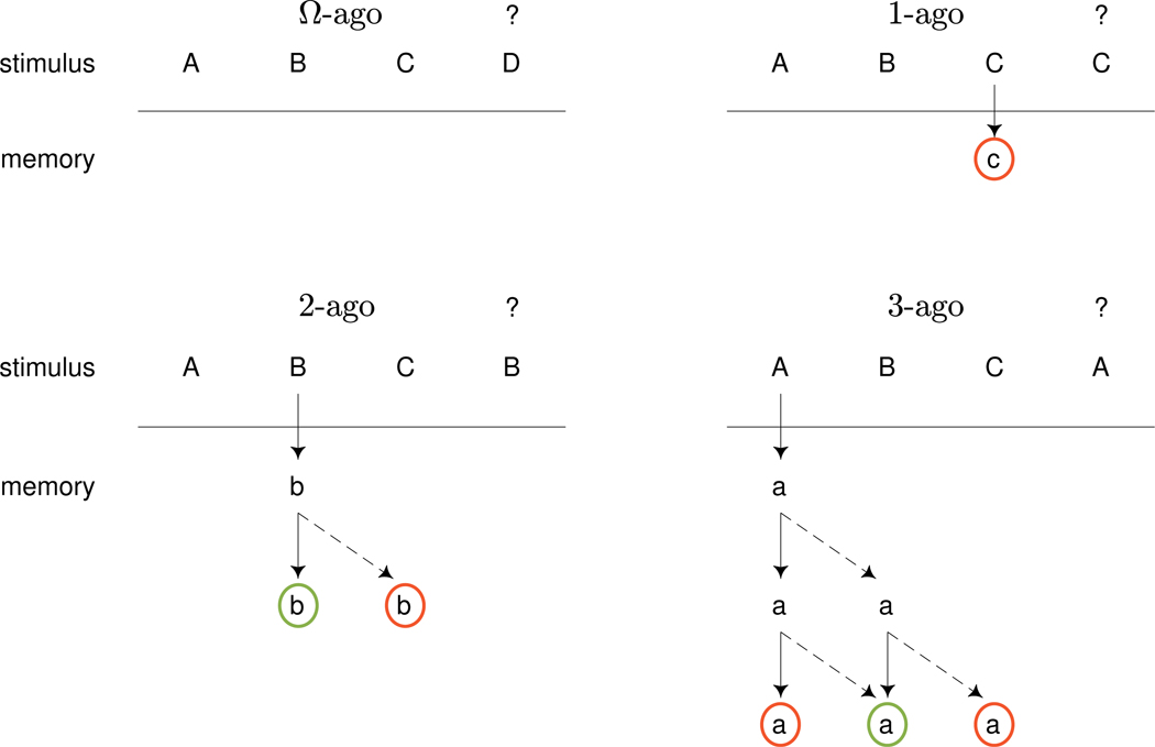
Figure 1 provides a graphical representation of the conceptual framework for our model. It shows four stimulus sequences that identify four different cases in 2-back tasks. The top-left panel shows the sequence ABCD, with the current stimulus being the final D. Since D does not appear earlier in the sequence there is no possibility it has been encoded in memory. We call this case Ω-ago (read “nullago”) because the test stimulus has not been presented recently enough for the possibility that it is in memory to be considered. In the absence of any memory signal, our modeling framework assumes a decision process operates with a base-rate of giving the correct “no” answer.

Fig. 1.

Conceptual framework for a model of 2-back task behavior. As the stimulus sequence is presented, stimuli are encoded and their positions updated. Decisions are made about the current stimulus based on the encoded stimuli and their positions

The top-right panel shows the sequence ABCC. Since the current stimulus C is presented one position earlier, there is a possibility of a memory signal. The arrow shows the possible encoding of the previous C in a slot that indicates it was presented 1-ago. The red circle indicates that this encoding sends a signal that the previous presentation was not 2-ago. Our model assumes that either the encoding does happen, in which case the “no” signal is executed with some level of accuracy, or the encoding does not happen, in which case the same base-rate decision process as for Ω-ago applies.

The bottom-left panel shows the sequence ABCB. This is the 2-ago situation for which the correct response is “yes”. The arrow shows the initial encoding of the earlier B after it was presented. At that stage in the sequence, it is encoded as 1-ago relative to the subsequent C. As the B is then presented, memory is potentially updated. The solid arrow shows this updating, with the B now correctly encoded as 2-ago. In this case, the memory signal is for a “yes” response, indicated by the green circle. It is also possible, however, that the position of the encoded B is not updated, and it continues to be considered as 1-ago. This failed updating is shown by the broken arrow. Thus, overall, there are three possibilities: the B may not be encoded at all, it may be correctly encoded as 2-ago, or it may be incorrectly encoded as 1-ago.

Finally, the bottom-right panel shows the sequence ABCA. After the original encoding of the A there are two potential updates of its position as the C and subsequent A are presented. Solid and broken arrows again indicate correct and failed updating, leading to the possibility of A being encoded as 3-, 2-, or 1-ago. Note that there are multiple routes through which the initial A can be incorrectly encoded as 2-ago at the time the current A is presented. This creates the possibility of interference, in which memory signals an incorrect “yes” response. Overall, for the 3-ago case, there are four possibilities: the A may not be encoded at all, it may be encoded correctly as a 3-ago or incorrectly as a 1-ago, both of which signal a “no” response, or it may be encoded incorrectly as a 2-ago to signal a “yes” response.

Formalization as a Multinomial Processing Tree

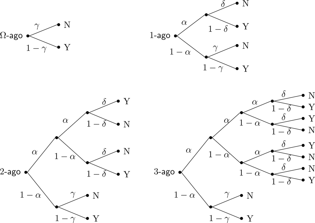
Figure 2 formalizes the 2-back task using standard probability tree notation for the $\text{Ω}$ -, 1-, 2-, and 3-ago cases. The probability of encoding a presented stimulus and successfully updating its encoded position is represented by the memory parameter $\alpha$. The probability of executing the signal provided by a remembered stimulus is represented by the accuracy-of-execution decision parameter $\delta$. The probability of responding “no” when there is no memory signal is represented by the base-rate parameter $\gamma$.

Fig. 2.

MPT model of the 2-back task, represented in terms of the $\text{Ω}$-, 1-, 2-, and 3-ago cases

The four decision trees in Fig. 2 correspond to the four cases described in Fig. 1. The trees quantify the probability of “yes” and “no” responses in each of the four cases in terms of the memory and decision parameters $\alpha ,\delta$ and $\gamma$. In the Ω-ago case, the probability of a “yes” response in the $\text{Ω}$-ago case depends only on the base-rate. We denote this probability ${\theta }_1$, and it is simply given by

$${\theta }_1=1-\gamma .$$ (1)

In the 1-ago case with the sequence ABCC, a “yes” response could be generated either by remembering the previous C with probability $\alpha$ but then inaccurately executing its signal with probability $1-\delta$, or by failing to encode the C with probability $1-\alpha$ and then producing a “yes” response following the base-rate probability $1-\gamma$. Thus, the overall probability of a “yes” response in the 1-ago case is

$${\theta }_2=\alpha (1-\delta )+(1-\alpha )(1-\gamma ).$$ (2)

The probabilities of a “yes” response for the other cases can similarly be determined by adding the products of probabilities of branches through the trees that terminate in “Y” nodes. For the 2-ago case, it is

$${\theta }_3={\alpha }^2\gamma +\alpha (1-\alpha )(1-\gamma )+(1-\alpha )(1-\gamma ),$$ (3)

and for the 3-ago case it is

$${\theta }_4={\alpha }^3(1-\gamma )+2{\alpha }^2(1-\alpha )\gamma +\alpha {(1-\alpha )}^2(1-\gamma )+(1-\alpha )(1-\gamma ).$$ (4)

Graphical Model Implementation

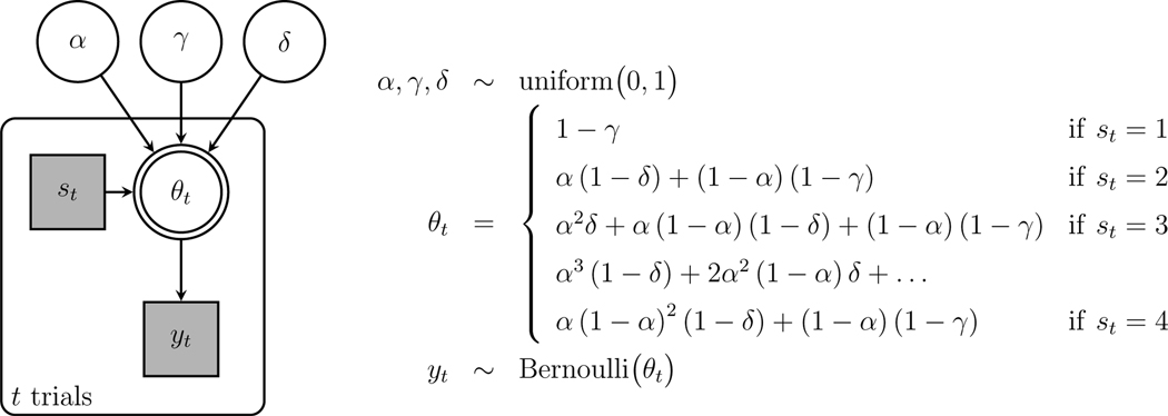
Figure 3 shows a graphical model implementation of the basic 2-back model just described. Graphical models are a language for representing probabilistic generative models developed in statistics and computer science (Jordan, 2004; Koller et al., 2007), and are increasingly widely used in cognitive science (Lee and Wagenmakers, 2013). In graphical models, nodes represent parameters and data, and the graph structure shows how they depend on each other.

Fig. 3.

Graphical model representation of the basic 2-back MPT mode

The three model parameters $\alpha ,\gamma$, and $\delta$ are shown at the top of Fig. 3. They are circular nodes, because they are continuously valued, and they are unshaded, because they are latent or unobserved. The data are shown by the $y_t$ node for the $t\text{th}$ trial, with $y_t=1$ indicating a “yes” response and $y_t=0$ indicating a “no” response. This node is square, because the values are discrete, and shaded, because the data are observed.

The model assumes the memory and decision parameters generate the observed behavioral data following the trees in Fig. 2. The probability of “yes” response on the $t\text{th}$ trial is represented by ${\theta }_t$, which takes the different values given in Equations 1–4 depending on whether the stimulus presented corresponds to a $\text{Ω}$ -, 1-, 2-, or 3-ago case. This information is represented by the discrete observed variable $s_t$, which takes the values 1, 2, 3, and 4, respectively. The dependence of the ${\theta }_t$ response probability on the parameters $\alpha ,\beta$, and $\gamma$ and the state $s_t$ is indicated by the ${\theta }_t$ node being the child of these other four parent nodes. The fact that the response probability is completely determined as a function of these other nodes is indicated by the double border around the ${\theta }_t$ node. Given this response probability, the observed response on the $t\text{th}$ trial is given by $y_t~$ Bernoulli $\left({\theta }_t\right)$ and the model is completed by uniform priors on the memory and decision parameters $\alpha ,\gamma ,\delta ~$ uniform(0,1).

We implemented all of the graphical models in this article in JAGS (Plummer, 2003), which provides a high-level scripting language, and automates the application of Markov-chain Monte Carlo methods for computational Bayesian inference. The convergence of these chains was checked via visual inspection and the standard $\widehat{R}$ statistic (Brooks and Gelman, 1997). Our results are based on 1000 or 2000 samples collected from each of 8 independent chains after up to 10,000 burn-in samples were discarded. For some applications the chains were thinned by a factor of 5.

Parameter Recovery Study

In this section, we examine some properties of the basic model in Fig. 3 using simulated data. Parameter recovery studies, in which the inferences of a model are compared to the known values that generated simulated data, are widely used in cognitive modeling. Their value as tests of models is often misunderstood (Evans & Brown 2018, p. 594; Lee 2018, pp. 42–43; Lee et al. 2019, Appendix B), but they are useful for some important purposes. Parameter recovery studies provide no information about the validity of a model and do not evaluate the assumptions of a model. They can, however, serve as checks on the correctness of implementation of a model, help diagnose potential identifiability issues with a model, and provide insight into whether behavioral data collected under specific experimental designs are likely to be informative enough to lead to useful model inferences. Our parameter recovery study addresses these three goals.

We simulated data from eight groups with ten participants each. The groups varied systematically in the $\alpha ,\gamma$, and $\delta$ values assigned to participants. Participants in four of the groups had high base-rate $\gamma$ values between 0.9 and 1, while the other four groups had low base-rates between 0.5 and 0.6. Within each of these sets of four groups, we used a 2 × 2 design with high and low values of the $\alpha$ memory and $\delta$ decision parameters. Once again, high values were between 0.9 and 1 and low values were between 0.5 and 0.6. We simulated data with each participant doing 50 experimental blocks. This corresponds to a realistic but extensive behavioral experiment.

We used three different task structures for the specific sequences of stimuli within each block. The first design used artificially created sequences of length 15. The sequences were designed so that there were significant numbers of $\text{Ω}$ -, 1-, 2-, and 3-ago cases. Specifically there were about 58% Ω-ago trials, 12% 1-ago trials, 17% 2-ago trials and 13% 3-ago trials. The second design used the length 10 stimulus sequences from the 2-back task in the Human Connectome Project (Van Essen, 2013). These sequences have about 64% Ω-ago trials, 11% 1-ago trials, 20% 2-ago trials and 5% 3-ago trials. The third design used the length 22 stimulus sequences from the 2-back task of Stelter and Degner (2018). This design is more problematic, with about 72% Ω-ago trials, 27% 2-ago trials, and fewer than 1% of both 1-ago and 3-ago trials.

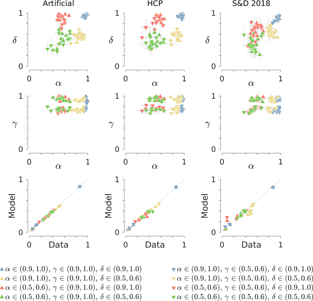
Figure 4 summarizes the results of the recovery study. The left, middle, and right columns correspond to the artificial, Human Connectome Project, and Stelter and Degner (2018) designs, respectively. The top two rows show inferred joint posterior distributions of the $\alpha$ memory parameter against the $\delta$ decision parameter and the $\gamma$ base-rate parameter. Markers indicate posterior means for each participant and error bars show interquartile credible intervals. The marker colors and shapes indicate the group membership of each participant. For the artificial and Human Connectome Project designs, it is clear that the model inferences generally match the ranges of generating parameter values for the groups. The closest match is when all three parameters have high probabilities. There is less close agreement when both $\alpha$ and $\delta$ have smaller probabilities. For the Stelter and Degner (2018) design, recovery is less effective. The difference seems likely to be caused by the very small number of 1-ago and 3-ago trials.

Fig. 4.

Summary of model inferences for simulated data with individual differences, based on artificial, Human Connectome Project (HCP) and Stelter and Degner (2018) (S&D 2018) experimental sequences

The bottom row in Fig. 4 provides a posterior predictive check of the descriptive adequacy of the model. Markers correspond to each group and each of the $\text{Ω}$ -, 1-, 2-, and 3-ago cases, showing the probability of a “yes” response given by the model’s posterior predictive distribution and the observed frequency of “yes” responses in the simulated data. There is very good agreement for all of these probabilities using the artificial and Human Connectome Project designs. Using the Stelter and Degner (2018) design leads to lower agreement, but we conclude that the model shows acceptable levels of descriptive adequacy for all three designs.

Overall, the parameter recovery study shows that the model is able to infer structured variation in the memory and decision parameters and is descriptively adequate. These results provide evidence that the model is identifiable and useful with respect to the experimental designs considered. The relatively worse performance using the Stelter and Degner (2018) design highlights the need to include all of the cases considered by the model, and more generally emphasizes the importance of experimental design in allowing model-based inferences (Cavagnaro et al., 2010; Cavagnaro et al., 2011; Myung et al., 2013).

Applications to Stelter and Degner (2018)

As a first set of applications of the model, we consider an experiment conducted by Stelter and Degner (2018). These authors used the $n$-back task as one of a set of tasks to investigate differences visual working memory between in-group and out-group face stimuli. We first show how the model can measure the memory and decision-making properties of individuals, and then show how it can test for differences with respect to the two face conditions. Specifically, we consider the data from all 52 participants in Stelter & Degner (2018, Experiment 1), which used an adaptive $n$-back procedure for blocks of 15 white and middle eastern faces. Because of this design, different participants completed different numbers of 2-back blocks, with a minimum of 1, a maximum of 10, and a mean of 3 blocks.

Measurement of Individuals

Model

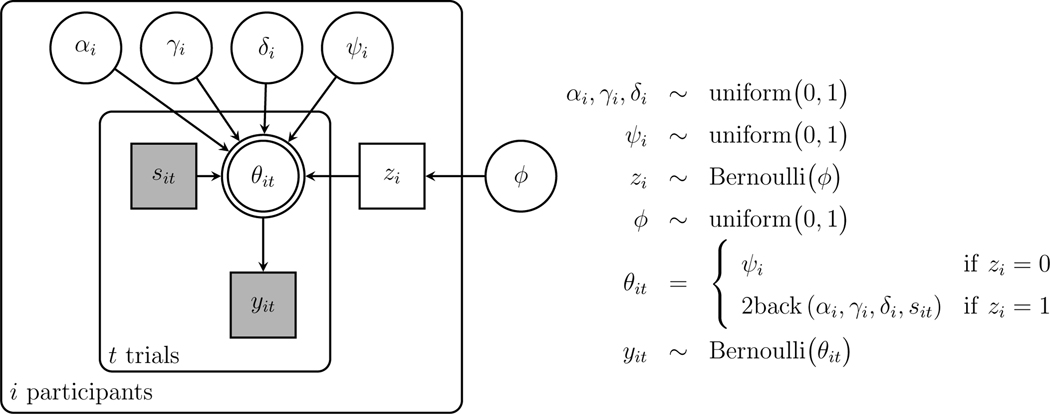
To apply the model to measure the memory and decision-making properties of individuals in an experimental setting, we extend the basic model to allow for the possibility of contaminant behavior using a latent-mixture approach (Zeigenfuse and Lee, 2010). Each participant is assumed either to make decisions according to the model on all trials, or to guess by responding “yes” with some fixed probability on all trials. If the $i\text{th}$ participant uses the model their parameters are ${\alpha }_i,{\gamma }_i$, and ${\delta }_i$, but if they guess their fixed probability is ${\psi }_i$. Which of the two possibilities is followed is determined by the indicator parameter $z_i$, with $z_i=1$ indicating model-based responses and $z_i=0$ indicating the contaminant guessing responses. The indicator parameters are sampled as $z_i~$ Bernoulli $(\varphi )$ where $\varphi$ is a population base-rate of contaminant participants with uniform prior $\varphi ~$ uniform(0,1).

The graphical model for this latent-mixture extension is shown in Fig. 5. Note that an abbreviation is used with ${\theta }_{it}=2\text{back}\left({\alpha }_i,{\gamma }_i,{\delta }_i,s_i\right)$ indicating the selection of the appropriate model response probability for ${\theta }_{it}$ depending on the case of the current trial.

Fig. 5.

Graphical model representation of the latent-mixture contaminant version of the 2-back model applied to data from Stelter and Degner (2018)

Result

All of the participants were inferred to use the model rather than the contaminant guessing process. The posterior means of the $z_i$ parameters were all greater than 0.99 and the base-rate $\varphi$ was similarly high with a mean of 0.98 and 95% credible interval (0.93,1.00). This result provides some additional evidence of the adequacy of the model in accounting for participants’ behavior. The contaminant model also provides a general approach that can be used in any analysis where it is possible some participants do not follow task instructions, or fail to perform in a motivated way.

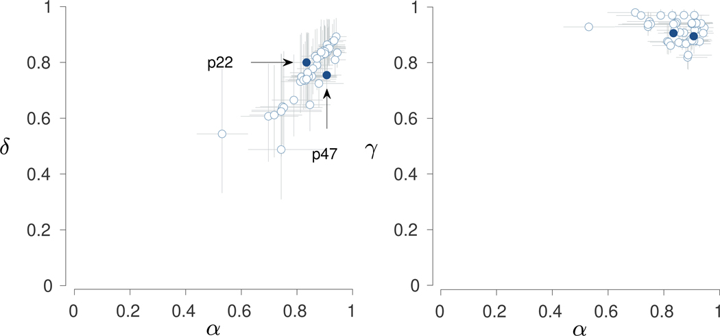
Figure 6 shows the inferred model parameters for all 52 participants. The two panels summarize the joint posterior distributions between $\alpha$ and $\delta$ and between $\alpha$ and $\gamma$. Markers correspond to posterior means and error bars show interquartile credible intervals. The posterior means show that a range of values is inferred, indicating the presence of individual differences. The credible intervals show significant uncertainty in these inferences, especially for the $\alpha$ memory and $\delta$ decision parameters. This is consistent with the relatively limited 2-back data for each individual.

Fig. 6.

Results for the 2-back conditions in Stelter and Degner (2018). The left panel shows the joint posterior between the $\alpha$ memory and $\delta$ decision parameters. The right panel shows the joint posterior between the $\alpha$ memory and $\gamma$ base-rate parameters. Points show posterior means and error bars show interquartile credible intervals. Two illustrative participants are highlighted in dark blue

Participants 22 and 47 are highlighted to demonstrate the individual differences. Participant 22 completed 10 blocks with an overall accuracy of 83%. Participant 47 completed 9 blocks and also had an overall accuracy of 83%. While their number of blocks and overall accuracies are very similar, their accuracies for the different cases are different. Participant 22 had accuracies of 91%, 100%, 61%, and 100% for Ω -, 1-, 2-, and 3-ago cases, respectively, while Participant 47 had accuracies of 90%, 50%, 69%, and 0%. The 1-ago and 3-ago cases are based on relatively few trials, because of the limitations of the experimental design. Nevertheless, these patterns suggest that Participant 22 is less accurate in identifying target 2-ago stimuli but more accurate in avoiding “yes” responses for interfering 1-ago and 3-ago matches.

The inferred $\alpha$ memory and $\delta$ decision parameters for the two participants capture this distinction. Participant 22 has ${\alpha }_{22}=0.83$ and ${\delta }_{22}=0.80$ while Participant 47 has higher ${\alpha }_{47}=0.90$ but lower ${\delta }_{47}=0.76$. Both participants have similar base-rate parameters, with ${\gamma }_{22}=0.90$ and ${\gamma }_{47}=0.89$. The model-based interpretation is that Participant 47 has better memory encoding and updating processes, which allows for better detection of target 2-ago stimuli, but worse accuracy of execution for decisions based on memory signals, which leads to errors with interfering matches in neighboring 1-ago and 3-ago positions.

Between Condition Differences

Model

To apply the model to measure differences between conditions, we distinguish between the in-group white and out-group middle eastern faces.² The goal is to test whether there are differences in the condition-level means of the parameters for responses on trials with white versus middle eastern faces.

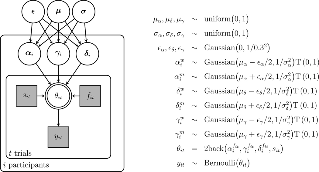
We extend the model hierarchically to allow potentially different overarching Gaussian distributions for the white and middle eastern faces. The means of these distributions are expressed in terms of a parameter representing the overall condition-level mean and a parameter representing the difference between the means for the two types of faces. For example, the overall mean for the $\alpha$ memory parameter is ${\mu }_{\alpha }$ and the difference is ${ϵ}_{\alpha }$. The condition means are then ${\mu }_{\alpha }-{ϵ}_{\alpha }/2$ for the white faces and ${\mu }_{\alpha }+{ϵ}_{\alpha }/2$ for the middle eastern faces, so that they differ by ${ϵ}_{\alpha }$.

The memory parameter used by the $i\text{th}$ participant for white faces is then sampled as

$${\alpha }_i^w~\text{Gaussian}\left({\mu }_{\alpha }-e_{\alpha }/2,\frac{1}{{\sigma }_{\alpha }^2}\right)\text{T}(0,1),$$

and for the middle eastern faces as

$${\alpha }_i^m~\text{Gaussian}\left({\mu }_{\alpha }+{ϵ}_{\alpha }/2,\frac{1}{{\sigma }_{\alpha }^2}\right)\text{T}(0,1),$$

where the standard deviation ${\sigma }_{\alpha }$ is assumed to be the same for both conditions and measures the extent of individual differences within the conditions. The T(0,1) notation denotes truncation to keep the parameters in their valid range as probabilities. The overall mean, difference, and standard deviation are given the priors ${\mu }_{\alpha }~$ uniform(0, 1), ${ϵ}_{\alpha }~$ Gaussian(0, 1∕0.3²), and ${\sigma }_{\alpha }~$ uniform(0,1). The $\delta$ decision and $\gamma$ base-rate parameters are modeled in the same way at the condition and individual level.

Figure 7 shows the graphical model representation for the face condition differences application, with each of the parameters defined with individual differences within conditions for each type of face. For the $t\text{th}$ trial, $f_{it}=1$ indicates the face is white and $f_{it}=2$ indicates the face is middle eastern. This information is used to control whether ${\alpha }_i^w,{\gamma }_i^w$, and ${\delta }_i^w$ or ${\alpha }_i^m$, ${\gamma }_i^m$, and ${\delta }_i^m$ are used to generate response probabilities according to the case of the trial. Note that the graphical model uses vectors as nodes, so that $\mathit{\mu }=\left({\mu }_{\alpha },{\mu }_{\delta },{\mu }_{\gamma }\right)$, ${\mathit{\alpha }}_i=\left({\alpha }_i^w,{\alpha }_i^m\right)$, and so on.

Fig. 7.

Graphical model representation of the between-condition differences version of the 2-back MPT model applied to data from Stelter and Degner (2018)

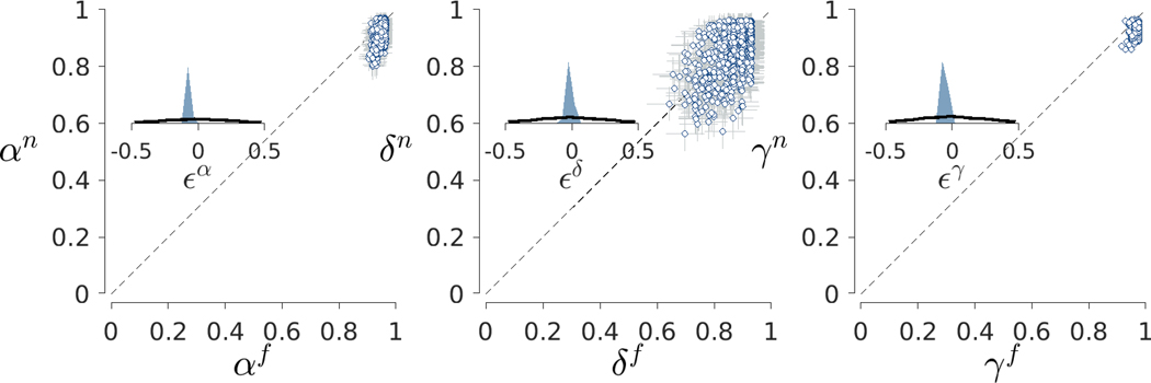
Result 2 Figure 8 shows the relationship between the inferred model parameters for white and middle eastern faces, for each of the three parameters. Each panel corresponds to a parameter, and the main scatter plot contains circular markers showing the posterior means for each participant with error bars showing interquartile credible intervals. Most participants, for all three parameters, are near the dashed diagonal line at which the parameter values for white and middle eastern faces are the same. A few participants appear possibly to have different values for ${\delta }^w$ and ${\delta }^m$ but there is no large or systematic difference across the participants as a whole.

Fig. 8.

Results for the between-condition analysis of the Stelter and Degner (2018) data. The left panel shows the relationship between the ${\alpha }^w$ and ${\alpha }^m$ memory parameters for white and middle eastern faces. Each point is a posterior mean for a participant, and error bars show interquartile credible intervals. The inset panel shows the prior (black line) and posterior (blue shaded area) distributions for the ${\in }^{\alpha }$ difference between group means. The middle and right panels show the same information for the $\delta$ decision parameters and the $\gamma$ base-rate parameters, respectively

It is interesting to note that the assumption of hierarchical individual differences, in the form of an overarching Gaussian distribution, has affected the inferences about individual parameter values through hierarchical shrinkage. This shrinkage is consistent with the uncertainty at the individual level shown in Fig. 6. Individual participant values for the $\alpha$ memory parameter, for example, span a narrower range in Fig. 8 than they do in the non-hierarchical analysis shown in Fig. 6. The hierarchical assumptions do not prevent the model from being descriptively adequate, as determined by comparing the empirically observed and posterior predicted expected probability of “yes” responses for all $\text{Ω}$ -, 1-, 2-, and 3-ago trials. The behavioral probabilities are 0.07, 0.33, 0.70, and 0.41 respectively. The model posterior predicted probabilities are 0.07, 0.20, 0.69, and 0.28. This level of agreement is very similar to that for the unconstrained model. Given the excellent agreement for the Ω-ago and 2-ago cases, which together constitute 98.7% of the trials, we regard this as an acceptable overall level of descriptive adequacy.

The inset axes in each panel in Fig. 8 show the prior and posterior distribution of the condition-level mean difference parameters. The prior is shown by the solid line and the posterior by the shaded region. For all three parameters, the posterior distributions have most of their mass close to the value zero, suggesting there is no difference between the faces in the two conditions. The Savage-Dickey method (Wetzels et al., 2010) provides a way to quantify this result by approximating the Bayes factor between the null model of no difference in the condition means and the alternative model of a difference. The Bayes factor is approximated as the ratio of posterior to prior density at the critical value $ϵ=0$. For all three parameters, the Bayes factor favors the null, with values of about 3, 2, and 14 for $\alpha ,\delta$, and $\gamma$ respectively. We interpret these results as providing weak evidence of no difference for the $\alpha$ memory and $\delta$ decision parameters, and strong evidence of no difference for the $\gamma$ base-rate parameter. The finding of no evidence for differences due to the type of face, and some evidence for sameness, is consistent with the results in Stelter & Degner (2018, Figure 1), which showed that the accuracy for the two types of faces is very similar for the 2-back blocks.

Applications to the Human Connectome Project

As a second set of applications of the model, we consider behavioral data from the Human Connectome Project young adult data set (Van Essen, 2013).³ The Human Connectome Project data set contains behavioral and neuroimaging data from 1200 young adults on a variety of cognitive tasks and assessments, with the broad purpose of understanding human brain structure, function, and connectivity and their relationships to behavior. One of the Human Connectome Project tasks is the 2-back working memory task.

We consider three applications of our model to these data. The first is a measurement application, with the same goals as for the Stelter and Degner (2018) data. The second is an application to between-condition differences. In the Human Connectome Project 2-back task, participants complete eight blocks with 10 trials each, and there are four types of stimuli: faces, tools, bodies, and places. One stimulus type is used for each block. Previous studies have suggested a visual short-term memory advantage for faces compared to non-face objects (Curby and Gauthier, 2007). In the context of the 2-back task, no consensus has emerged regarding concrete performance differences in faces versus non-face objects, although distinct cortical regions have been implicated in the processing of face, body parts, places, and tools as stimuli (Barch, 2013). Not hampered by small sample sizes, the Human Connectome Project data is ideal to evaluate a model-based account of whether there are process- and performance-related differences in face versus non-face stimuli. Thus, we test whether there are differences in model parameters between the face and non-face stimuli. Finally, we develop a new application that regresses model parameters on cognitive measures derived from other tasks in the Human Connectome Project behavioral battery. There are 1082 participants in the data set with valid 2-back task data and complete external task measures. All three analyses are conducted on these participants.

Measurement of Individuals

Model

We again use the graphical model shown in Fig. 5, including the contaminant guessing process.

Result

All of the 1082 participants were again inferred to use the model rather than the contaminant guessing process. The posterior means of the $z_i$ parameters were all greater than 0.98 and the base-rate $\varphi$ has posterior density concentrated near 1 with a mean of 0.999 and 95% credible interval of (0.996,1.000).

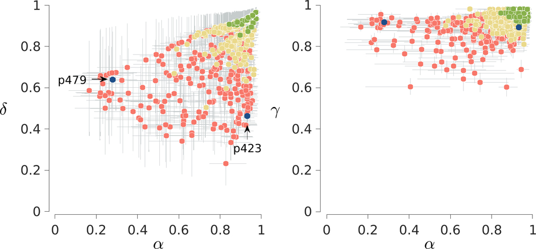
Figure 9 shows the inferred model parameters for all participants. As before, the two panels summarize the joint posterior distributions between $\alpha$ and $\delta$ and between $\alpha$ and $\gamma$. Markers correspond to posterior means and error bars show interquartile credible intervals. Markers are now colored to indicate three categories of accuracy, with the most accurate 25% of participants with better than 92% correct in green, the least accurate 25% of participants with worse than 80% accuracy in red, and the remaining moderate accuracy 50% of participants in yellow.

Fig. 9.

Results for the 2-back task in the Human Connectome Project. The left panel shows the joint posterior between the $\alpha$ memory and $\delta$ decision parameters. The right panel shows the joint posterior between the $\alpha$ memory and $\gamma$ base-rate parameters. Markers show posterior means and are colored to indicate the 25% lowest accuracy (red), 50% moderate accuracy (yellow) and 25% highest accuracy (green) participants. Error bars show interquartile credible intervals. Two illustrative participants are also highlighted

It is clear that highly accurate participants have, unsurprisingly, both good memory and decision execution, with all three model parameters close to 1. As accuracy decreases, a range of individual differences emerges and, once again, there is significant uncertainty about the values of the $\alpha$ and $\delta$ parameters. Participants 479 and 423 are highlighted to demonstrate these individual differences. Both completed the standard 8 blocks and they had accuracies of 69% and 72% respectively. Their accuracies for the different cases are, however, very different. Participant 479 had accuracies of 82%, 78%, 19%, and 75% for $\text{Ω}$ -, 1-, 2-, and 3-ago cases, respectively. This means that they missed many target 2-ago stimuli, but were reasonably accurate in saying “no” to non-target stimuli. Participant 423, in contrast, had accuracies of 86%, 11%, 81%, and 0%. This participant is better at identifying targets, but makes more errors also saying “yes” to interfering 1-ago and 3-ago stimuli.

The inferred $\alpha$ memory and $\delta$ decision parameters for the two participants capture this distinction. Participant 479 has ${\alpha }_{479}=0.28$ and ${\delta }_{479}=0.64$ while Participant 423 has higher ${\alpha }_{423}=0.93$ but lower ${\delta }_{423}=0.46$. Both participants have similar base-rate parameters, with ${\gamma }_{479}=0.92$ and ${\gamma }_{423}=0.89$. As with the previous analysis of illustrative participants in Fig. 6, the model-based interpretation is that Participant 479 has better memory encoding and updating processes, which allows for better detection of target 2-ago stimuli, but worse accuracy of execution of decisions based on memory signals. This inferior decision-making leads to errors with interfering matches in neighboring 1-ago and 3-ago positions.

Between Condition Differences

Model

We again use the graphical model shown in Fig. 7. The only adjustment that is needed is to define the two conditions. For the $t\text{th}$ trial, $f_{it}=1$ indicates a face stimulus and $f_{it}=2$ indicates one of the other stimulus types.

Result 4 As before, we checked the descriptive adequacy of the hierarchical model. The behavioral probabilities are 0.06, 0.10, 0.81, and 0.40, respectively, for $\text{Ω}$ -, 1-, 2-, and 3-ago trials. The model posterior predicted probabilities are 0.06, 0.12, 0.77, and 0.20. Given the relatively small number (fewer than 5%) of 3-ago trials, we regard this as an acceptable overall level of descriptive adequacy.

Figure 10 shows the relationship between the inferred model parameters for the face (${\alpha }^f,{\delta }^f$, and ${\gamma }^f$) and non-face (${\alpha }^n,{\delta }^n$, and ${\gamma }^n$) stimuli. The main scatter plots use circular markers to show the posterior means for each participant with error bars showing interquartile credible intervals. Once again, all three parameters, but especially the $\alpha$ and $\delta$ parameters, show evidence of hierarchical shrinkage compared to the independent individual-level inferences.

Fig. 10.

Results for the between-condition analysis of the Human Connectome Project data. The left panel shows the relationship between the ${\alpha }^f$ and ${\alpha }^n$ memory parameters for face and non-face stimuli. Each point is a posterior mean for a participant, and error bars show interquartile credible intervals. The inset panel shows the prior (black line) and posterior (blue shaded area) distributions for the ${\in }^{\alpha }$ difference between group means. The middle and right panels show the same information for the $\delta$ decision parameters and the $\gamma$ base-rate parameters, respectively

In terms of differences between stimulus types, participants seem to vary roughly symmetrically around the dashed diagonal line of equality for the decision $\delta$ parameter. For the memory $\alpha$ parameter, however, it seems clear that values are systematically greater for faces compared to non-face stimuli. The same pattern appears to be true for the base-rate $\gamma$ parameter, although all values are much closer to one. Bayes factors support this interpretation of the visual patterns. A Bayes factor of 10 favors the null hypothesis of no difference between for $\delta$, but Bayes factors both greater than 1000 favor the alternative hypothesis of a difference for the $\alpha$ and $\gamma$ parameters.

This suggests a novel psychometric result in the 2-back task, with a distinct advantage emerging in the $\alpha$ memory parameter but not the $\delta$ decision parameter for face versus non-face stimuli. Such a distinct difference for face-related memories has not been measured within the 2-back working memory task, although previous studies have suggested a visual short-term memory advantage for faces compared to non-face objects in other working memory tasks (Curby and Gauthier, 2007).

Regression on External Measures

To demonstrate how the model can analyze the relationship between model parameters and external tasks measures, we consider four external cognitive assessment tasks. The first is the Penn Matrix reasoning task (Moore et al., 2015; Bilker et al., 2012), which is intended to measure abstraction and non-verbal reasoning in complex cognition using a set of matrix reasoning problems similar to the Raven’s (1989) progressive matrices. The remaining three tasks—the List Sort working memory task, the Card Sort dimensional change task, and the Flanker inhibitory control and attention task—are part of cognition assessment using the NIH toolbox (Weintraub, 2013). The List Sort task is intended to test working memory and involves sequencing pictures of animals and foods, presented together with a text name and a sound, in order of their size. The Card Sort task is intended to measure executive function and cognitive flexibility. It involves matching test pictures and target pictures with two dimensions. The pictures have two dimensions, such as shape and color, and matching must first be done according to one dimension and then to the other. The Flanker task (Eriksen and Eriksen, 1974) is intended to measure attention and inhibitory control and requires attending to a target stimulus and inhibiting attention to surrounding stimuli that may be incongruent. The stimuli are fish or arrows, and congruency or incongruency is determined by the direction in which the target and flanking stimuli point.

The motivation for this application is to evaluate the selective association between these cognitive assessments and the cognitive parameters inferred by our model of 2-back task behavior. Importantly, we do this using a joint modeling approach where the relationships are inferred within a hierarchical Bayesian framework simultaneously with inference about the model parameters, rather than a two-stage correlational approach (Turner et al., 2019). This has the advantage of incorporating uncertainty in the parameter estimates while inferring the relationships (Matzke et al., 2017).

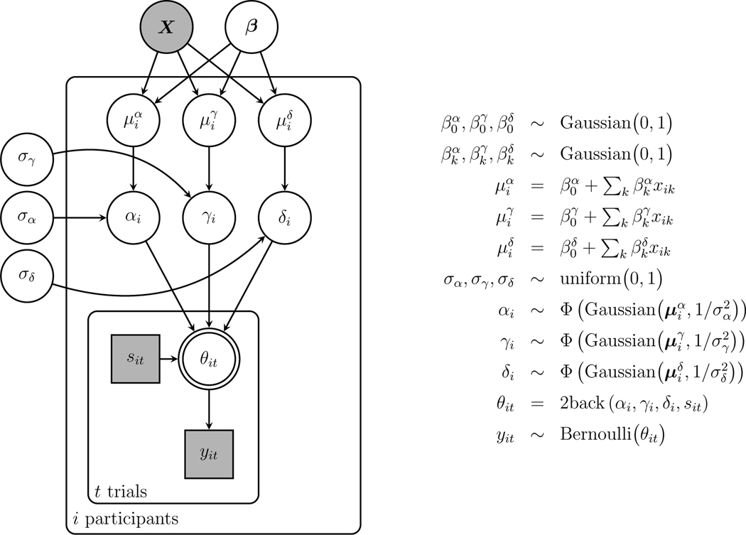
Model To examine the relationship between parameters and external measures, we use a multivariate regression approach. The basic idea is that each of the ${\alpha }_i,{\delta }_i$, and ${\gamma }_i$ parameters for the $i\text{th}$ participant are modeled as being systematically related, via the linear combination specified by the regression model, to their performance on the other external tasks. Formally, this is achieved by assuming the individual-level parameters are noisy samples from a Gaussian distribution centered on a weighted linear combination of the external measures. For example, the memory parameter ${\alpha }_i$ is sampled as

$${\alpha }_i~\text{Φ}\left(\text{Gaussian}\left({\mu }_i^{\alpha },1/{\sigma }_{\alpha }^2\right)\right).$$

The probit transformation $\text{Φ}(\cdot )$ converts the sample from the Gaussian distribution into a probability on the interval from 0 to 1. The standard deviation ${\sigma }_{\alpha }$ corresponds to the level of noise, and is assumed to be the same for all participants, The ${\mu }_i^{\alpha }$ is the participant-specific mean given by the linear combination

$${\mu }_i^{\alpha }={\beta }_0^{\alpha }+\sum _k{\beta }_k^{\alpha }{x}_{ik}.$$

In this equation, $x_{ik}$ is the measure for the $i\text{th}$ participant on the $k\text{th}$ external task, ${\beta }_k^{\alpha }$ is the weight given to the $k\text{th}$ task, and ${\beta }_0^{\alpha }$ is a constant. The external measures are normalized as z-scores. The regression weights are given standard priors ${\beta }_0^a,{\beta }_k^a~$ Gaussian(0,1) and the noise is given the uniform prior ${\sigma }_{\alpha }~$ uniform(0,1). As shown in the graphical model in Fig. 11, the ${\delta }_i$ and ${\gamma }_i$ are defined similarly, with their own regression weights and level of noise.

Fig. 11.

Graphical model representation of the multivariate regression version of the 2-back MPT model applied to data from the Human Connectome Project

Result

It is especially important to examine the descriptive adequacy of the regression model, to ensure that the linear combination constraints still allow for individual-level parameters consistent with observed behavior according to the basic 2-back model. We again compare the empirically observed and posterior predicted expected probability of “yes” responses for all $\text{Ω}$ -, 1-, 2-, and 3-ago trials. There is excellent agreement for the first three cases, but not as good agreement for the 3-ago trials. As before, the behavioral probabilities are 0.06, 0.10, 0.81, and 0.40 respectively. The model posterior predicted probabilities are 0.06, 0.10, 0.76, and 0.20, which we continue to regard as adequate.

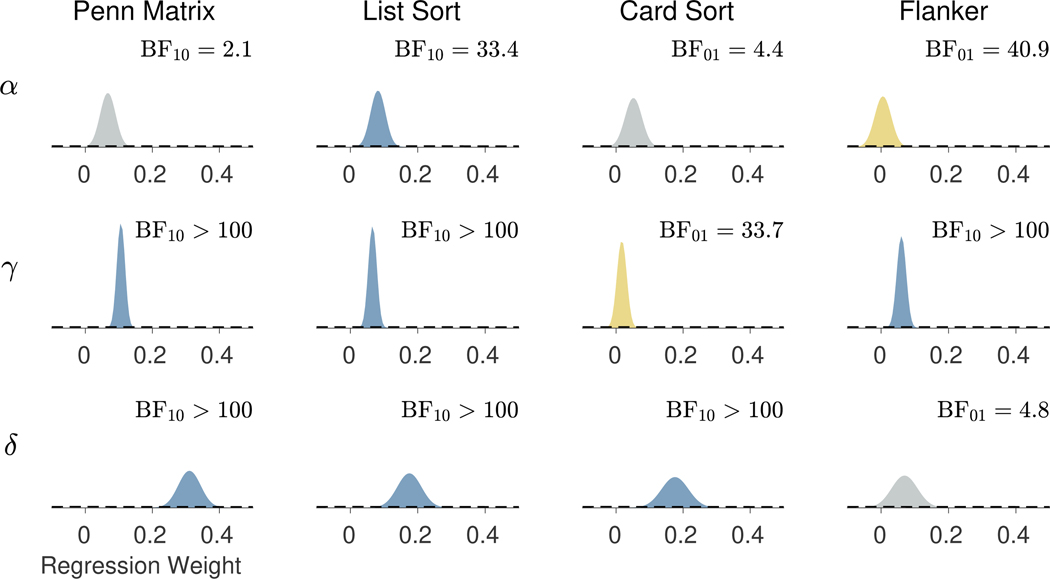
Figure 12 shows the inferred regression weights relating each model parameter, in rows, to each external task, in columns. The posterior and prior distributions are shown, and the Bayes factor comparing the null hypothesis of no difference to the alternative hypothesis of a difference is listed. These Bayes factors are expressed in terms of the hypothesis they favor, so that BF₀₁ corresponds to evidence in favor of the null, and BF₁₀ corresponds to evidence in favor of the alternative. The posterior distributions are colored according to the Bayes factor, with blue posteriors indicating strong evidence for a relationship ( BF₁₀ >10 ), yellow posteriors indicating strong evidence for no relationship ( BF₀₁ >10 ), and gray posteriors indicated no strong evidence for either hypothesis.

Fig. 12.

Prior and posterior distributions for the regression weights for each model parameter, in rows, and external task, in columns. The prior distributions are shown by broken lines and posterior distribution is shown by the shaded areas. The Bayes factor comparing the null hypothesis of no difference to the alternative hypothesis of a difference is listed. The posterior distributions are colored according to the Bayes factor in terms of strong evidence for a relationship (blue), strong evidence for no relationship (yellow), or no strong evidence either way (gray)

There is strong evidence the List Sort task is related to the $\alpha$ memory parameter, with BF₁₀ = 33.4. The posterior mean of the regression weight is 0.08 with a 95% credible interval (0.04,0.12). All of the external tasks except the Card Sort task are significantly related to the $\gamma$ base-rate parameter, all with BF₁₀ >100. The posterior means and credible intervals are 0.11 (0.08,0.13) for the Penn Matrix task, 0.07 (0.04,0.09) for the List Sort task, and 0.06 (0.03,0.09) for the Flanker task. All of the external tasks except the Flanker task are significantly related to the $\gamma$ base-rate parameter, with BF₁₀ >100 in each case. These relationships have relatively larger regression weights. The posterior means and credible intervals are 0.31 (0.25,0.38) for the Penn Matrix task, 0.18 (0.11,0.24) for the List Sort task, and 0.18 (0.10,0.25) for the Card Sort task.

The regression results suggest a number of interpretable relationships. First, only the List Sort task measure, which assesses working memory, shows a significant relationship with the memory parameter $\alpha$. This is consistent with the notion that $\alpha$ captures the core memory component of the 2-back process. Further, the List Sort task measure has significant relationships with both the decision-making and base-rate parameters, $\delta$ and $\gamma$, which reflects the fact that both the 2-back and List Sort tasks measure working memory and can be expected to require similar underlying cognitive capabilities. Secondly, the Penn Matrix task is a measure of fluid intelligence, and this is reflected in a strong association with both the decision-making and base-rate parameters, $\delta$ and $\gamma$, but inconclusive evidence with respect to the memory parameter $\alpha$. Thirdly, the Card Sort task, which measures cognitive flexibility, shows a significant positive relationship only with the $\delta$ decision parameter. The decision parameter represents the ability to discriminate a valid internal memory signal. There is some limited evidence of such an association between cognitive flexibility and the ability to detect signals, although these were external rather than internal signals (Figueroa and Youmans, 2012). Finally, the Flanker task, which measures sensitivity to attention and inhibitory control, shows a significant relationship only with the $\gamma$ base-rate parameter. A possible interpretation of the base-rate parameter is as the rate of inhibiting a pre-potent “yes” response when no memory signal is detected, thus sharing inhibitory capabilities with that demonstrated in the Flanker task.

Discussion

The main goal of our model is as a psychometric instrument to measure the memory and decision-making components of 2-back task behavior. We aimed to achieve this via a generative cognitive modeling approach, by making assumptions about how latent cognitive parameters lead to observable task behavior.

Broader Interpretation of Model Parameters

The $n$-back task is popular largely because it combines memory processes of encoding, retrieval, and updating with decision processes related to inhibition and control in one simple task. Thus, it is natural to ask how the parameters in our model relate to existing psychological constructs related to these cognitive capabilities. In general, answers to these questions require applying the model to relevant experimental data that measures the other constructs and $n$-back behavior in a within-participants design. Given this experimental evidence, our regression application provides a template for how the relationship between our model parameters and external task measures can be investigated in a statistically principled way. It would be possible to extend this joint modeling approach further by incorporating process models of the other task being related to $n$-back behavior (Turner et al., 2019). Future work should explore how tasks relating to working memory, cognitive control, temporal binding, and other relevant cognitive capabilities are related to the measures of $n$-back behavior our model provides using the full power of joint modeling approaches.

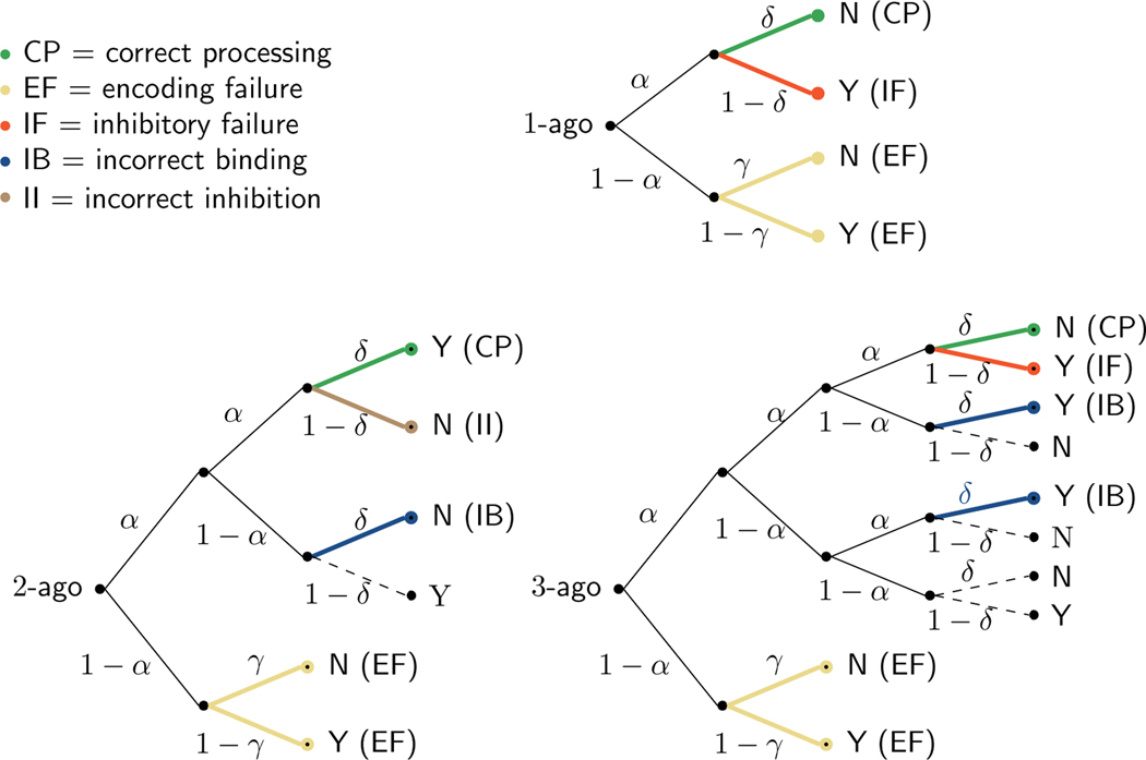
As an initial speculative framework to guide investigating these theoretical relationships, Fig. 13 presents one interpretation of the different branches of our MPT model. This interpretation classifies different processing possibilities as corresponding to correct processing, an encoding failure, an inhibitory failure, an incorrect inhibition, or an incorrect binding. Final branches in the 1-ago, 2-ago, and 3-ago trees are colored and labeled according to the appropriate category, or presented as dashed edges if the interpretation is unclear.

Fig. 13.

Interpretation of the MPT model in terms of five broad theoretical concepts: correct processing, encoding failures, inhibitory failures, incorrect bindings, and incorrect inhibitions. The 1-ago, 2-ago, and 3-ago trees are shown, with the final branch colored to indicate which of these concepts applies. Paths that are difficult to interpret are shown as dashed edges

For each classification type, we calculated the expected proportion of trials based on parameter posterior means for both the Stelter and Degner (2018) data and the Human Connectome Project data. Correct processing occurs when memory encoding, updating, and retrieval all function as required by the task and a correct response is produced. This is the most common expected outcome, accounting for 67%, 58%, and 51% for the 1-ago, 2-ago, and 3-ago trials in the Stelter and Degner (2018) data, and 74%, 66%, and 59% of trials in the Human Connectome Project data. Encoding failures occur when a stimulus is not stored in memory at the time it is presented. The model infers that this occurs on about 14% of trials in both data sets. Inhibitory failure occurs when the item is encoded and its position correctly updated, but an incorrect decision is made at the final stage. The model infers this accounts for about 19% and 13% of 1-ago and 3-ago trials for the Stelter and Degner (2018) data, and correspondingly 13% and 9% of trials for the Human Connectome Project data. Incorrect binding occurs when an item is encoded but there is a failure at some point in the updating process, resulting in an incorrect binding between the stimulus and the context provided by its position in the sequence (Ranganath, 2010). The model infers that incorrect binding accounts for 9% and 15% of 2-ago and 3-ago trials for the Stelter and Degner (2018) data, and correspondingly 8% and 13% for the Human Connectome Project data. Incorrect binding does not affect the 1-ago trials since no contextual updating is involved. Finally, incorrect inhibition can occur only in the 2-ago case, where the correct “yes” answer is inhibited. The model infers that this occurs on 16% of the 2-ago trials in the Stelter and Degner (2018) data and 11% in the Human Connectome Project data. Full details on this analysis for all of the paths through all of the trees are available in the supplementary material.

The analysis in Fig. 13 emphasizes how the MPT approach dissects observed behavior into interpretable components. According to the model and the inferred parameters, correct responses are most likely to result from accurate encoding, updating, and responding, and much less likely to result from guessing the correct answer after an encoding failure. As detailed above, correct responses are inferred to result from correct processing on about 50 to 60% of trials. Correct guessing after failed encoding is inferred to occur on only slightly over 12% of trials when the correct answer is “no” and only about 1% of trials when the correct answer is “yes”. In terms of incorrect “yes” responses in the 3-ago case, the model explains just under half as being caused by binding failures, just under half as being caused by inhibition failures, and only a few as being caused by encoding failures. This differs from the 2-ago case, where encoding failures account for almost a third of the errors made. This sort of breakdown highlights the usefulness of the model in dissociating the processes that contribute to individual differences in interference effects as well as correct responding.

It is interesting to note that, cumulatively, the interpretable possibilities account for the majority of trials. The final branches in the 2-ago and 3-ago trees that are difficult to interpret, at least in terms of existing working memory and cognitive control theory, have much lower probability, collectively accounting for no more than about 5% of trials. This is an encouraging result in terms of the psychological interpretability of the model. It suggests that the classification of paths into the classes of correct processing, encoding failure, inhibitory failure, incorrect binding, and incorrect inhibition provides a useful theoretical framework for understanding the cognitive variables and processes involved in $n$-back tasks, and their potential relationship to related variables and processes in other tasks.

Additional theoretical resolution could potentially be achieved by extending our model to account for response times as well as choice behavior. Response times for $n$-back tasks are routinely analyzed statistically, and potentially provide additional insight into the cognitive processes underlying behavior. A framework for this extension is provided by Klauer and Kellen (2018), who develop a general approach for extending MPT models to include response times. The basic idea is to associate response time distributions with each edge of the probability tree, and define the total observed response time as being the sum of component response times along the branch that produced the behavior. The potential theoretical resolution offered by an extension to response times is made clear by considering the relationship between the parameters in our model and the model measures and the sub-processes described by Rac-Lubashevsky and Kessler (2016) in their $n$-back analysis. Their “updating cost” sub-process roughly corresponds to the role of the $\alpha$ memory parameter in maintaining the relative positions of encoded stimuli on each trial, and their “matching” sub-process roughly corresponds to the role of the $\delta$ decision parameter comparing the presented stimulus to one stored in memory. Similarly, their “intrusion” measure is captured by the interference effects constituting a subset of the MPT branches. The different sub-processes are assumed to contribute separately to response times, consistent with the Klauer and Kellen (2018) framework. The “substitution”, “gate opening”, and “gate closing” sub-processes in Rac-Lubashevsky and Kessler (2016), however, go beyond the parameters in our model, because they correspond to parameters obtained from a modified reference-back task that allows measurement of additional processes. The substitution mechanism corresponds roughly to the part of $\alpha$ that measures the probability of initial encoding. The gate-opening and gate-closing mechanisms seem to capture the switching between trials that need updating rather than maintenance in a modified reference task. A potential extension of our model would involve identifying separate tree structures for switch versus non-switch trials, and then identifying appropriate branches that correspond to the gate-opening and gate-closing mechanism in each. All of these finer-grained distinctions would benefit from extending the model to make predictions about response time distributions, or applying it to more complex $n$-back tasks (e.g., 6-back tasks), or both.

The final important challenge is to explore the neural correlates of the dissociated process parameters, beyond the neural correlates typically measured for accuracy and reaction time (Li et al., 2021). This may provide greater functional resolution in understanding how different brain regions and connectivity link to the separate memory and decision-making processes.

Limitations and Extensions

Our MPT framework account of $n$-back models is general and could be used to formulate specific models other than for 2-back tasks. We do not believe, however, that the 1-back model based on the framework is well identified. In a model recovery evaluation, similar to the one reported here for the 2-back model, the 1-back model failed to recover meaningful variation in generating parameters. We believe this limitation arises because of the lack of sufficient cases to distinguish the different decision parameters. We believe that the 2-back model is effective, in part, because of the presence of both 1-ago and 3-ago cases surrounding the target 2-back case. The relatively poor recovery performance of the 2-back model using the Stelter and Degner (2018) experimental design, which has very limited 1-ago and 3-ago cases, is consistent with this conclusion. Accordingly, our expectation is that the conceptual framework should lead to effective models for 3-back tasks and beyond, but we have not implemented and tested these models.

An assumption of the conceptual framework is that an earlier stimulus that matches the currently presented one is unique among those being considered as potentially in memory. For example, in the 3-ago case considered in Fig. 1, the first A potentially interferes with the current A, but the stimuli between these presentations are different from A. This is a reasonable assumption for most $n$-back experiments, which use a large number of stimuli and present each relatively infrequently. Some $n$-back experiments, however, use as few as two stimuli, and thus repeat them often (e.g., Rac-Lubashevsky and Kessler, 2016). This violates the basic assumption of just considering the most recent stimulus that matches the current one, if such a stimulus exists, in formulating the $\text{Ω}$ -, 1-, 2-, and 3-ago cases. It is not clear how well our framework and model will apply to these experimental designs.

In both of our applications of hierarchical extensions of the model we observed significant shrinkage. This is likely due to the relatively limited information about the model parameters provided by the experimental designs. To the extent these designs are typical, however, the extent of shrinkage observed should lead to some caution. Individual differences need to be carefully incorporated in the model, and the resulting inferences compared with those found by applying the model independently to individuals. For many applications, it may be better to apply the model independently rather than hierarchically, using the sort of approach adopted for the regression application.

Finally, there is scope for exploring variants of the basic model. The current assumption is that both the initial encoding of a presented stimulus and its later latent position updating occur with the same probability. We tested that this was a good assumption for the data we modeled but, as mentioned earlier, it seems theoretically plausible that these probabilities may sometimes be different. It also seems reasonable to consider a more complicated model in which the updating probabilities change from trial to trial, as the time increases since the relevant stimulus was presented. This may be especially important for more difficult $n$-back tasks with larger $n$ and higher cognitive load. These tasks are more likely to produce data that will allow dissociable measurements of initial encoding and subsequent updating.

Conclusion

We developed and demonstrated a simple psychometric model of the widely used 2-back working memory tasks, using the MPT modeling framework. Consistent with the MPT modeling philosophy and dissecting cognitive processes into simple branching steps controlled by probabilities, our model treats 2-back behavior as arising from a memory and encoding probability that remembers stimuli and their relative position to the current stimulus, and decision and base-rate probabilities that lead to “yes” or “no” responses depending on the signals (or lack of signals) provided by memory. The model does not aim to be a detailed account of 2-back behavior, but aims instead to provide a simple and useful characterization of individual performance. As our applications show, the basic model can serve as the core of more elaborate models that are tailored to specific data and research questions, including measurement, comparison across task and stimulus conditions, and regression analyses of the relation between latent 2-back working memory measures and standardized cognitive measures of working memory, reasoning and response inhibition.

Availability of Data and Materials

The data sets and additional analysis are available in an Open Science Framework repository at https://osf.io/esxhf/.

References

- Au J, Sheehan E, Tsai N, Duncan GJ, Buschkuehl M, & Jaeggi SM (2015). Improving fluid intelligence with training on working memory: a meta-analysis. Psychonomic Bulletin & Review, 22, 366–377. [DOI] [PubMed] [Google Scholar]
- Barch DM, et al. (2013). Function in the human connectome: task-fMRI and individual differences in behavior. Neuroimage, 80, 169–189. [DOI] [PMC free article] [PubMed] [Google Scholar]
- Batchelder WH, & Riefer DM (1999). Theoretical and empirical review of multinomial process tree modeling. Psychonomic Bulletin & Review, 6, 57–86. [DOI] [PubMed] [Google Scholar]
- Bilker WB, Hansen JA, Brensinger CM, Richard J, Gur RE, & Gur RC (2012). Development of abbreviated nine-item forms of the Raven’s standard progressive matrices test. Assessment, 19, 354–369. [DOI] [PMC free article] [PubMed] [Google Scholar]
- Brooks SP, & Gelman A. (1997). General methods for monitoring convergence of iterative simulations. Journal of Computational and Graphical Statistics, 7, 434–455. [Google Scholar]
- Cai W, Ryali S, Pasumarthy R, Talasila V, & Menon V. (2021). Dynamic causal brain circuits during working memory and their functional controllability. Nature Communications, 12, 1–16. [DOI] [PMC free article] [PubMed] [Google Scholar]
- Cavagnaro DR, Myung JI, Pitt MA, & Kujala JV (2010). Adaptive design optimization: A mutual information-based approach to model discrimination in cognitive science. Neural Computation, 22, 887–905. [DOI] [PubMed] [Google Scholar]
- Cavagnaro DR, Pitt MA, & Myung JI (2011). Model discrimination through adaptive experimentation. Psychonomic Bulletin & Review, 18, 204–210. [DOI] [PMC free article] [PubMed] [Google Scholar]
- Chatham CH, Herd SA, Brant AM, Hazy TE, Miyake A, O’Reilly R, & Friedman NP (2011). From an executive network to executive control: A computational model of the n-back task. Journal of Cognitive Neuroscience, 23, 3598–3619. [DOI] [PMC free article] [PubMed] [Google Scholar]
- Coulacoglou C. & Saklofske DH (2017). Psychometrics and psychological assessment: Principles and applications. Academic Press. [Google Scholar]
- Curby KM, & Gauthier I. (2007). A visual short-term memory advantage for faces. Psychonomic Bulletin & Review, 14, 620–628. [DOI] [PubMed] [Google Scholar]
- Ecker UK, Lewandowsky S, Oberauer K, & Chee AE (2010). The components of working memory updating: an experimental decomposition and individual differences. Journal of Experimental Psychology: Learning, Memory, and Cognition, 36, 170–189. [DOI] [PubMed] [Google Scholar]
- Erdfelder E, Auer T-S, Hilbig BE, Aßfalg A, Moshagen M, & Nadarevic L. (2009). Multinomial processing tree models: A review of the literature. Zeitschrift für Psychologie/Journal of Psychology, 217, 108–124. [Google Scholar]
- Eriksen BA, & Eriksen CW (1974). Effects of noise letters upon the identification of a target letter in a nonsearch task. Perception & Psychophysics, 16, 143–149. [Google Scholar]
- Evans NJ, & Brown SD (2018). Bayes factors for the linear ballistic accumulator model of decision-making. Behavior research methods, 50, 589–603. [DOI] [PubMed] [Google Scholar]
- Figueroa IJ & Youmans RJ (2012). Individual differences in cognitive flexibility predict performance in vigilance tasks. In Proceedings of the human factors and ergonomics society annual meeting, volume 56 (pp. 1099–1103).: SAGE Publications Sage CA: Los Angeles, CA. [Google Scholar]
- Guastello SJ, Reiter K, Malon M, Timm P, Shircel A, & Shaline J. (2015). Catastrophe models for cognitive workload and fatigue in N-back tasks. Nonlinear Dynamics, Psychology, and Life Sciences, 19, 173–200. [PubMed] [Google Scholar]
- Harbison J, Atkins SM, & Dougherty MR (2011). N-back training task performance: Analysis and model. In Carlson L, Hölscher C, & Shipley TF (Eds.), Proceedings of the 33rd Annual Conference of the Cognitive Science Society (pp. 120–125). Austin, TX: Cognitive Science Society. [Google Scholar]
- Harvey P-O, et al. (2005). Cognitive control and brain resources in major depression: An fMRI study using the n-back task. Neuroimage, 26, 860–869. [DOI] [PubMed] [Google Scholar]
- Jaeggi SM, Buschkuehl M, Jonides J, & Perrig WJ (2008). Improving fluid intelligence with training on working memory. Proceedings of the National Academy of Sciences, 105, 6829–6833. [DOI] [PMC free article] [PubMed] [Google Scholar]
- Jordan MI (2004). Graphical models. Statistical Science, 19, 140–155. [Google Scholar]
- Juvina I. & Taatgen NA (2007). Modeling control strategies in the n-back task. In Proceedings of the 8th International Conference on Cognitive Modeling (pp. 73–78).: Psychology Press; New York. NY. [Google Scholar]
- Kirchner WK (1958). Age differences in short-term retention of rapidly changing information. Journal of Experimental Psychology, 55, 352. [DOI] [PubMed] [Google Scholar]
- Klauer KC, & Kellen D. (2018). RT-MPTs: Process models for response-time distributions based on multinomial processing trees with applications to recognition memory. Journal of Mathematical Psychology, 82, 111–130. [Google Scholar]
- Koller D, Friedman N, Getoor L, & Taskar B. (2007). Graphical models in a nutshell. In Getoor L. & Taskar B. (Eds.), Introduction to Statistical Relational Learning. Cambridge, MA: MIT Press. [Google Scholar]
- Lee MD (2018). Bayesian methods in cognitive modeling. In Wixted J. & Wagenmakers E-J (Eds.), The Stevens’ Handbook of Experimental Psychology and Cognitive Neuroscience. Volume 5: Methodology chapter 2, (pp. 37–84). John Wiley & Sons, fourth edition. [Google Scholar]
- Lee MD, Gluck KA, & Walsh MM (2019). Understanding the complexity of simple decisions: Modeling multiple behaviors and switching strategies. Decision, 6, 335–368. [Google Scholar]
- Lee MD & Wagenmakers E-J (2013). Bayesian cognitive modeling: A practical course. Cambridge University Press. [Google Scholar]
- Li G, Chen Y, Le TM, Wang W, Tang X, & Li C-SR (2021). Neural correlates of individual variation in two-back working memory and the relationship with fluid intelligence. Scientific reports, 11, 1–13. [DOI] [PMC free article] [PubMed] [Google Scholar]
- Mackworth JF (1959). Paced memorizing in a continuous task. Journal of Experimental Psychology, 58, 206. [DOI] [PubMed] [Google Scholar]
- Matzke D, Ly A, Selker R, Weeda WD, Scheibehenne B, Lee MD, & Wagenmakers E-J (2017). Bayesian inference for correlations in the presence of measurement error and estimation uncertainty. Collabra: Psychology, 3, 25. [Google Scholar]
- Moore TM, Reise SP, Gur RE, Hakonarson H, & Gur RC (2015). Psychometric properties of the Penn Computerized Neurocognitive Battery. Neuropsychology, 29, 235. [DOI] [PMC free article] [PubMed] [Google Scholar]
- Myung JI, Cavagnaro DR, & Pitt MA (2013). A tutorial on adaptive design optimization. Journal of Mathematical Psychology, 57, 53–67. [DOI] [PMC free article] [PubMed] [Google Scholar]
- Owen AM, McMillan KM, Laird AR, & Bullmore E. (2005). N-back working memory paradigm: A meta-analysis of normative functional neuroimaging studies. Human Brain Mapping, 25, 46–59. [DOI] [PMC free article] [PubMed] [Google Scholar]
- Patterson F, et al. (2009). Varenicline improves mood and cognition during smoking abstinence. Biological Psychiatry, 65, 144–149. [DOI] [PMC free article] [PubMed] [Google Scholar]
- Plummer M. (2003). JAGS: A program for analysis of Bayesian graphical models using Gibbs sampling. In Hornik K, Leisch F, & Zeileis A. (Eds.), Proceedings of the 3rd International Workshop on Distributed Statistical Computing (DSC 2003). [Google Scholar]
- Rac-Lubashevsky R, & Kessler Y. (2016). Decomposing the n-back task: An individual differences study using the reference-back paradigm. Neuropsychologia, 90, 190–199. [DOI] [PubMed] [Google Scholar]
- Ranganath C. (2010). Binding items and contexts: The cognitive neuroscience of episodic memory. Current Directions in Psychological Science, 19, 131–137. [Google Scholar]
- Raven J. (1989). The Raven Progressive Matrices: A review of national norming studies and ethnic and socioeconomic variation within the United States. Journal of Educational Measurement, 26, 1–16. [Google Scholar]
- Schmiedek F, Li S-C, & Lindenberger U. (2009). Interference and facilitation in spatial working memory: Age-associated differences in lure effects in the n-back paradigm. Psychology and Aging, 24, 203. [DOI] [PubMed] [Google Scholar]
- Schoofs D, Preuß D, & Wolf OT (2008). Psychosocial stress induces working memory impairments in an n-back paradigm. Psychoneuroendocrinology, 33, 643–653. [DOI] [PubMed] [Google Scholar]
- Stelter M, & Degner J. (2018). Investigating the other-race effect in working memory. British Journal of Psychology, 109, 777–798. [DOI] [PubMed] [Google Scholar]
- Sylvester J, Reggia J, Weems S, & Bunting M. (2013). Controlling working memory with learned instructions. Neural Networks, 41, 23–38. [DOI] [PubMed] [Google Scholar]
- Turner BM, Forstmann BU, spsampsps Steyvers M. (2019). A tutorial on joint modeling. Joint Models of Neural and Behavioral Data, (pp. 13–37). [Google Scholar]
- Van Essen DC, et al. (2013). The WU-Minn human connectome project: an overview. Neuroimage, 80, 62–79. [DOI] [PMC free article] [PubMed] [Google Scholar]
- Weintraub S, et al. (2013). Cognition assessment using the NIH Toolbox. Neurology, 80, S54–S64. [DOI] [PMC free article] [PubMed] [Google Scholar]
- Wetzels R, Grasman RPPP, & Wagenmakers E. (2010). An encompassing prior generalization of the Savage-Dickey density ratio test. Computational Statistics and Data Analysis, 54, 2094–2102. [Google Scholar]
- Zeigenfuse MD, & Lee MD (2010). A general latent assignment approach for modeling psychological contaminants. Journal of Mathematical Psychology, 54, 352–362. [Google Scholar]
Associated Data
This section collects any data citations, data availability statements, or supplementary materials included in this article.
Data Availability Statement