Integration of single cell RNA-sequencing and network analysis to investigate mechanism of drug resistance

Abstract

Innate resistance and therapeutic-driven development of resistance to anti-cancer drugs is a common complication of cancer therapy. Understanding mechanisms of drug resistance can lead to development of alternative therapies. One strategy is to subject drug sensitive and resistant variants to single-cell RNA-seq (scRNA-seq) and subjecting the scRNA-seq data to network analysis to identify pathways associated with drug resistance. This protocol describes a computational analysis pipeline to study drug resistance by subjecting scRNA-seq expression data to Passing Attributes between Networks for Data Assimilation (PANDA), an integrative network analysis tool that incorporates protein-protein interactions (PPI) and transcription factor (TF)-binding motifs.

1). Introduction

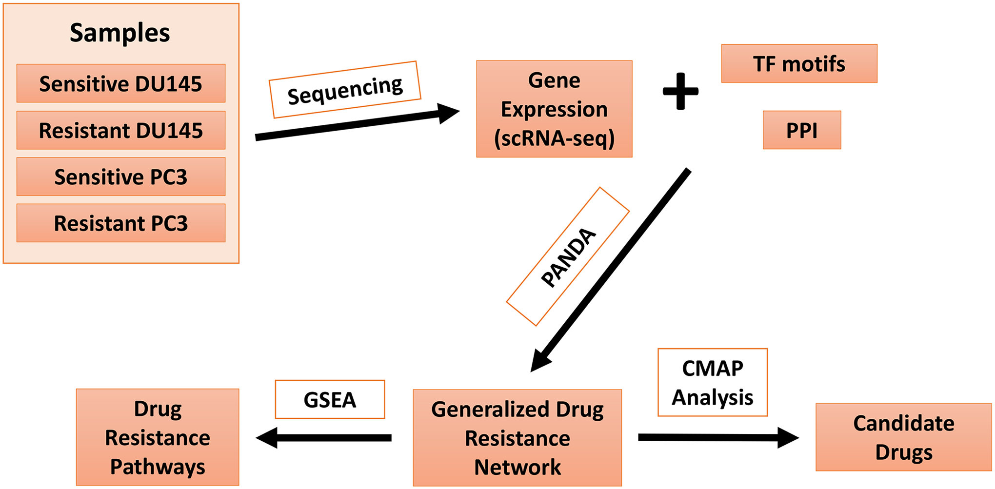
Drug resistance is a frequent therapeutic challenge when attempting to treat cancer patients. Many cancer studies have attempted to identify other drugs and therapies to overcome drug resistance and increase the chance of survival in various cancer patients (1). The majority of these studies tend to focus on a few genes and examine their change in expression due to drug resistance (1). Furthermoe, they tend to only look at one data type or multiple data types separately. This limits the ability to fully understand the mechanisms underlying drug resistance. To increase the possibility to determine how drug resistance develops and subsequently identify alternative therapies, gene regulatory network modeling, which can integrate multiple data types, should be considered. Passing Attributes between Networks for Data Assimilation (PANDA) is an integrative network analysis tool, which uses a message-passing model to iterate over multiple data types to predict regulatory relationships (2,3). Specifically, PANDA integrates gene expression, protein-protein interactions (PPI), gene co-regulation, and transcription factor (TF)-binding motif data. Single-cell RNA-seq (scRNA-seq) is a powerful technique that allows us to study the transcriptome of variable and heterogenous cell populations on a single-cell level, which cannot be examined with traditional bulk sequencing (1). Incorporating scRNA-seq data into PANDA may lead to an enhanced understanding of mechanisms of drug resistance and identify new, alternative therapies to overcome this resistance. The described protocol will provide a general analysis pipeline to identify regulatory networks, pathways association with these regulatory networks, and discover alternative drugs that could potentially overcome drug resistance. This general pipeline (Figure 1) was composed and used with previous studies (1,4).

Figure 1.

General Network Analysis Pipeline. Sensitive and resistant samples are subjected to scRNA-seq, followed by subjecting the scRNA-seq data in combination with transcription factor (TF) motifs and protein-protein interactions (PPI), derived from established databases, to PANDA analysis. This will lead to identifications of a generalized drug resistance network which can then be subjected to gene set enrichment analysis (GSEA) and connectivity map analysis (CMAP) to identify drug resistance pathways and candidate drugs, respectively.

2). Materials

2.1). Software (see Note 1)

1. R

   1. R is an open-source programming coding language mainly used for statistical analysis and graphics (5).
   2. Information on and download R here: https://www.r-project.org/
   3. Additional packages needed:

      1. Seurat (https://satijalab.org/seurat/)

         1. Seurat is an R package used to analyze quality control (QC) and exploration of scRNA-seq data (6).
      2. wordcloud2 (https://github.com/lchiffon/wordcloud2)

         1. wordcloud2 is an R package used to create word clouds for data visualizations (7).
2. Passing Attributes between Networks for Data Assimilation (PANDA) (2)

   1. Download the bash version here: http://sourceforge.net/projects/panda-net/files/Version2/Version2.tgz/download
   2. Read the “README.txt” to compile the C++ scripts and run the commands PANDA and AnaPANDA. Also, read this file to find more information on how the input files need to be structured.
3. Find Individual Motif Occurrences (FIMO)

   1. FIMO is a program used to search and extract sequences that match independent motifs provided (8).
   2. Download the MEME suite, which contains FIMO, here: https://meme-suite.org/meme/doc/download.html
   3. Install the MEME suite. You can find installation instructions here: https://meme-suite.org/meme/doc/install.html?man_type=web
   4. To run FIMO, you can find the manual here: https://meme-suite.org/meme/doc/fimo.html
4. Gene Set Enrichment Analysis (GSEA)

   1. GSEA is a computation method that is commonly used for pathway analysis. It determines if a set of genes that are different between two biological states is statistically significant for a set of pathways (9,10).
   2. Download and install GSEA here: https://www.gsea-msigdb.org/gsea/doc/GSEAUserGuideTEXT.htm#_Starting_GSEA
   3. The link above also contains the manual to run GSEA both on command line and GUI program.

2.2). Datasets

1. Gene expression dataset

   1. General structure:

      1. Gene expression, done with scRNA-seq, from at least two cell lines are required. Each cell line requires at least two conditions (ex: sensitive vs. resistant). In total, there should be at least four samples (two cell lines, each with a sensitive and resistant variant).
      2. The counts in the gene expression dataset from every sample should be normalized.
      3. Since the dataset will have multiple single cells per sample, the normalized counts should be combined into “pseudo-bulk” counts for each gene for each sample for the dataset to work in PANDA. Some methods to combine the normalized single cell counts per condition are by averaging, summation, scoring, etc. These “pseudo-bulk” counts will then be used in PANDA.
      4. This new matrix must be structured as genes (as rows) by samples (as columns) and exported as tab delimited .txt file.
   2. Example:

      1. Raw counts can be found here: https://www.ncbi.nlm.nih.gov/geo/query/acc.cgi?acc=GSE140440
      2. The example expression gene dataset used for this protocol is based on another previous study we published (11). Briefly, this dataset contains gene expression of single cells from two prostate cancer (PCa) cell lines, Du145 (DU145) and PC-3 (PC3). There was a parental (docetaxel-sensitive) and docetaxel-resistant variant for each cell line. In the end, there was four conditions: sensitive DU145, resistant DU145, sensitive PC3, and resistant PC3. For more information about the experiment and sequencing, please refer to this study’s paper (11) (see Note 2).
      3. The single cell counts from all conditions were normalized together using the log normalization method (NormalizeData) in Seurat. The normalized counts were then aggregated into “pseudo-bulk” counts per condition. In this example, the matrix had genes as rows and conditions as columns, which there was four columns.
2. TF motif prior dataset

   1. General structure:

      1. A TF motif dataset needs to be downloaded that matches the species of the gene expression dataset (see Note 3). For example, if the gene expression dataset is from Mus musculus, then you will need a TF motif dataset specific to Mus musculus. This dataset will contain all the motifs found in this species.
      2. The full TF motif dataset needs to be filtered for TFs found in the gene expression dataset. FIMO can be used to get these motifs.

         1. A sequence file is needed (in fasta format) for the dataset’s species to run FIMO.
         2. To run FIMO, refer to the link in the Software section in 3d.
   2. Example:

      1. The Homo Sapiens TF motifs dataset was downloaded from the. This dataset contains all the TF motifs found in Homo Sapiens (see Note 4).
      2. A sequence file (in .fasta format) was also downloaded. For this study, the human genome assembly dataset GRCh37 (also called hg19) was used (https://genome.ucsc.edu/cgi-bin/hgTables).
      3. The TF motifs position weight matrices were mapped to using FIMO.
      4. A TF motif prior specific to the expression dataset was created by only using the TFs found in the expression dataset. There was 240 TFs in this example TF motif prior dataset.
3. PPI files

   1. General structure:

      1. A PPI dataset needs to be downloaded that contains interaction scores.
      2. The interaction scores need to be between 0 and 1. The scores will need to be transform if they are not already in this format. Any self-interactions need to be set equal to one.
   2. Example:

      1. The example PPI dataset that contains interaction scores was downloaded from StringDb v10.5 (see Note 4). This dataset contains interactions from all data sources in StringDb.
      2. The interaction scores were then divided by 1000 for the scores to be between 0 and 1. The self-interactions were set equal to one.

3). Methods

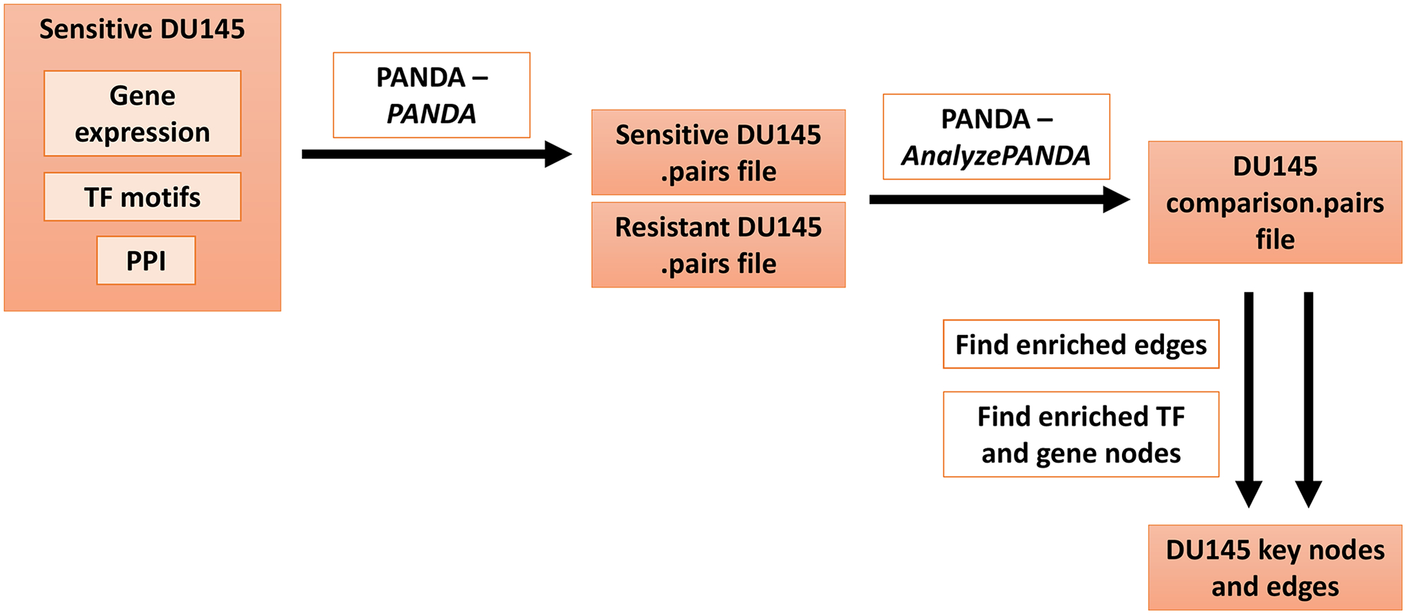
Steps 3.1 through 3.6 are delineated in Figure 2.

Figure 2.

Overview of steps for generating a key network for one cell line. This figure describes steps 3.1–3.6 of the protocol. Details are found within the protocol text. TF=transcription factor, PPI=protein-protein interactions.

• 3.1)
  Constructing PANDA regulatory networks

  1. Create a TF regulatory network for each condition using the TF motif prior, PPI, and the expression dataset from Material section. A code example is:

     ./Version2/PANDA -e express_data/DU145_sen.txt -m motif_data/TF_motif.txt -p PPI_data/PPI.txt -o networks/DU145_sen
     

     From this command, you should have four FinalNetwork.pairs files.
• 3.2)
  Compare PANDA networks

  1. Within each cell line, compare networks in the FinalNetwork.pairs files from step 3.1 with PANDA with the example code below:

     ./Version2/AnalyzePANDA_v0/AnalyzePANDA -a DU145_resist_FinalNetwork.pairs -b DU145_sen_FinalNetwork.pairs -P 0.8 -o DU_resist_vs_sen
     

     From this command, there should be two sets of five comparison network files. In this example, there was one comparing resistant and sensitive cells from the DU145 cell line, and another comparing resistant and sensitive cells from the PC3 cell line. Each set should have a FinalNetwork.pairs, RankedList_for_GSEA.rnk, Gene_degree_comparison.txt, TF_degree_comparison.txt, and Subnetworks.pairs files.
• 3.3)
  Finding enriched edges

  1. Over all the networks (all), calculate the median (med) and IQR for each edge weight (w) between each TF (t) and gene (g) from the FinalNetwork.pairs files from step 3.1.
  2. For each edge weight in each network (n), calculate a specificity score (s). In general, we compare the weight to the median and IQR for each TF-gene found in the last step. The equation to calculate scores is shown below (4):

     $$s_{tg}^{\left(c\right)}=\left(w_{tg}^{\left(c\right)}-med\left(w_{tg}^{\left(all\right)}\right)\right)/IQR\left(w_{tg}^{\left(all\right)}\right)$$
  3. Determine enriched edges. An edge is enriched for a network if s > N where N is a threshold for a specificity score over all networks. N was found through calculating the specificity score for each individual gene and comparing those scores to the median and IQR across all networks. The specificity score can vary between 0 and 1. For this study, we found that N = 0.4 where half of the genes were enriched.
• 3.4)
  Finding enriched TF nodes

  1. For each network, calculate the in-degree of each TF node, which is the sum of enriched edges connected to a TF node. The enriched edges are from the TF_degree_comparison.txt files from step 3.2.
  2. Calculate p-values to test differences of in-degree values for each TF node between conditions in either cell line using a hypergeometric distribution. In this example, p-values were calculated between sensitive and resistant cells in either DU145 or PC3 cell lines
  3. Calculate the edge weight fold change using the in-degree value for each node between the two networks.
  4. Determine enriched TF nodes. In this example, these were determined as enriched for a cell line if they had a p-value than 0.05 (p < 0.05).
• 3.5)
  Finding enriched gene nodes

  1. The process is the same as finding enriched TF nodes in step 3.4, except using the Gene_degree_comparison.txt files from step 3.2.
• 3.6)
  Finding key TF and gene node

  1. We followed the following criteria to find key TF and gene nodes:

     1. The node must have a p-value (found in step 3.4 or 3.5) less than 0.05 (p < 0.05) for both cell line network comparisons. In this example, a specific node must both have p < 0.05 in both DU145 and PC3 cell lines.
     2. The node must have an edge weight fold change (found in step 3.4 or 3.5) in the same direction for both cell line network comparisons, for instance, the fold change must be positive in both comparisons. In this example, a specific node must have an edge weight fold change in the same direction in both DU145 and PC3 cell lines.

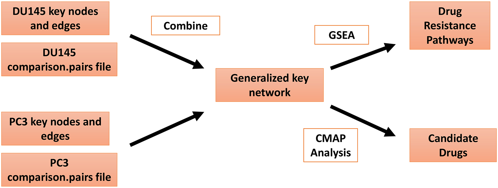
Steps 3.7 through 3.9 are delineated in Figure 3.

Figure 3.

Overview of process for generating a generalized key network and further downstream analysis. This figure describes steps 3.7–3.9 of the protocol. Details are found within the protocol text. GSEA=gene set enrichment analysis, CMAP=connectivity map.

• 3.7)
  Creating a generalized network

  1. Combine common key edges and nodes that were identified from step 3.6 to create a generalized network. For this study, this network represents prostate cancer response to docetaxel treatment between DU145 and PC3 cell lines.
• 3.8)
  GSEA of TF specific-targeted genes

  1. Create a pre-ranked gene list using the specificity scores of each TF that was calculated in step 3.4.
  2. Run pre-ranked GSEA on GO terms with the pre-ranked gene list. Pathways that were considered as enriched if they had a false discovery rate (FDR) less than 0.05 (FDR < 0.05).
  3. Cluster the significant pathways using hierarchical clustering.
  4. For each cluster, calculate the frequency of each word that appeared in the GO terms.
  5. Calculate p-values to test word enrichment using a hypergeometric probability. P-values were scaled by using -log10, which the most statistically relevant words would be the largest.
  6. Create word clouds for each cluster with the words from the pathway names. The size of the words is determined by the -log10(p) values.
• 3.9)
  Connectivity map (CMAP) analysis

  1. Go to the CMAP website here: https://portals.broadinstitute.org/cmap. (see Note 5 before going to website) (12).
  2. Label the gene nodes as a certain condition based on their edge weight fold change found in step 3.6. In this example, the gene nodes were labeled as either sensitive or resistant.
  3. Run the gene nodes list from the last step in CMAP to predict response in various drugs. These drugs should either up-regulate sensitive gene nodes and down-regulate resistant gene nodes. In this example, drugs with positive enrichment would mean that these drugs had the highest potential to reverse docetaxel resistance in PCa.

4). Notes

1. The tools used in this protocol can be run on multiple different platforms and coding languages. Alternative versions or coding languages are acceptable to use. Please use the most up-to-date software for all tools mentioned.

2. The scRNA-seq method to create the example expression dataset is very old. However, the analysis pipeline explained in this protocol can be used with current scRNA-seq methods.

3. You can find motif datasets in Catalog of Inferred Sequencing Bind Preferences (CIS-BP), MEME (https://meme-suite.org/meme/db/motifs), etc.

4. The PPI and TF motif datasets used as examples are older versions of what can be found today. Please use the most up-to-date datasets.

5. The CMAP website used for this analysis is not available anymore. The CMAP dataset has moved here: https://clue.io/. For information about the algorithm, please refer to [12].

References

- 1.Schnepp PM et al. (2021) Transcription factor network analysis based on single cell RNA-seq identifies that Trichostatin-a reverses docetaxel resistance in prostate Cancer. BMC Cancer 21. doi: 10.1186/s12885-021-09048-0 [DOI] [PMC free article] [PubMed] [Google Scholar]
- 2.Glass K et al. (2013) Passing messages between biological networks to refine predicted interactions. PLoS One 8(5). doi: 10.1371/journal.pone.0064832 [DOI] [PMC free article] [PubMed] [Google Scholar]
- 3.Glass K et al. (2015) A network model for angiogenesis in ovarian cancer. BMC Bioinformatics 16. doi: 10.1186/s12859-015-0551-y [DOI] [PMC free article] [PubMed] [Google Scholar]
- 4.Sonawane AR (2017) Understanding Tissue-Specific Gene Regulation. Cell Rep 21(4):1077–1088. doi: 10.1016/j.celrep.2017.10.001 [DOI] [PMC free article] [PubMed] [Google Scholar]
- 5.R Core Team (2022) R: A language and environment for statistical computing. R Foundation for Statistical Computing. https://www.R-project.org/ [Google Scholar]
- 6.Hao Y et al. (2021) Integrated analysis of multimodal single-cell data. Cell 184(13): 3573–3587. doi: 10.1016/j.cell.2021.04.048 [DOI] [PMC free article] [PubMed] [Google Scholar]
- 7.Dawei L, Guan-tin C (2018) wordcloud2: Create Word Cloud by ‘htmlwidget’. R package version 0.2.1. https://CRAN.R-project.org/package=wordcloud2
- 8.Grant CE et al. (2011) FIMO: Scanning for occurrences of a given motif. Bioinformatics 27(7):1017–1018. doi: 10.1093/bioinformatics/btr064 [DOI] [PMC free article] [PubMed] [Google Scholar]
- 9.Subramanian A et al. (2005) Gene set enrichment analysis: a knowledge-based approach for interpreting genome-wide expression profiles. PNAS 102:15545–15550. doi: 10.1073/pnas.0506580102 [DOI] [PMC free article] [PubMed] [Google Scholar]
- 10.Mootha V et al. (2003) PGC-1α-responsive genes involved in oxidative phosphorylation are coordinately downregulated in human diabetes. Nat Genet 34:267–273. doi: 10.1038/ng1180 [DOI] [PubMed] [Google Scholar]
- 11.Schnepp PM et al. (2020) Single-cell transcriptomics analysis identifies nuclear protein 1 as a regulator of docetaxel resistance in prostate Cancer cells. Mol Cancer Res 18:1290–1301. doi: 10.1158/1541-7786.MCR-20-0051 [DOI] [PMC free article] [PubMed] [Google Scholar]
- 12.Lamb J et al. (2006) The connectivity map: using gene-expression signatures to connect small molecules, genes, and disease. Science 313:1929–1935. doi: 10.1126/science.1132939 [DOI] [PubMed] [Google Scholar]