Abstract
The enormous social and economic cost of Alzheimer’s disease (AD) has driven a number of neuroimaging investigations for early detection and diagnosis. Towards this end, various computational approaches have been applied to longitudinal imaging data in subjects with Mild Cognitive Impairment (MCI), as serial brain imaging could increase sensitivity for detecting changes from baseline, and potentially serve as a diagnostic biomarker for AD. However, current state-of-the-art brain imaging diagnostic methods have limited utility in clinical practice due to the lack of robust predictive power. To address this limitation, we propose a flexible spatial-temporal solution to predict the risk of MCI conversion to AD prior to the onset of clinical symptoms by sequentially recognizing abnormal structural changes from longitudinal magnetic resonance (MR) image sequences. Firstly, our model is trained to sequentially recognize different length partial MR image sequences from different stages of AD. Secondly, our method is leveraged by the inexorably progressive nature of AD. To that end, a Temporally Structured Support Vector Machine (TS-SVM) model is proposed to constrain the partial MR image sequence’s detection score to increase monotonically with AD progression. Furthermore, in order to select the best morphological features for enabling classifiers, we propose a joint feature selection and classification framework. We demonstrate that our early diagnosis method using only two follow-up MR scans is able to predict conversion to AD 12 months ahead of an AD clinical diagnosis with 81.75% accuracy.
Keywords: Early AD diagnosis, Longitudinal MRI, Machine Learning, Temporal Structured Support Vector Machine
I. INTRODUCTION
Alzheimer’s disease (AD) is often primed by isolated memory dysfunction referred to as Mild Cognitive Impairment (MCI), followed by progressive decline in general cognitive abilities, altered behavior, loss of functional independence, and eventually death (Grimmer et al., 2009; Lam et al., 2013; Loewenstein et al., 2006). Although AD cannot be stopped or cured, the most effective way to treat AD patients is to slow AD progression in the early stage (Chetelat & Baron, 2003; Filley, 1995; Gauthier, 2005). Therefore, detecting the early onset of AD symptom is critically important for the success of AD treatments in clinical practice. The structural and functional loss involved in AD are known to have dynamically evolving morphological patterns (Duchesne et al., 2008; C. R. Jack et al., 2003; Klöppel et al., 2008; Vemuri et al., 2009; Whitwell et al., 2008). These dynamic brain structural changes can be captured by noninvasive longitudinal MR imaging data. Therefore, early AD diagnosis using longitudinal imaging has been documented in previous work with special attention to MCI (Cummings et al., 2007; M. Ganguli et al., 2010; Mary Ganguli et al., 2004; Johnson et al., 2009; Li et al., 2012; Petersen, 2000; Reisberg et al., 2008; Winblad et al., 2004). MCI entails noticeable and measurable cognitive changes that are not severe enough to interfere with daily life or independent function, and carries an increased risk of developing AD or other type of dementia.
A growing body of research has set focus on attempting to predict if and when MCI patients will convert to AD. For example, tensor-based morphometry (Hua et al., 2011; Hua et al., 2010) is used to identify brain atrophy patterns in 91 AD patients and 189 MCI subjects scanned at baseline, 6, 12, 18, and 24 months. Since the hippocampus is a primary locus of early AD pathologic changes, many studies have investigated structural changes involving the hippocampal region. For example, Lee and colleagues employed a linear regression model to predict MCI conversion using hippocampus surface morphology and several clinical indices (Lee et al., 2015). Examining longitudinal changes in hippocampal volume (Chincarini et al., 2016) and cortical thickness (Li et al., 2012) are other approaches that have been used in an attempt to identify predictor variables of MCI conversion to AD.
A major general limitation of computer-assisted longitudinal AD diagnostic methods is the scanning protocol used with respect to the timing and number of scans obtained. For example, many longitudinal approaches assume the number of time points is equal, albeit implicitly. In clinical practice, however, patients will have a variable number of scans, often fewer than are obtained in longitudinal studies, and typically not done more frequently than annually. Moreover, each subject recruited in the Li and colleagues study (Li et al., 2012) should have at least 5 time-points at 6-month intervals, and should develop AD at least 12 months after the baseline scan. Hence, existing methods typically require a large number of MRI scans in order to be robust. Regarding the time window prior to the onset of AD clinical symptoms, conventional methods can only support predictive modeling over a relatively short time frame, even when a number of longitudinal scans are available. For instance, the imaging classification method used by Li and colleagues (Li et al., 2012) accurately predicted MCI to AD conversion only 6 months before the clinical expression of AD symptoms. Although the short-term prediction result seems promising, signaling conversion to AD only 6 months before the clinical syndrome appears would have limited impact on clinical practice based on convergent evidence that early and continuous treatment confers a therapeutic advantage relative to patients for whom treatment initiation is delayed for disrupted (Gauthier, 2005).
Several works utilizing computer vision have shown promise in early activity detection (Hoai et al., 2011; Hoai & Torre, 2014; Huang et al., 2014). Early activity detection in these works involves first training detectors to specifically recognize any small partial activities from the complete activities. The detection score of those partial activities are then constrained to increase monotonically along with time since those partial activities are conducted continuously. Inspired by the success of early activity detection in computer vision, we propose a long-range AD early detection approach that requires only a few MR scans.
The goal of our approach is to detect AD associated brain changes before the clinical diagnosis of AD. Accordingly, we regard the problem of AD early diagnosis as a binary classification task between MCI converters (MCI-C for short) who convert from MCI to AD and MCI non-converters (MCI-NC for short) who do not progress to AD. We leverage the following facts to achieve long range early diagnosis with only a few longitudinal MR scans: (1) AD progression is irreversible (Filley, 1995), and (2) the disparity of morphological patterns between MCI-C and MCI-NC become more manifest with AD progression (Hua et al., 2011; Thompson et al., 2007). In light of this, we will provide a principled mechanism to achieve this monotonicity in AD early diagnosis, which is not obtained by any existing diagnostic approaches. The assumption of monotonicity on AD conversion score is based on AD progression model in [43], which shows that the AD progression begins at a stimulating time point where the brain structure start to changes from normal to abnormal monotonically follows a sigmoid shape curve. Moreover, the study in [43] also reveal that the brain structure changes measured by structural MRI is an earlier biomarker than clinical scores test. This finding suggests that longitudinal MRI data are better early AD diagnosis biomarker than clinical score based AD diagnosis. Therefore, we present to study the longitudinal MRI imaging data using a Temporally Structured SVM (TS-SVM) to capture the brain structural changes during AD progression. Our model is trained based on a set of partial MR image sequences at variable intervals, drawn from the complete longitudinal imaging data. Note, partial image sequencing not only augments the set of training samples but also harnesses the inclusion relationship within partial sequences to reflect the inexorably progressive nature of AD by requiring the risk of AD conversion to monotonically increase as AD progresses. Compared with conventional SVM, our TS-SVM has three major improvements to achieve long-range early AD detection with high accuracy:
The classifier is trained to recognize all partial MR image sequences and is therefore not restricted by the number of available MR images or AD progression stage.
We require the AD conversion score to monotonically increase within each AD-converting MCI subject as more follow-up images are inspected. Thus, our early diagnosis method can avoid inconsistent prediction results
We balance the early prediction accuracy and prediction range of AD conversion. Since the monotonicity makes the risk of future AD conversion more predictable, we have greater confidence to signal the future conversion of AD much earlier than the onset of clinical symptoms. Another benefit is that we can reduce number of MR scans, which is very important for translation to routine clinic practice.
We further present a joint feature selection and classification framework in order to select suitable features that are in line with the learned TS-SVM and also improve early detection performance.
In the application stage, we can apply our learned TS-SVM right after the first follow-up scan. Given the longitudinal image sequence of new subjects with arbitrary time points, we sequentially examine the imaging patterns from the baseline scan and signal the AD conversion early as the detection of abnormal change is of high confidence in TS-SVM. Thus, our proposed AD early detection method is not dependent on a specific number of scans. We have evaluated the performance of AD early detection on more than 150 longitudinal subjects from the ADNI dataset. Promising results have been achieved where our method can alarm the conversion of AD 12 months prior to the clinical diagnosis, with 81.75% accuracy, using only two follow-up MR scans. The rest of this paper is organized as follows. We present our Temporal Structured-SVM with joint feature selection in Section II. Then, we present experimental results in Section III. Finally, we present conclusions in Section V.
II. METHODS
In this paper, the goal of classification is to determine (1) whether we can predict the conversion of AD on the new testing subject based on its MR image sequence up to the current time point ; and (2) whether we can predict the onset of AD symptom as early as possible, i.e., make as close to baseline as possible. Thus, we regard the early detection of AD as a binary classification problem between MCI-NC and MCI-C subjects. Without loss of generality, we assign MCI-C with positive label and MCI-NC with negative label. Since MR image is non-invasive and widely used in routine clinic practice, we present a novel temporally structured-SVM on longitudinal MR image sequences. Note, considering the cost of healthcare and the availability of imaging hardware, our early diagnosis method is designed to use only MR images.
A. Prepare the dataset
Morphological features in each cross-sectional brain image.
Suppose we have training subjects. Each subject has a MR image sequences with totally longitudinal scans. For each volumetric image , we first register the AAL template image, which has 90 manually labeled ROIs (Regions Of Interest), to the underlying image . Then we extract seven morphological features in each ROI where the first four features include tissue percentage of White Matter (WM), Gray Matter (GM), Cerebral-Spinal Fluid (CSF), and Background, and the last three features include the averaged voxel-wise Jacobian determinants in WM, and GM and CSF regions (Shen & Davatzikos, 2003). Therefore, the image feature for each volumetric image is a 90 × 7 = 630 dimension column vector in this paper.
Construct spatial-temporal feature in partial image sequence.
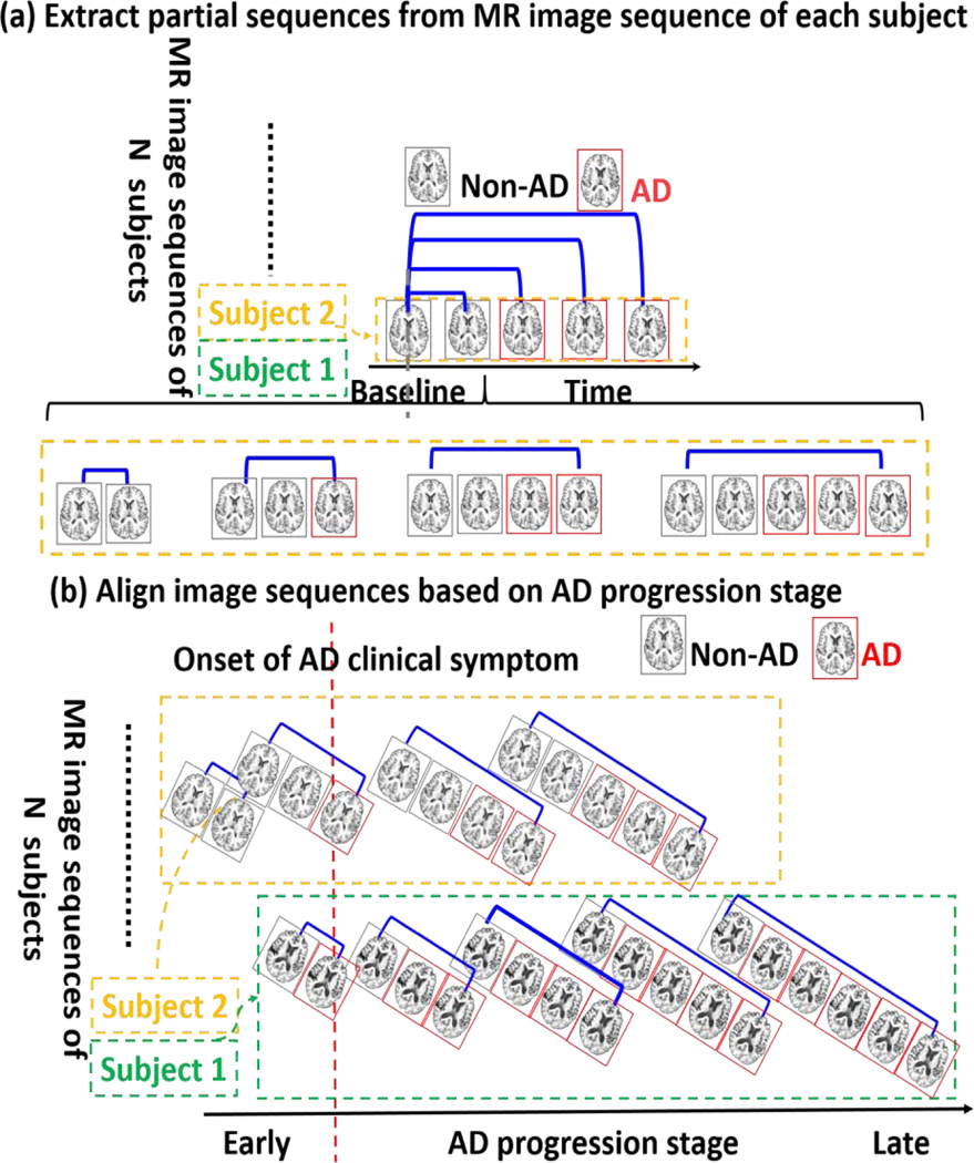
In order to train a classifier which is able to recognize different number of MR images collected at different AD progression stage, we will extract different length partial sequences to cover different AD progression stage for each subject. We can decompose the complete longitudinal image sequence into of partial image sequences where each is the partial image sequence with time points from baseline to follow-up as shown in Fig. 1. (a). Of note, all partial image sequences extracted from the same complete sequence use the same label. For each , we further extract longitudinal feature representations as . For each , we further extract longitudinal feature representations as , where the first column vector is are the average of morphological features from baseline to last time point and the second column vector measures the longitudinal difference of morphological features from baseline to the last follow-up inside the partial image sequence. It is apparent that each feature representation describes both the spatial and temporal morphological patterns. As we will explain in Section 3.4, feature selection is of necessity to remove data redundancy from such high dimensionality (). It is worth noting that the partial sequence refers to variable number of consecutive follow up MRIs and did not consider necessarily missing MRIs or variable time sampling of the follow up MRIs. In our experiment, we only selected all subjects follow up MRI scans every 6 months from ADNI dataset.
Fig. 1.
Prepare the training dataset. (a) We extract partial sequences of different length (from baseline to follow-ups, ) for each subject. (b) We align the extracted partial MR image sequences of each subject based on the AD progression stage before training TS-SVM.
B. Train Partial Sequences Using Classic SVM Model
We divide all morphological features extracted from the partial image sequences into two groups: positive sample set for MCI-C subjects and negative sample set for MCI-NC subjects. To recognize the longitudinal patterns involved in AD conversion, the naive way is to train a SVM by:
| (1) |
Where is a linear detection score function, is the support weight vector for separating MCI-C group and MCI-NC group, is the bias term to normalize the data distribution to zero mean, is a scalar balancing the regularization term and loss term, is the slack variable which compensates for the classification errors. The intuition behind two constraints in Eq. (1) is that the detection score for morphological pattern from each MCI-C subject is encouraged to be greater than 1 while the detection score for morphological pattern from MCI-NC subject is smaller than −1. Therefore, the MCI-C and MCI-NC groups are separated with a minimal margin of . In order to make the optimization adaptive to data distribution, we go one step further to jointly estimate the support vector , slack variable , and the bias term .
C. Long Range Early Diagnosis by Temporal Structured SVM
It is clear that there are strong temporal structural correlations along partial image sequences in each subject. However, the naive SVM solution shown in Eq. (1) treats each partial sequence equally and completely ignores the structural correlations. Thus, it is inevitable to have unrealistic inconsistent detection scores for MCI-C subject in the AD progression, although the structural change and AD progression are normally regarded as nonreversible. To alleviate this problem in the classic SVM method, we propose the following temporal structured-SVM method to achieve long range early diagnosis by leveraging the monotonicity of AD conversion risk, as described below.
Align spatial-temporal feature representations based on AD progression stage.
The partial image sequences extracted from each MCI-C subject cover different periods of AD progression which have different impact in recognizing the onset of AD symptom. To that end, we consider such impact is related with the AD progression stage for subject . Specifically, is defined by (1) determining the actual time point of AD conversion in each MCI-C subject (the first time point that the MCI-C subject has been clinically diagnosed as AD, shown by the red line in Fig. 1(b) tracing backward or forward to the last time point in each partial image sequence such that the time offset toward the time point of AD conversion indicates the progression stage . Specifically, represents the exact time point diagnosed as AD. Negative stage degree denotes the time period prior to AD conversion and the positive stage value represents the time period after AD converting. We treat all partial sequences from MCI-NC subjects equally in the training stage just as conventional SVM method since the actual AD converting time is unknown yet.
Temporally Structured Support Vector Machine.
After we associate the positive training samples with AD progression stage and align them based on subject-specific AD convert time, the energy function of our TS-SVM is defined as:
| (2) |
Where , are the AD progression stage parameters for partial sequences and from subject . denotes the margin parameter which reflect detection score temporal changes between different partial sequences and . can be any arbitrary non-negative function, and in general, it should be a non-decreasing function in (0,1]. For simplicity, we use the following linear function:
| (3) |
where is the maximum value of in all training data and is the minimum value of in all training data. Compared to the classic SVM in Eq. (1), our TS-SVM treats the partial sequences and adaptive to the AD progression. The detection score is constrained to be higher than by a margin . As a result, the detection score is constrained to increase monotonically with the AD progression stage for each subject as shown in Fig. 1 (b). We treat partial image sequences from MCI-C and MCI-NC groups differently in training stage. Specifically, we keep using the same set of morphological features of MCI-NC group as negative training samples. However, we did not apply the temporal consistency constraints on the MCI-NC subjects since we do not have enough information on the AD progression of those MCI-NC subjects. Therefore, we treat those partial sequences from MCI-NC subjects equally just as classic SVM. It is worth noting that such monotonicity constraint is only used in the training stage to seek for the more reasonable hyperplanes in support vector machine. In the testing stage, we apply the same TS-SVM to unseen image sequences and predict the risk of AD conversion.
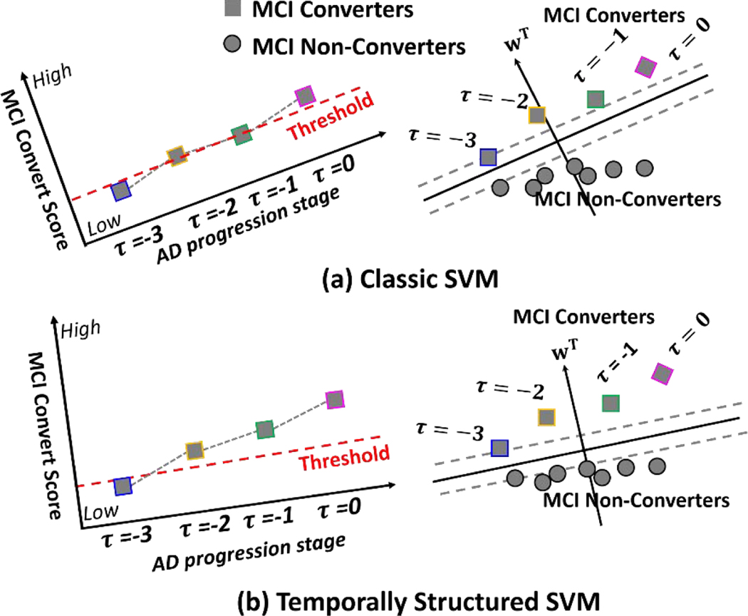
The benefit of our TS-SVM in AD early detection is illustrated in Fig. 2. Given the morphological features extracted from the partial image sequences, classic SVM trains the partial sequences at different AD progression stage equally, which leads to inconsistent detection score along with the AD progression as shown in Fig. 2 (a). On the contrary, our TS-SVM can leverage a sequence of monotonically increasing detection scores on positive samples to guide the optimization detection score function such that the detection scores with each MCI-C subject can consistently increase as AD pathology progresses as shown in Fig. 2 (b). As an additional heuristics, the monotonicity constraint eventually enhance the capability of early AD detection. Our TS-SVM is able to find a better hyper-plane which assign higher detection score for MCI converters at early stage. Therefore, our method is more sensitive to early AD onset.
Fig. 2.
Comparison of classic SVM and our temporal structured-SVM. The classic SVM treats each partial image sequences equally, even from the same subject. Since no temporal constraint is used in training classic SVM, the detection scores of classical SVM for MR image sequence are inconsistent along time as shown in (a). Our TS-SVM measures the impact of each partial image sequence based on the AD progression stage. Since our TS-SVM fully utilizes temporal consistency heuristics, the detection score of TS-SVM for MR image sequence is much more consistent than classic SVM as shown in (b).
D. Joint Feature Selection for Early AD Diagnosis
Since the morphological features are in high dimension, feature selection is a standard procedure to remove the data redundancy (Xiaofeng Zhu et al., 2020; X. Zhu et al., 2017; Y. Zhu et al., 2014; Y. Zhu et al., 2016; Y. Zhu et al., 2019). Usually feature selection is independently applied prior to train the classifiers. In order to make the selected best features eventually optimal for using TS-SVM, we proposed to jointly select best features and train the classifiers by further introducing a norm for group-wise sparsity on the classification vector :
| (4) |
where the group-wise sparsity constraint on selects a small number of features which are effective to suppress noisy patterns and reduce redundancy. Here the group sparsity strategy constrains that each ROI is either selected or discarded for all feature measurements (GM, WM, CSF, Background and Jacobian value). The learned can be regarded as both a classifier for classification and a coefficient matrix for supervised feature selection because, first, norm minimizes the energy for , so that the classification margin is maximized; secondly, norm selects discriminative ROIs separating MCI-C and MCI-NC groups to remove the redundant features. Therefore, our TS-SVM model turns into a simultaneous supervised feature selection and classification scenario.
E. Optimization
Although Equation (4) is a convex problem, it is hard to optimize it directly due to a large number of linear inequality constraints. To solve this problem efficiently, we reformulate it as an unconstrained problem which falls into the framework of Alternating Direction Method of Multipliers (ADMM) (Boyd et al., 2011a, 2011b; Nie et al., 2014).
F. Long Range Early Detection of AD on Longitudinal Image Sequence
In the application stage, we assume subjects keep taking the longitudinal MR image scans. For each subject, we can apply the learned TS-SVM after the first follow-up scan. At each time point, our AD detection/prediction process consists of two main steps, (1) estimate the AD conversion score using currently all available longitudinal information, and (2) analyze the risk of AD based on the historical prediction scores. The detail of each step is given below.
Step 1. Estimate the AD convert score. Suppose that the longitudinal image sequence currently has longitudinal scans so far. The estimation of AD convert score consists of two steps: (1.a) Extract the longitudinal features from longitudinal image sequence ; (1.b) Compute the AD convert score by letting .
Step 2. Analyze AD risk and early alarm of AD conversion. There are two criteria to trigger the alarm of AD convert: (1) the AD convert score is higher than 1, i.e., ; and (2) the increase of from previous AD convert score (using ) to current AD convert score is greater than another threshold , i.e., . We label the test subject as MCI-C cohort only if the trajectory of AD convert scores matches both two above criteria. Otherwise, we record the current AD convert score and wait for the future MR scan. It is worth noting that the threshold can be learned on a validation fold (completely separate from both training and testing dataset) by exhaustive search.
III. Experiments
A. Subject Information
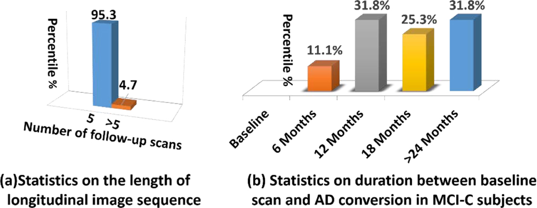
In this paper, 151 subjects in total are selected from ADNI dataset for performance evaluation, which consists of 70 MCI-C and 81 MCI-NC subjects. Detailed demographic information is summarized in Table 1. Based on the statistics of phenotype data (e.g., Mini-Mental State Examination (MMSE) score), it is clear that the phenotype data is not sufficient to distinguish MCI-C and MCI-NC subjects. MMSE is a clinical score used broadly in clinical and research to measure cognitive impairment. The range of MMSE is 0 to 30. The cutting off point of MMSE for AD is <25, MCI is 25–27, normal control is 28–30. Among all longitudinal subjects, the distribution of the number of longitudinal scans is shown in Fig. 3 (a) where most of subjects have at least 5 follow-up scans (excluding baseline scan). Specifically, we further inspect the duration between baseline scan and AD conversion in 70 MCI-C subjects. As shown in Fig. 3 (b), the AD convert occurs randomly after the baseline scan in our MCI-C training subjects.
Table 1.
Demographic information of the MCI-C and MCI-NC subjects.
| Female/Male | Age | MMSE | |||
|---|---|---|---|---|---|
| MCI-NC | 56/25 | 75.93±6.41 | 26.67± 3.69 | ||
| MCI-C | 52/18 | 74.70±4.75 | Before diag. | diagnosed | After diag. |
| 26.57±2.86 | 26.71±3.14 | 26.85±4.26 | |||
Fig. 3.
The distribution of the longitudinal MR image sequences for MCI-NC and MCI-C subjects in our dataset.
B. Image Processing
We downloaded raw digital imaging and communications in medicine (DICOM) MRI scans from the ADNI website http://www.adni-info.org/. All MR images have been reviewed for quality, and automatically corrected for spatial distortion caused by gradient nonlinearity and bias field inhomogeneity. The data are 1.5 T MRI data and all from ADNI1.
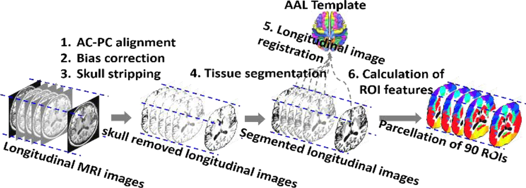
As displayed in Fig. 4, image processing was conducted by the following steps:
Fig. 4.
The images pre-processing and feature extraction step
Anterior commissure-posterior commissure correction using MIPAV software for all images;
Correct intensity inhomogeneity using N4 bias correction algorithm (Tustison et al., 2010);
Extract brain using a robust skull-stripping method (Fennema-Notestine et al., 2006);
Image segmentation by using the FAST program in FSL package (Zhang et al., 2001) to obtain the whole brain tissue segmentation of GM,WM, and CSF;
Parcellate whole image into 90 regions of interest (ROIs) by registering the AAL template (Kabani et al., 1998) (with manually labeled 90 ROIs) to each longitudinal image sequence via a longitudinal image registration method (Wu et al., 2012);
Calculate the tissue percentages of the GM, WM, CSF, background and the mean Jacobian values of displacements (estimated in Step 5) for each ROI.
C. Experiments Setup
Counterpart methods under comparison.
We compare our proposed TS-SVM based early detection method with classic SVM which is referred as SVM in the following experiments. Furthermore, we evaluate the impact of feature selection in both classic SVM and our TS-SVM, which are referred as SVM+FS and TS-SVM+FS, respectively. We use two types of data for the classic SVM method with feature selection penalty. Firstly, we apply single MR images to classic SVM with joint feature selection (denoted as SVM-S & SVM-S+FS); then, the novel extracted partial sequences are applied to SVM and joint feature selection (denoted as SVM-P & SVM-P+FS). It is worth noting that the partial sequences enables the classic SVM model be trained for different MR images automatically. Therefore, the early detection performance of classic SVM model using partial MR image sequences are improved a lot compared with using multiple MR images because it is trained for recognizing small partial sequences from different AD progression stage. Furthermore, we also selected a dataset with the partial sequences extracted from baseline to the early detection time scans by our TS-SVM method. We use this dataset to train classic SVM model with feature selection (denoted as SVM-EP & SVM-EP+FS). This is to evaluate the importance of the earliest detection time scans for classic SVM model.
Evaluation measurements.
We use several quantitative measurements to evaluate not only the classification accuracy but also the early detection range AD conversion. Besides the widely used Accuracy (ACC), Sensitivity (SEN) and Specificity (SPEC), we also employ F1-score which is defined as the harmonic mean of precision and recall values (Hoai et al., 2011; Hoai & Torre, 2014; Huang et al., 2014):
Where and , represents the number of accurately detected positive samples (MCI-C), represents the number of positive samples which are not detected, represents the number of negatives which are classified correctly and represents the number of negative samples which are not assigned with correct labels by our classifier. Of note, high indicates not only better performance in AD early detection but also the Precision and Recall are well balanced. We report the F1-score of our method compared with competing methods with respect to early detection time in order to show all competing methods dynamically.
Parameter selection.
We used ten-fold cross-validation strategy to evaluate the classification performance. In all experiments, we split the data into 10 non-overlap folds, where one fold is used as the testing data and the remaining nine folds are used for training at each time. We repeat the whole process for ten times to avoid any possible bias caused by dataset partition. The final classification accuracy is reported by averaging the classification results from cross validations. To learn the best parameters, we use five-fold inner cross validation strategy. We spilt the training data into five non overlap folds and use one fold data as the parameter validation data. The parameters are tuned using grid search strategy in the validation dataset (completely separated from testing dataset and training dataset).
D. Performance Evaluation on AD Early Detection
In each cross validation case, we train our TS-SVM on the training data and sequentially apply the trained classifier to the testing subject image sequence after the first follow-up. Since the month of converting to AD after baseline scans varies across MCI-C subjects, we show the detection Accuracy (ACC) and Accuracy Under ROC curve (AUC) for MCI-C subjects converting to AD in 18 months, 24 months, and 30 months after the baseline scan in Table 2, Table 3 and Table 4, respectively. It is clear that the SVM-P (partial MR images sequences) achieves highest accuracy compared to SVM-S (single MR images) and SVM-EP (earliest partial MR image sequences by TS-SVM). The partial sequences enable the SVM-P to recognize dynamic structure changes at any scanning time or AD progression stage. Therefore, SVM-P is more sensitive to different dynamic structure changes involved in AD progress. Our TS-SVM outperforms the SVM-P with more than 10% improvement in terms of ACC, which suggests the advantage of using temporal consistency and monotony constraints in our proposed method. Also, feature selection is very important to improve the detection accuracy. In average, our full method (TS-SVM+FS) can detect AD 6 months earlier than clinical diagnosis with 86.76% accuracy, 12 months earlier than clinical diagnosis with 82.5% accuracy, and 18 months earlier than clinical diagnosis with 76.53% accuracy.
Table 2.
Accuracy of AD detection at 6 and 0 months earlier than AD clinical diagnosis for the MCI-C subjects who converted to AD in 18 months after baseline scan.
| Method | 18 Earlier |
Months | 12 Earlier |
Month | 6 Earlier |
Months | 0 Earlier |
Months |
|---|---|---|---|---|---|---|---|---|
| AC C |
AU C |
AC C |
AU C |
AC C |
AU C |
AC C |
AU C |
|
| SVM-S | - | - | - | - | 0.6 653 | 0.7 153 | 0.6 826 | 0.7 241 |
|
SVM-
S+FS |
0.6 713 | 0.7 175 | 0.6 943 | 0.7 382 | ||||
| SVM-EP | - | - | - | - | 0.6 821 | 0.7 336 | 0.6 924 | 0.7 315 |
|
SVM-
EP+FS |
0.6 961 | 0.7 452 | 0.7 065 | 0.7 482 | ||||
| SVM-P | 0.7 110 | 0.7 612 | 0.7 345 | 0.7 937 | ||||
|
SVM-
P+FS |
- | - | - | - | 0.7 557 | 0.7 862 | 0.7 735 | 0.8 237 |
| TS-SVM | - | - | - | - | 0.8 816 | 0.9 327 | 0.8 975 | 0.9 431 |
|
TS-
SVM+FS |
- | - | - | - | 0.9 025 | 0.9 649 | 0.9 075 | 0.9 776 |
Table 3.
Accuracy of AD detection at 12, 6 and 0 months earlier than AD clinical diagnosis for the MCI-C subjects who converted to AD in 24 months after baseline scan.
| Method | 18 Earlier |
Months | 12 Earlier |
Month | 6 Earlier |
Months | 0 Earlier |
Months |
| AC C |
AU C |
AC C |
AU C |
AC C |
AU C |
AC C |
AU C |
|
| SVM-S | - | - | 0.6 285 | 0.6 634 | 0.6 324 | 0.6 782 | 0.6 805 | 0.7 215 |
|
SVM-
S+FS |
0.6 325 | 0.6 702 | 0.6 573 | 0.6 923 | 0.6 951 | 0.7 411 | ||
| SVM-EP | - | - | 0.6 452 | 0.6 837 | 0.6 612 | 0.7 024 | 0.6 923 | 0.7 351 |
|
SVM-
EP+FS |
0.6 535 | 0.6 921 | 0.6 761 | 0.7 155 | 0.6 987 | 0.7 438 | ||
| SVM-P | - | - | 0.7 325 | 0.7 822 | 0.7 455 | 0.7 917 | 0.7 535 | 0.8 223 |
|
SVM-
P+FS |
- | - | 0.7 537 | 0.7 912 | 0.7 685 | 0.8 123 | 0.7 725 | 0.8 314 |
| TS-SVM | - | - | 0.8 425 | 0.8 851 | 0.8 593 | 0.9 042 | 0.8 635 | 0.9 128 |
|
TS-
SVM+FS |
- | - | 0.8 475 | 0.8 932 | 0.8 720 | 0.9 277 | 0.8 812 | 0.9 216 |
Table 4.
Accuracy of AD detection at 18, 12, 6 and 0 months earlier than AD clinical diagnosis for the MCI-C subjects who converted to AD in 30 months after baseline scan.
| Method | 18 Earlier |
Months | 12 Earlier |
Month | 6 Earlier |
Months | 0 Earlier |
Months |
|---|---|---|---|---|---|---|---|---|
| AC C |
AU C |
AC C |
AU C |
AC C |
AU C |
AC C |
AU C |
|
| SVM-S | 0.5 534 |
0.5 913 |
0.5 541 |
0.5 953 |
0.5 954 |
0.6 315 |
0.6 152 |
0.6 551 |
|
SVM-
S+FS |
0.5 672 |
0.6 127 |
0.5 723 |
0.6 157 |
0.6 053 |
0.6 421 |
0.6 356 |
0.6 735 |
| SVM-EP | 0.5 623 |
0.6 034 |
0.5 716 |
0.6 125 |
0.6 039 |
0.6 452 |
0.6 241 |
0.6 645 |
|
SVM-
EP+FS |
0.5 742 |
0.6 151 |
0.5 821 |
0.6 261 |
0.6 145 |
0.6 603 |
0.6 365 |
0.6 803 |
| SVM-P | 0.6 016 |
0.6 542 |
0.6 025 |
0.6 677 |
0.6 325 |
0.6 712 |
0.6 515 |
0.6 931 |
|
SVM-
P+FS |
0.6 557 |
0.6 862 |
0.6 735 |
0.6 127 |
0.6 675 |
0.6 983 |
0.6 464 |
0.6 926 |
| TS-SVM | 0.7 345 |
0.7 734 |
0.7 675 |
0.8 116 |
0.7 805 |
0.8 334 |
0.7 875 |
0.8 503 |
|
TS-
SVM+FS |
0.7
653 |
0.7
983 |
0.8
125 |
0.8
434 |
0.8
345 |
0.8
672 |
0.8
431 |
0.8
894 |
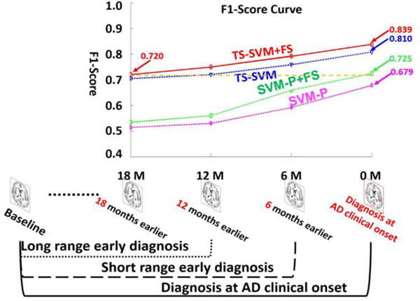
Furthermore, Fig. 5 shows the F1-scores in long-range early detection, short-range early detection, and AD diagnosis applications by four AD early detection competing methods: SVM-P, SVM-P+FS, TS-SVM, TS-SVM+FS. We only show the performance of SVM-P since it achieves best performance among the above competing methods using classic SVM. As displayed in the bottom of Fig. 5, AD diagnosis at clinical onset uses the longest longitudinal image sequence (baseline to clinical diagnosis time). In this scenario, our method can be used to provide imaging-based validation in clinical practice. On the contrary, long-range early diagnosis uses shortest longitudinal image sequence and detect early AD onset 12 months or 18 months earlier than the clinical diagnosis time. The accuracy of long-range early diagnosis is lower than short range early detection since less longitudinal images are used. However, our AD early detection method (TS-SVM+FS) can achieve F1-score = 0.720 18 months prior to clinical diagnosis time. This is comparable to the performance of classic SVM-P+FS at AD clinical diagnosis time (F1-socre = 0.725).
Fig. 5.
Averaged F1-score in AD diagnosis, short-range early diagnosis, and long-range early diagnosis by SVM-P (Magenta) and SVM-P+FS (green), our TS-SVM (blue) and our full method TS-SVM+FS (red). The SVM-P+FS (green) achieves best performance for classic SVM models.
Discussion.
We found that high detection performance is achieved in detecting AD 6–12 months prior to AD conversion time, but the performance drops dramatically in detecting AD for longer periods prior to AD conversion time. One explanation for this decrement in detection performance is bias inherent in the longitudinal data we used. In this dataset, for subjects that converted to AD after 6–12 months from the baseline scan, we have 2 or 3 follow up time points, therefore, there were enough follow ups in the training data for the detector. However, for MCI subjects that converted to AD 18 months from the baseline scan, there was only one follow up. Due to the lack of follow-up data points for these subjects, the training data is severely biased. We believe that if enough follow-ups are provided for subjects that convert to AD after 18 months since the baseline scan, the performance of TS-SVM will improve.
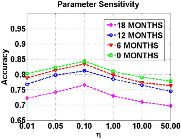
In our full method (TS-SVM+FS), there is only one regularization parameter (Eq. (3)) which balances the sparsity of the learned support vector and the inequality constraints. It is worth noting that other important parameters such as adaptive margin and training classification error are optimized in the training stage. Here we evaluate the sensitivity of parameter in AD early detection. Specifically, we set the value for from 0.01 to 50.0 and evaluate the classification accuracy on the validation dataset. Fig. 6 shows the detection accuracy vs. the value of parameter with different detection ranges. It is straightforward to determine the optimal parameter which is very consistent in either short term or long term early detection applications.
Fig. 6.
The valuation of parameter sensitivity for variable which balances the sparsity constraint and inequality constraints in Eq. (4).
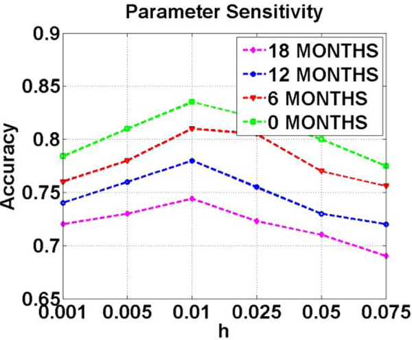
Another important parameter related to temporal dynamics in AD progression is h. A large value of h indicates individual is developing from MCI/NC to AD quickly. It is especially important for early AD diagnosis. We set the optimal value for h based on an independent validation dataset. We show the detection accuracy vs. the value of parameter in Fig. 7 computed on our validation dataset. The optimal value for in our experiments is set to be 0.01.
Fig. 7.
The valuation of parameter sensitivity for variable for evaluate the monotonicity of testing subjects.
Convergence analysis.
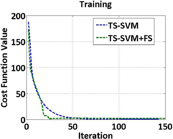
We display the averaged convergence curve on the ten cross validation folds of training dataset. All the parameters involved are fixed using the best value obtained by grid search. Fig. 8 shows the convergence curves by TS-SVM and TS-SVM+FS methods. It can be seen that the value of objective functions (Eq. (2) by TS-SVM and Eq. (3) by TS-SVM+FS) converges after 100 iterations for both methods.
Fig. 8.
The cost function values vs. iteration numbers by TS-SVM and TS-SVM+FS methods.
E. Depict Critical Brain Regions Intensively Involved in AD Progression
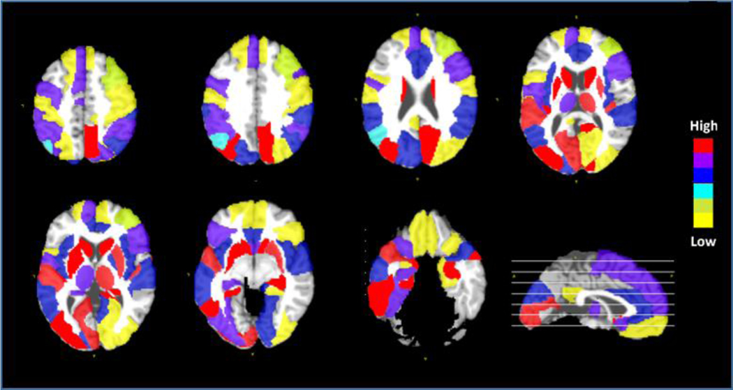
Since our method jointly selects morphological features during training TS-SVM, it is possible to visualize the predictive impact of each brain region by examining the contribution of morphological features computed from each ROI in our early AD detection method. Intuitively, the higher the overall weight of the morphological patterns extracted from a particular brain region, the greater role this region has in predicting AD conversion. In Fig. 9, we visualized the top 20 brain regions with largest overall weights after feature selection, which are strongly associated with AD progression. The brain regions highlighted include neocortical and paralimbic areas (medial/lateral temporal lobe, medial/lateral parietal lobe, and occipito-frontal cortex) that are selectively affected in AD. A few subcortical regions including the hippocampus, caudate nucleus, putamen, and thalamus were also implicated to predict conversion to AD, likely reflecting striato-thalamic nodes in cortical-subcortical functional networks (Hoesen et al., 2000; S. Risacher & A. Saykin, 2013; S. L. Risacher & A. J. Saykin, 2013).
Fig. 9.
The top 20 selected ROIs by the proposed TS-SVM+FS method which are highly involved in early detection of AD progression. We repeat ten In each test, we select top 20 ROIs. This figure shows the frequency of ROIs selected in those ten-fold cross validation. Different color indicates different selection frequency.
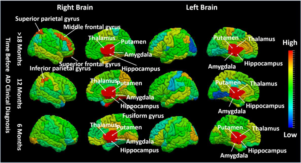
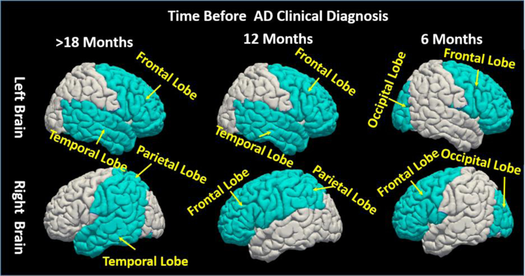
Furthermore, we separate the training image sequences into three AD conversion groups based on the time course of progression: Group 1 (conversion to AD 12 months post-baseline), Group 2 (conversion to AD 18 months post-baseline, and Group 3 (conversion to AD > 24 months post-baseline). For each group, we apply our TS-SVM+FS method separately. The goal of this experiment is to investigate the association of each brain region to AD progression. We map the contribution of each anatomical region onto the brain surface displayed in Fig. 10, where red and blue denote a strong or weak relationship to AD conversion, respectively. Of note, the significance score in each region is measured by the normalized feature selection weights of all morphological patterns extracted from the underlying region. It is clear that (1) some subcortical regions such as hippocampus, putamen, amygdala, and thalamus are always active during AD progression; (2) left and right cerebral hemispheres are differentially associated with AD progression. Due to the limited number of training samples in each group, it is difficult to interpret the feature selection results for each brain region in the cortical area. Instead, we examine the impacts of L/R frontal lobe, L/R parietal lobe, L/R temporal lobe, and L/R occipital lobe, respectively. We display the most active lobe in Fig. 11, the selected top four lobes are colored by light blue and other regions are colored by gray. As displayed in Fig. 11, it is clear that selective temporal lobe changes are the primary locus associated with earlier AD conversion, whereas the occipital lobe is relatively spared in early AD converters. However, over longer observation periods (>12 months), the relative weights of temporal and occipital lobe involvement in conversion to AD begin to converge.
Fig. 10.
Visualization of impacts of each brain region in AD progression. We color-code all ROIs by their respective selected frequency in our experiments at different AD progression stage: 18 Months, 12 Months and 6 Months before AD conversion. (red: high impact; blue: low impact).
Fig. 11.
Visualization of impacts of each brain lobe in AD progression. The light blue colored lobes are the top selected lobes. We show the top four selected lobes at different AD progression stage. At the early AD progression stage (18 Months before converting to AD) the temporal lobes, partial lobe and the frontal lobe are selected; The occipital lobe and the temporal lobe are selected at the late AD progression stage (i.e. 6 Months before convert to AD).
Discussion.
Our novel analytical method robustly detects AD at time points 6 or 12 months prior to conversion from MCI. By contrast, performance for predicting conversion drops markedly at 18 months. One reason for this drop-off in performance is an inherent bias in the ADNI dataset. Whereas subjects converting to AD at 12 or 18 months from baseline had three or four follow-up scans, the majority of MCI subjects that converted to AD 24 months out from baseline scan had only one subsequent scan. This difference in available training data imposes a significant limitation. We believe that the performance of our TS-SVM can be improved by having data from more time points. Our current work only uses single-modality data to classify MCI converters from MCI non-converters with accuracy > 80% using two MR images. We believe that performance can be significantly improved if this model can be trained using multiple modality data. Furthermore, in real-world clinical applications, our method would have to account for more groups than just MCI converters and MCI non-converters, the binary classification approach used in this study. Future work will explore the multiple-class classification problem to make this method suitable for real clinical applications.
F. Performance Evaluation in the Real Clinic Setting
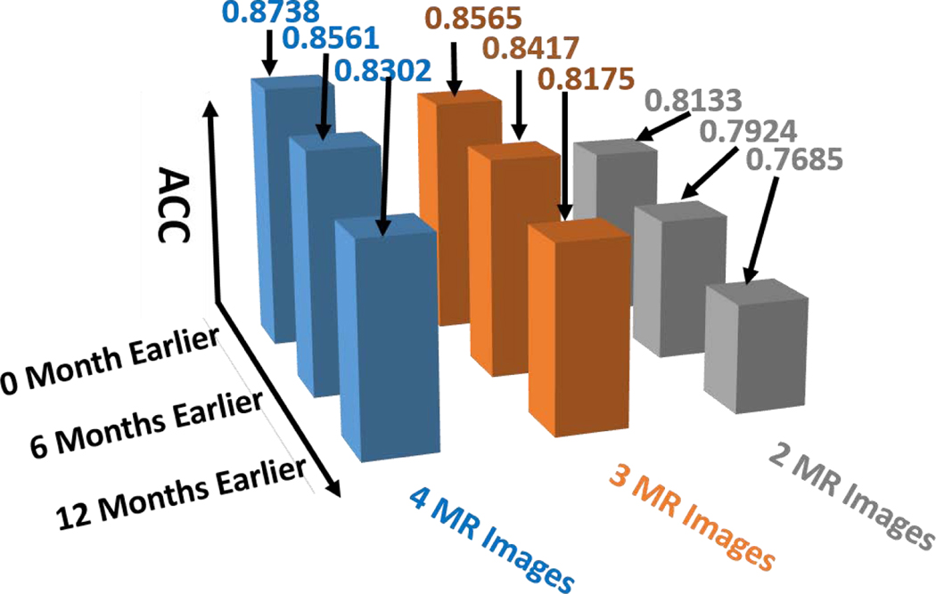
In the previous experiments, we do not consider the factor of number of MR scans used in early diagnosis, as show in Table 2–4. However, in general clinical practice, it is very different to have elderly people scanned more than three times, even on a yearly basis. Hence, we specifically report the prediction accuracy in terms of alarm window and number of MR images. As shown in Fig. 12, the prediction accuracy consistently increases when more longitudinal MR scans are used for prediction. Our early diagnosis method is able to predict AD conversion 12 months ahead of clinic diagnosis with 81.75% accuracy using just two follow-up MR scans, which indicates the realistic potential to apply our computer assisted early diagnosis method to the clinic arena.
Fig. 12.
The performance of AD early diagnosis in the real clinic setting where we use no more than three follow-up MR scans including baseline scan.
G. Performance Evaluation of Our Method with Demographic and Clinical Data Included
Although the focus of our work is to show that the temporal morphologic structure changes captured in longitudinal MR images are discriminative biomarkers for identifying the MCI subtypes: MCI converters vs. MCI non-converters, the AD risk factors in demographic data should not be ignored. Our model is very flexible to combine this demographic information to improve the performance. In this section, we add the AD risk factors including gender, education level, date of birth, APOE4 allele count (a gene which increases the risk for AD), APOE2 allele count ( a gene which enhances neuroprotection against AD) as the input feature of our model(Altmann et al., 2014; Chiang et al., 2010).Similarly, we use 10-fold cross-validation strategy and vary the available MR Images (2, 3, 4) for testing subjects. Table 5 shows the mean AD diagnosis accuracy with 0, 1 (baseline), 2, 3 and 4 MR images available at 0, 6, 12, 18, 24 months before clinical onset time. The demographic data increases the performance of our method substantially. For example, with 2 MR images, we can predict AD 12 month earlier at the accuracy of 87.2%, which increases about 10% compare to our model trained on MR images only. The improved model can predict AD 24 months earlier than clinical diagnosis time with accuracy of 83.1%.
Table 5.
Accuracy of AD diagnosis including gender, education, APOE 4, APOE2, age and baseline cognitive score (MMSE) by our method, at 24, 18, 12, 6 and 0 months earlier than AD clinical diagnosis for the MCI-C subjects with 0, 1, 2, 3 and 4 MR Images including baseline scan.
| Early Diagnosis Time | 4 Images |
MR | 3 Images |
MR | 2 Images |
MR | 1 Images |
MR | 0 Images |
MR |
|---|---|---|---|---|---|---|---|---|---|---|
| A CC |
A UC |
A CC |
A UC |
A CC |
A UC |
AC C |
AU C |
AC C |
AU C |
|
| 0 months earlier | 0.952 | 0.962 | 0.931 | 0.953 | 0.914 | 0.928 | 0.843 | 0.862 | 0.772 | 0.787 |
| 6 month earlier | 0.931 | 0.949 | 0.916 | 0.925 | 0.895 | 0.911 | 0.812 | 0.824 | 0.755 | 0.762 |
| 12 month earlier | 0.905 | 0.917 | 0.887 | 0.903 | 0.872 | 0.893 | 0.772 | 0.793 | 0.731 | 0.753 |
| 18 month earlier | 0.873 | 0.891 | 0.862 | 0.879 | 0.854 | 0.862 | 0.750 | 0.762 | 0.712 | 0.728 |
| 24 month earlier | 0.854 | 0.865 | 0.839 | 0.851 | 0.822 | 0.831 | 0.735 | 0.747 | 0.681 | 0.713 |
We added the results of our model using only the demographic data (gender, education, age) and genomics data: APOE2, APOE4 as one of our baseline model show in table 5 (0 MR Image). We also add the results on using only one baseline MR image along with all demographic data and APOE2, APOE4 as shown in table 5 (1 MR image). With only the demographic and gene data, our model shows accuracy at 68.1% to predict the AD 24 month earlier than clinical diagnosis time (drops about >4.5%) compared to using 1 MR image. With only baseline MR image, our model shows accuracy at 73.2% (decreased >8% compared to using 2 MRI scans) to predict AD 24 months before clinical diagnosis time.
This result in Table 5 demonstrated that the neuroimaging features are very important for the prediction of AD. It has been shown by neuroscientist that the brain structure starts to change from normal to abnormal first during the AD developing process (C. R. Jack, Jr. et al., 2010). The memory and cognitive ability starts to changes to abnormal after the brain structure changing. Since the neuroimaging data (MRI) can capture the brain morphological structures and clinical test only capture the cognitive and memory ability changes, the neuroimaging data will capture the early brain changes than cognitive test. Therefore, using neuroimaging data are more informative than cognitive test especially for early AD diagnosis. Furthermore, with two MRI scans compared to one MRI scan, our model shows a large improvement (>8%) on early AD prediction, which demonstrated that the longitudinal/temporal morphological structures measured by MRI scan is a crucial biomarker for successful AD prediction (early diagnosis).
Discussion.
This is an extended work of the paper (Y. Zhu et al., 2016)[40], we have extended the paper in several aspects: Firstly, we analysis the structural SVM with temporal monotonicity constraints with more details on F1 score of AD prediction at different time frame (18, 12, 6 months before clinical diagnosis time), optimization, parameter sensitivity and algorithm convergence. Secondly, we also added more detail information on the dataset such as the distribution of visiting number, disease status (NC, MCI converter, MCI non-converter and AD) and clinical scores. Thirdly, we add the demographic information and genetic data as the input of our model and show that it can consistently improve AD diagnosis and prediction performance. Fourthly, we analyzed the selected brain regions by our model in right and left brain at different time (6 months, 12 months and 18 months before clinical diagnosis time). At last, we discussed the scenario of applying this method in clinical practice and show the prediction accuracy at different disease stage (12, 6 and 0 months before clinical diagnosis) with different number (2, 3, 4) of longitudinal MRI scans available.
IV. Conclusion
In this paper, we present a novel method for predicting conversion from MCI to AD using a minimal number of MR images (2 MR images) based on a Temporally Structural-SVM (TS-SVM) and joint feature selection framework. In order to allow our model to accommodate fewer MR images during the testing process, we extract different length partial MR image sequences at different time points for each subject in the training data. Furthermore, to avoid inconsistent and unrealistic detection results, we enforce monotony on the output of SVM since AD progression is generally inexorable (Durrleman et al., 2009). In order to achieve early alarm of the onset of AD symptom, we propose to constrain the score of MCI converters to increase monotonically with AD progression (more follow-up scans are examined). Furthermore, we jointly perform feature selection and classification of TS-SVM, yielding promising results in terms of MCI-converters/MCI-Non-Converters classification accuracy using a lower number of MR images compared to the standard SVM approach.
Appendix – Optimization
Optimization:
Eq. (4) is a special case of convex problem with global minimum since the objective function is a semi-positive definite quadratic problem with linear constraints. However, it is hard to optimize Eq. (4) directly due to the large number of linear inequality constraints (several inequality constraints for each subject in the training data). To solve this problem efficiently, we introduce the hinge loss function to measure the error of inequality constraints (Hoai et al., 2011; Hoai & Torre, 2014; Huang et al., 2014), a dummy variable to separate the group sparsity constraint from other inequality constraints and use the Alternating Direction Method of Multipliers (ADMM) (Boyd et al., 2011a) to remove the inequality constraints. Now, we reformulate it as an unconstrained convex problem by rewriting Eq. (4) as,
| (5) |
where is a hinge loss function used to measure the error of inequality constraints with the quadratic loss: , is the penalty parameters for the constraint . and is the Lagrange Multiplier for the equality conraint .
Eq. (5) can be solved by alternatively updating the gradient of the overall energy function with respect to , , and until the overall energy function converges. The Lagrange parameters and the penalty parameter can be estimated in the iteration. At iteration, the Lagrange Multiplier and penalty parameter are updated as: , , where is a learning step parameter usually set to be slightly more than 1. In this way, the penalty value for equality constraint is increased gradually in each iteration. We set in our experiment.
Footnotes
Publisher's Disclaimer: This is a PDF file of an unedited manuscript that has been accepted for publication. As a service to our customers we are providing this early version of the manuscript. The manuscript will undergo copyediting, typesetting, and review of the resulting proof before it is published in its final form. Please note that during the production process errors may be discovered which could affect the content, and all legal disclaimers that apply to the journal pertain.
References
- Altmann A, et al. (2014). Sex modifies the APOE-related risk of developing Alzheimer disease. Ann Neurol, 75(4), 563–573. doi: 10.1002/ana.24135 [DOI] [PMC free article] [PubMed] [Google Scholar]
- Boyd S, et al. (2011a). Distributed Optimization and Statistical Learning via the Alternating Direction Method of Multipliers. Found. Trends Mach. Learn, 3(1), 1–122. doi: 10.1561/2200000016 [DOI] [Google Scholar]
- Boyd S, et al. (2011b). Distributed Optimization and Statistical Learning via the Alternating Direction Method of Multipliers. Foundations and Trends in Machine Learning, 3(1), 1–122. [Google Scholar]
- Chetelat G. a., & Baron J-C (2003). Early diagnosis of alzheimer’s disease: contribution of structural neuroimaging. NeuroImage, 18(2), 525–541. [DOI] [PubMed] [Google Scholar]
- Chiang GC, et al. (2010). Hippocampal atrophy rates and CSF biomarkers in elderly APOE2 normal subjects. Neurology, 75(22), 1976–1981. doi: 10.1212/WNL.0b013e3181ffe4d1 [DOI] [PMC free article] [PubMed] [Google Scholar]
- Chincarini A, et al. (2016). Integrating longitudinal information in hippocampal volume measurements for the early detection of Alzheimer’s disease. NeuroImage, 125(1), 834–847. [DOI] [PubMed] [Google Scholar]
- Cummings JL, et al. (2007). Disease-modifying therapies for Alzheimer disease: challenges to early intervention. Neurology, 69. doi: 10.1212/01.wnl.0000295996.54210.69 [DOI] [PubMed] [Google Scholar]
- Duchesne S, et al. (2008). MRI-Based Automated Computer Classification of Probable AD Versus Normal Controls. Medical Imaging, IEEE Transactions on, 27(4), 509–520. [DOI] [PubMed] [Google Scholar]
- Durrleman S, et al. (2009). Statistical models of sets of curves and surfaces based on currents. Medical Image Analysis, 13(5), 793–808. [DOI] [PubMed] [Google Scholar]
- Fennema-Notestine C, et al. (2006). Quantitative Evaluation of Automated Skull-Stripping Methods Applied to Contemporary and Legacy Images: Effects of Diagnosis, Bias Correction, and Slice Location. Human Brain Mapping, 27(2), 99–113. [DOI] [PMC free article] [PubMed] [Google Scholar]
- Filley C. (1995). Alzheimer’s disease: it’s irreversible but not untreatable. Geriatrics, 50(7), 18–23. [PubMed] [Google Scholar]
- Ganguli M, et al. (2010). Prevalence of mild cognitive impairment by multiple classifications: the Monongahela-Youghiogheny Healthy Aging Team (MYHAT) project. Am J Geriatr Psychiatry, 18. doi: 10.1097/JGP.0b013e3181cdee4f [DOI] [PMC free article] [PubMed] [Google Scholar]
- Ganguli M, et al. (2004). Mild cognitive impairment, amnestic type-An epidemiologic study. Neurology, 63(7), 115–121. [DOI] [PubMed] [Google Scholar]
- Gauthier SG (2005). Alzheimer’s disease: the benefits of early treatment. European Journal of Neurology, 12(3), 11–16. [DOI] [PubMed] [Google Scholar]
- Grimmer T, et al. (2009). Clinical severity of Alzheimer’s disease is associated with PIB uptake in PET. Neurobiol Aging, 30. doi: 10.1016/j.neurobiolaging.2008.01.016 [DOI] [PubMed] [Google Scholar]
- Hoai M, et al. (2011). Joint segmentation and classification of human actions in video. Paper presented at the Computer Vision and Pattern Recognition (CVPR), 2011 IEEE Conference on. [Google Scholar]
- Hoai M, & Torre F. (2014). Max-margin early event detectors. International Journal of Computer Vision, 107(2), 191–202. [Google Scholar]
- Hoesen GWV, et al. (2000). Orbitofrontal Cortex Pathology in Alzheimer’s Disease. Cerebral Cortex, 10(3), 243–251. [DOI] [PubMed] [Google Scholar]
- Hua X, et al. (2011). Accurate measurement of brain changes in longitudinal MRI scans using tensor-based morphometry. NeuroImage, 57(1), 5–14. [DOI] [PMC free article] [PubMed] [Google Scholar]
- Hua X, et al. (2010). Mapping Alzheimer’s disease progression in 1309 MRI scans: power estimates for different inter-scan intervals. NeuroImage, 51(1), 63–75. [DOI] [PMC free article] [PubMed] [Google Scholar]
- Huang D, et al. (2014). Sequential Max-Margin Event Detectors. Paper presented at the Computer Vision – ECCV 2014. [Google Scholar]
- Jack CR Jr., et al. (2010). Hypothetical model of dynamic biomarkers of the Alzheimer’s pathological cascade. Lancet Neurol, 9(1), 119–128. doi: 10.1016/s1474-4422(09)70299-6 [DOI] [PMC free article] [PubMed] [Google Scholar]
- Jack CR, et al. (2003). MRI as a biomarker of disease progression in a therapeutic trial of milame-line for AD. [DOI] [PMC free article] [PubMed]
- Johnson DK, et al. (2009). Longitudinal study of the transition from healthy aging to Alzheimer disease. Arch Neurol, 66. doi: 10.1001/archneurol.2009.158 [DOI] [PMC free article] [PubMed] [Google Scholar]
- Kabani N, et al. (1998). 3D anatomical atlas of the human brain. Paper presented at the Proc of HBM, NeuroImage. [Google Scholar]
- Klöppel S, et al. (2008). Automatic classification of MR scans in Alzheimer’s disease. Brain, 132(Pt 4), 681–690. [DOI] [PMC free article] [PubMed] [Google Scholar]
- Lam B, et al. (2013). Clinical, imaging, and pathological heterogeneity of the Alzheimer’s disease syndrome. Alzheimer’s Research & Therapy, 5(1). [DOI] [PMC free article] [PubMed] [Google Scholar]
- Lee E, et al. (2015). BFLCRM: A BAYESIAN FUNCTIONAL LINEAR COX REGRESSION MODEL FOR PREDICTING TIME TO CONVERSION TO ALZHEIMER’S DISEASE. The Annuals of Applied Statistics, 9(4), 2153–2178. [DOI] [PMC free article] [PubMed] [Google Scholar]
- Li Y, et al. (2012). Discriminant analysis of longitudinal cortical thickness changes in Alzheimer’s disease using dynamic and network features. Neurobiology of Aging, 33(2), 427.e415–430. [DOI] [PMC free article] [PubMed] [Google Scholar]
- Loewenstein DA, et al. (2006). Cognitive profiles in Alzheimer’s disease and in mild cognitive impairment of different etiologies. Dement Geriatr Cogn Disord, 21. doi: 10.1159/000091522 [DOI] [PubMed] [Google Scholar]
- Nie F, et al. (2014). New primal svm solver with linear computational cost for big data classifications Paper presented at the 31th International Conference on Machine Learning, Beijing, China. [Google Scholar]
- Petersen RC (2000). Mild cognitive impairment: transition between aging and Alzheimer’s disease. Neurologia, 15. [PubMed] [Google Scholar]
- Reisberg B, et al. (2008). Mild cognitive impairment (MCI): a historical perspective. International psychogeriatrics, 20(1), 18–31. [DOI] [PubMed] [Google Scholar]
- Risacher S, & Saykin A. (2013). Neuroimaging biomarkers of neurodegenerative diseases and dementia. Seminars in Neuroglgy, 33(4), 386–416. [DOI] [PMC free article] [PubMed] [Google Scholar]
- Risacher SL, & Saykin AJ (2013). Neuroimaging Biomarkers of Neurodegenerative Diseases and Dementia. Seminars in neurology, 33(4), 386–416. doi: 10.1055/s-0033-1359312 [DOI] [PMC free article] [PubMed] [Google Scholar]
- Shen D, & Davatzikos C. (2003). Very high-resolution morphometry using mass-preserving deformations and HAMMER elastic registration. NeuroImage, 18(1), 28–41. doi: 10.1006/nimg.2002.1301 [DOI] [PubMed] [Google Scholar]
- Thompson PM, et al. (2007). Tracking Alzheimer’s Disease. Annals of New York Academy of Sciences, 1097, 198–214. [DOI] [PMC free article] [PubMed] [Google Scholar]
- Tustison N, et al. (2010). N4ITK: improved N3 bias correction. IEEE Trans. on Medical Imaging, 29(6), 1310–1320. [DOI] [PMC free article] [PubMed] [Google Scholar]
- Vemuri P, et al. (2009). MRI and CSF biomarkers in normal, MCI, and AD subjects: diagnostic discrimination and cognitive correlations. Neurology, 73. doi: 10.1212/WNL.0b013e3181af79e5 [DOI] [PMC free article] [PubMed] [Google Scholar]
- Whitwell JL, et al. (2008). MRI patterns of atrophy associated with progression to AD in amnestic mild cognitive impairment. Neurology, 70. doi: 10.1212/01.wnl.0000280575.77437.a2 [DOI] [PMC free article] [PubMed] [Google Scholar]
- Winblad B, et al. (2004). Mild cognitive impairment - beyond controversies, towards a consensus: report of the International Working Group on Mild Cognitive Impairment. J Intern Med, 256. doi: 10.1111/j.13652796.2004.01380.x [DOI] [PubMed] [Google Scholar]
- Wu G, et al. (2012). Registration of longitudinal brain image sequences with implicit template and spatial-temporal heuristics. NeuroImage, 59(1), 404–421. [DOI] [PMC free article] [PubMed] [Google Scholar]
- Zhang Y, et al. (2001). Segmentation of brain MR images through a hidden Markov random field model and the expectation-maximization algorithm. IEEE Trans. on Medical Imaging, 20(1), 45–57. [DOI] [PubMed] [Google Scholar]
- Zhu X, et al. (2020). Spectral clustering via half-quadratic optimization. World Wide Web, 23(3), 1969–1988. doi: 10.1007/s11280-019-00731-8 [DOI] [Google Scholar]
- Zhu X, et al. (2017). Robust Joint Graph Sparse Coding for Unsupervised Spectral Feature Selection. IEEE Trans Neural Netw Learn Syst, 28(6), 1263–1275. doi: 10.1109/tnnls.2016.2521602 [DOI] [PubMed] [Google Scholar]
- Zhu Y, et al. (2014, 23–28 June 2014). Complex Non-rigid Motion 3D Reconstruction by Union of Subspaces. Paper presented at the 2014 IEEE Conference on Computer Vision and Pattern Recognition. [Google Scholar]
- Zhu Y, et al. (2016). Early Diagnosis of Alzheimer’s Disease by Joint Feature Selection and Classification on Temporally Structured Support Vector Machine. Med Image Comput Comput Assist Interv, 9900, 264–272. doi: 10.1007/978-3-319-46720-7_31 [DOI] [PMC free article] [PubMed] [Google Scholar]
- Zhu Y, et al. (2019). Dynamic Hyper-Graph Inference Framework for Computer-Assisted Diagnosis of Neurodegenerative Diseases. IEEE Trans Med Imaging, 38(2), 608–616. doi: 10.1109/tmi.2018.2868086 [DOI] [PMC free article] [PubMed] [Google Scholar]


