dcSBM: A federated constrained source‐based morphometry approach for multivariate brain structure mapping

Abstract

The examination of multivariate brain morphometry patterns has gained attention in recent years, especially for their powerful exploratory capabilities in the study of differences between patients and controls. Among the many existing methods and tools for the analysis of brain anatomy based on structural magnetic resonance imaging data, data‐driven source‐based morphometry (SBM) focuses on the exploratory detection of such patterns. Here, we implement a semi‐blind extension of SBM, called constrained source‐based morphometry (constrained SBM), which enables the extraction of maximally independent reference‐alike sources using the constrained independent component analysis (ICA) approach. To do this, we combine SBM with a set of reference components covering the full brain, derived from a large independent data set (UKBiobank), to provide a fully automated SBM framework. This also allows us to implement a federated version of constrained SBM (cSBM) to allow analysis of data that is not locally accessible. In our proposed decentralized constrained source‐based morphometry (dcSBM), the original data never leaves the local site. Each site operates constrained ICA on its private local data using a common distributed computation platform. Next, an aggregator/master node aggregates the results estimated from each local site and applies statistical analysis to estimate the significance of the sources. Finally, we utilize two additional multisite patient data sets to validate our model by comparing the resulting group difference estimates from both cSBM and dcSBM.

While centralized source‐based morphometry (SBM) is effective when data are locally accessible, it cannot operate on data that is decentralized. To address this limitation, we have introduced decentralized constrained source‐based morphometry (dcSBM) and our extensive analysis demonstrates that the proposed dcSBM can operate on decentralized data and achieve results that are almost identical to those of centralized SBM.

1. INTRODUCTION

Structural magnetic resonance imaging (sMRI) is a widely used neuroimaging technique that can be used to assess brain morphometry. A typical approach to extract brain structural changes is to segment the brain into regions of interest (ROIs) and compute the relationship of the volume of each ROI with the variables of interest. However, such an approach makes the assumption that the brain can be divided anatomically from the MRI data. Another approach, voxel‐based morphometry (VBM), is used to estimate voxel‐wise differences (Good et al., 2001). As a massively univariate approach, VBM reports voxel‐wise changes across the brain in the form of statistical maps. However, its univariate nature means it cannot extract information about the relationship among the voxels. Additionally, VBM estimates are limited to the specific predictive effect defined by the user/design. To capture inter‐voxel information, a multivariate approach would be preferred.

Source‐based morphometry (SBM) is a multivariate data‐driven approach introduced to automatically detect the whole‐brain structure by using information from voxels (Xu et al., 2009). The goal of SBM is to estimate maximally spatially independent sources (whole‐brain spatial maps) that covary among subjects and to compute potential individual subject or group differences based on the degree of expression of these sources. SBM utilizes the combined techniques of VBM preprocessing (spatial normalization, segmentation, and intensity correction) and independent component analysis (ICA) to extract maximally spatially independent sources and then uses statistical measures to identify sources of interest. Prior studies have shown that SBM can preserve the spatial correlation between different brain regions (Pearlson et al., 2015; Sui et al., 2012). Recently, SBM has been utilized to analyze different brain disorders (Gupta et al., 2019), including Parkinson's (Premi et al., 2017), bipolar and borderline personality disorders (Lapomarda et al., 2021), schizophrenia (SZ) and bipolar disorder (Sorella et al., 2019), as well as brain abnormalities in children with autism (Grecucci et al., 2016; Pappaianni et al., 2018).

Combining both ROI and data‐driven methodologies, another multivariate data‐driven approach was proposed, namely, constrained source‐based morphometry (cSBM) (Luo et al., 2012). cSBM leverages the full utility of SBM with the ROI information and also provides automatic correspondence between data sets. Unlike the fully blind nature of SBM, Constrained SBM uses component map templates derived from an independent data set to estimate ordered structural networks from a new data set in an entirely automated manner. The estimated structural networks can be further analyzed based on potential associations between their degree of expression over subjects and different variables of interest (e.g., age, gender, site, etc.). As in traditional SBM, this leads to fewer statistical tests. However, constrained SBM enables prior information to steer the decomposition and, thus, specific hypotheses to be investigated. The original cSBM approach was applied to constrain a single component using seed regions from the default mode network. However, cSBM can be extended to a more general approach. We do this, motivated by our fMRI Neuromark approach (Du et al., 2020), which extracts component maps from independent data, then applies all of these as constraints to implement a fully automated ICA approach. Here, we leverage a similar idea for cSBM, effectively a structural MRI extension of the Neuromark framework.

Both SBM and constrained SBM (cSBM) have been implemented on a common foundation, assuming that data are locally available while running the experiments. However, in neuroimaging studies, it is not always possible to pool all data sets in a centralized location. Additionally, coordinating data collection and sharing across different sites can be time‐consuming and expensive. Even with proper permission controls and data anonymization, recent studies have found a potential risk of revealing the identity of subjects with rare diseases (Sweeney, 2002; Sweeney et al., 2015). The ensuing inability to pool data sets from such sites will reduce statistical power, and it may not be possible to detect disease effects from a single site's low number of data samples. In recent years, considerable work has been focused on leveraging decentralized computation for neuroimaging analysis (Bostami et al., 2021; Plis et al., 2016; Rissman & Wagner, 2012; D. K. Saha et al., 2017; D. K. Saha, Calhoun, et al., 2022). Gazula et al. introduced a decentralized VBM approach and applied it to 2000 sMRI data sets from 14 different sites (Gazula et al., 2021), demonstrating the benefits of multiple variable analysis in a decentralized scenario. To overcome the inability of SBM and cSBM to operate on decentralized data sets, we introduce a novel method called decentralized constrained source‐based morphometry (dcSBM), which implements the sMRI Neuromark framework in a way that allows decentralized analysis. Our approach inherits multivariate properties from constrained SBM but operates ICA across data located at sites without moving the data. At the end of decentralized evaluation, we aggregate loading parameters and sources from different sites and further investigate the obtained results with comparisons and ensuing statistical analysis. We apply our approach brain‐wide to a large data set from SZ patients and controls, and we investigate the obtained results with comparisons and ensuing statistical analysis. Finally, we deploy the new algorithm within an open‐source tool called Collaborative Informatics and Neuroimaging Suite Toolkit for Anonymous Computation (COINSTAC) (Plis et al., 2016).

We make four main contributions in this paper. First, we propose the use of a brain‐wide spatially cSBM approach. Second, we derive a decentralized (federated) version of this algorithm and show that it gives results similar to those from a centralized approach. Third, we apply the approach to a large N data set from SZ patients and controls and demonstrate that the approach identifies significant changes in covarying structural networks that are consistent with what we expect. Finally, we deploy the new algorithm within an open‐source tool called COINSTAC. In this work, we first describe the data acquisition and preprocessing steps. Following that, we describe our dcSBM approach and evaluate its performance on real data sets. Here, we conducted a comparative analysis between centralized and decentralized results on the same data sets. We investigated the reliability of our proposed model using a sizeable subset of the large sample UK Biobank prospective study. Next, we utilized the Function Biomedical Informatics Research Network (fBIRN) (Du et al., 2020) and Center for Biomedical Research Excellence (COBRE) (Aine et al., 2017) structural MRI data sets to assess the clinical utility of this approach. This was done by evaluating the significance and effect sizes of the association between the identified loading parameters of each source and different variables of interest. This work builds on our proposed method (D. K. Saha, Silva, et al., 2022) and expands its application to clinical data sets, improving the statistical analysis of results and reliability assessments.

2. MATERIALS AND METHODS

2.1. Data acquisition and preprocessing

We begin with a description of the three data sets utilized in this work.

2.1.1. UK Biobank data set

We first leverage the UK Biobank, a large independent data set, to derive the SBM component templates. In the UK Biobank data set, sagittal orientation was used for the T1 structural MRI data. Following the previous measurements of population brain shape and size from (Mennes et al., 2014), the front side of the brain is tilted down by 16° regarding the anterior commissure—posterior commissure line. The T1‐weighted structural image comprises the following parameters: field‐of‐view: $208\times 256\times 256$ matrix, duration: $5$ min, resolution: $1\times 1\times 1$ mm³, 3D MPRAGE, sagittal, in‐plane acceleration iPAT = $2$, prescan‐normalize. The superior–inferior field‐of‐view is set to $256$ mm.

We selected $3000$ unaffected subjects for our experiments. The subject‐level T1‐weighted sMRI data were preprocessed using SPM121 and a Gaussian smoothing kernel comprising full width at half maximum (FWHM) = $10$ mm was applied to the data.

2.1.2. fBIRN data set

The fBIRN data sets were collected from seven different sites. The subjects from six sites were collected on a 3 T Siemens Tim Trio System, while a 3 T General Electric Discovery MR750 scanner was used for one of the sites. The T1‐weighted acquisition parameters are described in (Gupta et al., 2015).

The following subject inclusion criteria were applied to all subjects: head motion $\le 3°$ and $\le 3$ mm. After applying these criteria, 165 healthy controls (HCs) (average age: 37.04 ± 10.86; range: 19–59 years; 46/119: female/male) and 152 patients with SZs (average age: 38.77 ± 11.63; range: 18–62 years; 34/118: female/male) were selected. Both HCs and SZs were matched by age, gender, and mean framewise displacement (FD) to avoid introducing confounding effects (age: p = .1758; gender: s = .3912; mean FD: p = .9657). It was also ensured that (1) HCs do not have any past or current psychiatric illness based on SCID assessment or a first‐degree relative diagnosed with Axis‐I psychotic disorder, and (2) SZs were clinically stable at the time of scanning.

2.1.3. COBRE data set

The MRI images were collected on a single 3 T Siemens Trio scanner with a 12‐channel radio frequency coil. T1‐weighted high‐resolution structural images were acquired with a five‐echo MPRAGE sequence with TE = 1.64, 3.5, 5.36, 7.22, and 9.08 ms, TR = $2.53$ s, TI = $1.2$ s, flip angle = 7°, number of excitations = $1$, slice thickness = $1$ mm, field of view = $256$ mm, and resolution = $256\times 256$. As in fBIRN, we applied similar subject inclusion criteria to the COBRE data set, resulting in 82 HCs (average age: $38.09\pm 11.67$; range: 18–65 years; 22/60: female/male) and 66 SZs (average age: $37.79\pm 14.45$; range: 19–65 years; 9/57: female/male). HCs and SZs were also matched by age, gender, and mean FD (age: $p=.8874$; gender: $p=.0794$; mean FD: $p=.6475$).

For fBIRN and COBRE data sets, we preprocessed the sMRI data using SPM12. We segmented the structural images into six tissue compartments, including gray matter, white matter, and CSF, using modulated normalization, resulting in gray matter volume features. These were then smoothed by a Gaussian kernel comprising the FWHM = 6 mm.

2.2. Creation of whole‐brain SBM references

For the prior whole‐brain references, 30 replicable spatial references ($R$) were identified from separate group ICA results on two different sMRI data sets: (1) the genomics superstruct project and (2) the human connectome project. Each data set contains $3500$ unaffected subjects (Du et al., 2020). These spatial references were derived using group ICA and are collectively referred to as the Neuromark_v01_sMRI_low_30 template.

2.3. Spatially constrained ICA

ICA is a widely used approach in the biomedical domain (Calhoun et al., 2009; Rahaman et al., 2022; D. K. Saha et al., 2021; R. Saha, Saha, et al., 2022). In SBM of structural MRI data, ICA is applied to factorize the multi‐subject volume matrix $X$ into a mixing matrix $A$ and a source matrix $S$, such that $X=\mathit{AS}$ and the rows of $S$ are statistically independent of one another. The columns of the mixing matrix contain the subject‐specific expression levels of each source, while the rows of the source matrix contain the corresponding brain spatial maps. The ICA decomposition applies special filtering to handle noise and provides maximally spatially independent sources highlighting areas of inter‐subject covariation known as structural networks (Xu et al., 2009).

Constrained SBM, a structural MRI version of our Neuromark approach (Du et al., 2020), uses component map templates derived from an independent data set to estimate ordered structural networks from a new data set in an entirely automated manner. For the prior information, a reference matrix $R$ that contains the templates of interest is chosen. Then, a closeness measure $g_W\left(S,R\right)$ between an estimated signal $S=\mathit{WX}$ and the reference signal $R$ is defined to restrict the learning process (Lin et al., 2010; Lu & Rajapakse, 2005). The constrained ICA framework utilized here is formulated via the following augmented multi‐objective loss (Du & Fan, 2013):

$$\underset{W}{\max }a\cdot J_W\left(S\right)+\left(1-a\right)\cdot g_W\left(S,R\right)$$

where $J_W\left(S\right)$ denotes a normalized approximation of the negentropy of the estimated source $S$ (this is a standard contrast function for ICA), $g_W\left(S,R\right)=\mathbb{E}\left(S,R\right)$ is the Pearson correlation coefficient between $S$ and $R$, and $a$ is a hyperparameter (the default setting in the GIFT toolbox is $a=.5$).

2.4. Decentralized source‐based morphometry

To utilize the multivariate cSBM approach on a data set that is distributed over different local sites, we introduce dcSBM. In the centralized case, we have a data set $X={\left[x_1\dots ,x_N\right]}^{{\rm T}}$, where $x_i\in {\mathrm{ℝ}}^V$ is the $V$‐dimensional gray matter feature vector of the $i$th subject. Applying constrained SBM on this data set yields independent gray matter maps, which can be assessed for group differences. In a decentralized environment, there are $L$ sites in total, and each site $\mathrm{\ell }$ has a data set $D_{\mathrm{\ell }}=\left\{\left(x_i,z_i\right):i\in \left\{1,2,\dots ,N_{\mathrm{\ell }}\right\}\right\}$ from $N_{\mathrm{\ell }}$ subjects, where $z_i\in \mathrm{ℝ}$ expresses the predictor variables age, gender, diagnosis, and site from subject $i$. Here, each local site $\mathrm{\ell }$ operates constrained ICA separately on its local data $X$ and stores mixing ($A_{\mathrm{\ell }}$), and source matrices ($S_{\mathrm{\ell }}$) locally. Each column of the mixing matrix represents the loading parameters for a given component, which reflect the degree to which the component maps are expressed in each subject. Before running local ICA, each site receives the same public reference maps $R$, which contain the prior information about the sources of interest. The local constrained ICA applied to the local data matrix $X_{\mathrm{\ell }}$ is guided by a fast fixed‐point algorithm, which is included as part of the group ICA toolbox GIFT.2 Guided by the reference matrix $R$, the local source matrix $S$ and mixing matrix $A$ are obtained from the data matrix $X$.

For the mixing matrix $A$, the values in each column represent the contribution of each component to all subjects. Meanwhile, each row of the source matrix $S$ represents maximally spatially independent maps that specify areas of coherent variability among subjects. Following local site‐specific constrained ICA, a master node is used to concatenate the mixing matrices from each site utilizing a decentralized aggregation process. Moreover, solely for the purpose of assessing the quality of results obtained with our approach, the source matrices were also aggregated across sites. The flow diagram of our approach is shown in Figure 1.

FIGURE 1.

Flow diagram of decentralized constrained SBM. SBM, source‐based morphometry.

For comparison, we also operate constrained ICA in a centralized environment. In centralized experiments, we simply pool together the data from all sites and run a single constrained ICA. Following extraction of mixing, and source matrices, we compare the decentralized results, aiming to demonstrate that the decentralized results closely approximate the utopian results from the centralized case.

2.5. Statistical analysis

2.5.1. Pairwise correlation

In this analysis, we used the fBIRN and COBRE data sets. As we acquired the fBIRN data set from seven different sites, we consider each of them as an individual local site during dcSBM. We collected the COBRE data set from a single site and considered this as a single site during the computation. Altogether, eight different sites are participating in this analysis. After running constrained ICA on each local site separately, we concatenated the mixing matrix and aggregated the source matrix from each site using a common aggregator. To analyze the decentralized results, we also pooled all fBIRN and COBRE data sets together and evaluated constrained ICA in a centralized manner. Then, we evaluated the correlation between the i ^th column of the centralized loadings and the i ^th column of the decentralized loading parameters. Finally, we also computed the correlations between corresponding rows of the centralized and decentralized source matrices.

2.5.2. Linear regression

Like before, we use both the fBIRN and COBRE datasets for this analysis. Our aim is to conduct linear regression on the aggregate decentralized mixing matrices from the dcSBM model. The predictor matrix $Z$ has dimensions $465\times 10$, where the variables (columns) are age, gender, diagnosis, site, and interactions between gender and diagnosis, gender and age, diagnosis and age, age and site, diagnosis and site, and gender and site. Here, we used the aggregate loading parameters as our response variable. Finally, we fit our data matrix $Z$ to $A$ in a linear regression model. As we have $30$ loading parameter columns (dependent variables), we run our linear regression model $30$ times and store the results. For comparison, we also applied linear regression on the cSBM model.

We also computed the effect size of the independent variables for each dependent variable. In our analysis, we used loading parameters as the dependent variables and considered age, gender, diagnosis, sites, and possible interactions between them as the independent variables. We used the ANOVA Type 2 method to evaluate the effect size.

2.5.3. Model reliability

To examine the reliability of our proposed method, here we designed three different experiments using the UK Biobank data set. In the first experiment, we calculated the correlation, mean square error (MSE), max absolute error (MaxAE), and median absolute error (MedianAE) among the correlation matrices of loadings and sources separately. In the second experiment, we computed the correlation and MSE between the correlation matrices of loadings and sources separately. In the third experiment, we consistently increased the number of samples to analyze the performance of an effective federated environment.

1. Random shuffle

In this experiment, we artificially created three different sites, and $3000$ UK Biobank subjects were used to perform this experiment. In each experiment, we shuffled the subjects and assigned $1000$ distinct subjects to each site. We repeated this experiment 10 times and collected the results for statistical analysis.

2. Increase sites with constant subjects

Here, we conducted five different experiments consisting of two, three, four, five, and six different sites, respectively. Each time we increased the number of local sites by one, we assigned a constant 500 distinct subjects to each site. In each experiment, we also pooled subjects from the local sites and conducted the analysis centrally to compare with the decentralized results.

3. Increase number of samples in global consortia

Here, we conducted two separate experiments in both centralized and decentralized scenarios. For the centralized scenario, we initially pooled data from two sites, resulting in a total of 1000 samples. Subsequently, we ran cSBM on this pooled data and computed the correlation metric from loading parameters. We repeated this process for three sites (totaling 1500 samples) and analyzed the remaining sites (4–6) similarly. In our second experiment, we pooled all samples from all six sites, totaling 3000 samples, and applied cSBM to this combined data set. We then computed the correlation metric from loading parameters. To investigate the decentralized setup's performance, we gradually increased the number of sites from sites 2 to 6, running cSBM on each site independently. After each decentralized run, we concatenated the mixing matrix from each site and computed the correlation metric.

3. RESULTS

In dcSBM, we extracted 30 independent components by applying spatially constrained ICA to each site separately. We also pooled all data sets together from each site and ran spatially constrained ICA on them in a centralized environment. Finally, we compared our decentralized results with the centralized estimates to validate our model.

The mixing matrix includes 30 loading parameter columns (one for each maximally independent component). We took the centralized and decentralized loading parameters and computed the correlations between them. The experimental results are presented in Figure 2. Panel (a) represents the correlation among the centralized loading parameters only, and panel (b) shows the correlation between the centralized and decentralized loading. In the centralized versus decentralized correlation plot, we found a high correlation score across the diagonal, which implies that the loading parameter $i$, acquired from cSBM, and the loading parameter $j$ from decentralized SBM (where $i==j$) are highly correlated. The correlations between the centralized and decentralized source matrices are presented in Figure 2c,d. Panel (c) presents the correlation among the centralized sources, and panel (d) shows the correlation plot between the centralized and decentralized source matrix. We also observed the same correlation pattern where we obtained high correlation across the diagonal.

FIGURE 2.

Correlation plots of loading parameters and sources. Panels (a) and (b) represent the correlation between centralized versus centralized and centralized versus decentralized loading parameters, respectively. Panels (c) and (d) represent the correlation between centralized versus centralized and centralized versus decentralized sources, respectively. Panels (a) and (c) are the expected similarity structures for the centralized loadings and sources, respectively. Panels (b) and (d) are the recovered similarity structures among the centralized and decentralized loadings and sources, respectively. The diagonal exhibits near‐1 correlations, showing that we can successfully estimate sources on data by iterating on locally run computations, allowing analysis of data that cannot be shared centrally.

In the following regression analysis, we consider loading parameters as our dependent variable and use age, gender, diagnosis, site, and possible interactions between them as independent variables (Section 2.5.2). From cSBM and our dcSBM results, we observed a large effect size of diagnosis for several loading parameters. We observed the largest effect sizes for loading parameters $4$ and $28$. In Figure 3, we present cloud plots of loadings $4$ and $28$ using the adjusted loading parameter values obtained from the linear regression model. In each panel, there are two cloud plots. The top one is the cloud plot of adjusted loading parameters for the SZ patients, and the bottom one is for the HCs. In Figure 3, panels (A) and (B) present the cloud plot of adjusted values of loading parameter $4$ for the centralized and decentralized analyses, respectively. Similarly, panels (c) and (d) are the cloud plots of loading $28$ for the centralized and decentralized analyses, respectively. From the figure, we observe that the centralized and decentralized loading scores are very similar in shape but differ in scale.

FIGURE 3.

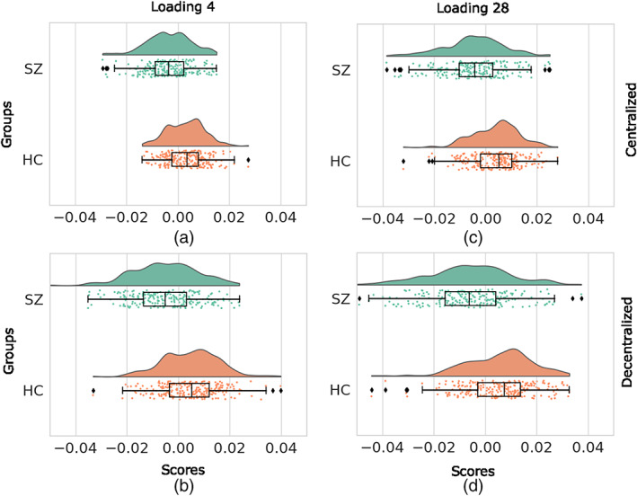
Cloud plot of adjusted loading parameters 4 and 28. Panels (a) and (b) represent the cloud plot of adjusted loading parameters 4 for the centralized and decentralized analysis, respectively. Panels (c) and (d) represent the plot of adjusted loading parameters 28 for the centralized and decentralized analysis, respectively. In each panel, upper plot (Green) and lower (Brown) plots are the clouds of loading score for the patients and healthy controls, respectively.

From our regression model, we computed the effect size for the independent variables age, gender, and diagnosis for both centralized and decentralized analyses. We present our results in Figure 4. In the figure, panels (a), (b), and (c) are the scatter plots of the centralized versus decentralized effect sizes for the variables age, gender, and diagnosis, respectively. In each panel, we observe that the points largely follow the identity line. These plots demonstrate that the obtained centralized and decentralized effect sizes are very similar. Based on the effect sizes of diagnosis for the centralized case being ${\epsilon }^2>0.02$, we identified seven independent sources. The spatial maps of these sources are presented in Figure 5. Notice that although the effect sizes in the decentralized case tend to be slightly inflated with respect to the centralized case, only a couple of false positives occur for diagnosis (our effect of interest). We also computed the p value for the variables age, gender, and diagnosis obtained from our linear regression model and finally compared the decentralized results with the P values from the centralized analysis. We present the experimental results in Figure 6. In the figure, panels (a), (b), and (c) demonstrate the scatter plots of centralized versus decentralized p values for the variables age, gender, and diagnosis, respectively. Here, we find very similar p values for centralized and decentralized analyses, in close correspondence with the patterns observed for effect sizes.

FIGURE 4.

Scatter plot between the centralized and decentralized effect sizes. Panels (a), (b), and (c) correspond to variables age, gender, and diagnosis, respectively. Scatter plots of centralized and decentralized effect sizes exhibit high consistency.

FIGURE 5.

Visual summary of sources with large effect sizes.

FIGURE 6.

Scatter plot of centralized versus decentralized p values. The values are presented in log–log scale. Panels (a), (b), and (c) correspond to variables age, gender, and diagnosis, respectively. The similar p values for centralized and decentralized analysis indicate high consistency.

To examine the reliability of our dcSBM approach, we utilized the UK Biobank data set. We present the experimental results in Figure 7 (Section 2.5.3: random shuffle). Figure 7a represents the similarity between the centralized and decentralized loading parameters. The performance measures correlation, MSE, MaxAE, and MedianAE are among the correlation matrices shown in Figure 2a,b obtained for the UKBiobank data set, for each of the 10 shuffled runs. Each MSE, MaxAE, and MedianAE are normalized by the mean‐squared, max‐abs, and median‐abs of centralized correlations matrices, respectively. Figure 7b represents the similarity between the centralized source correlation matrix and the centralized versus decentralized source correlation matrix. In the figure, each boxplot consists of 10 points from different 10 shuffled runs, and we find that all points are very similar, which eventually implies high reliability. Figure 8 represents the results of Section 2.5.3: increasing number of sites, each with the same number of subjects. After running the experiment for each site, we collect the correlation matrices (as in Figure 2a,b and report the correlation and MSE between them. We also compute these metrics for the source correlation matrices. Results are presented in Figure 8a,b, respectively. In both plots, we observe very high correlation between the centralized and decentralized results, with the correlations decreasing and MSE increasing slightly as the total number of sites participating in the analysis increases. Figure 9 represents the results of Section 2.5.3: Increase number of samples in global consortia. To assess the correlation and mean squared error (MSE) between the correlation matrices of six sites and all other sites (sites 2–6), we present the results in Figure 9a. Here, we observe that as the number of samples increases in the centralized setup, the correlation also increases, and the MSE decreases. In Figure 9b, we presented the correlation and MSE between the correlation metrics obtained from the pooled subjects and each decentralized experiment. We observed an increased correlation and a decrease in MSE as the number of sites (and consequently the number of samples in the global consortia) increased.

FIGURE 7.

Similarity metrics of loading parameters and sources. Panels (a) and (b) represent the similarity metrics of loading parameters and sources, respectively. The left Y‐axis represents the correlation measure and the right Y‐axis represents mean square error, max absolute error, and median absolute error.

FIGURE 8.

Similarity metrics for loading parameters and sources. Panels (a) and (b) represent the similarity metrics of loading parameters and sources, respectively, for increasing number of sites. The left Y‐axis and right Y‐axis are utilized for correlation and mean square error (MSE), respectively.

FIGURE 9.

Similarity metrics for loading parameters. Panels (a) and (b) represent the similarity metrics of loading parameters in centralized and decentralized setups. The left Y‐axis and right Y‐axis are utilized for correlation and mean square error (MSE), respectively.

4. DISCUSSION

The use of structural MRI data to study brain morphometry continues to grow. SMRI features have been successfully applied to examine structure and function alterations in different domains (Hirjak et al., 2022; Wolf et al., 2020), patient classifications (Abrol et al., 2021; Arbabshirani et al., 2013; Yao et al., 2018), and have also been combined in various multimodal studies (Abrol et al., 2019; Sui et al., 2014). However, in scenarios where data is only locally accessible and cannot be pooled in a central location, existing established algorithms, including constrained SBM, cannot operate. To overcome this limitation, we have introduced the use of a fully automated brain‐wide decentralized constrained SBM algorithm to operate within decentralized environments.

In our analysis, we extracted 30 independent components from both centralized and decentralized cSBM. To analyze the pairwise correlation, we computed the correlation among each column of the centralized and decentralized loading parameters. For comparative analysis, we also evaluated the correlations among the centralized and decentralized source matrices. The results are presented in Figure 2. From our statistical analysis, we observed that the centralized and decentralized result estimates are very similar. That is why the diagonal exhibits the highest correlations in the correlation metric. We also observed that if the centralized estimates extract any structural patterns, these patterns are also reflected in our decentralized results.

Recently, many studies have been conducted to analyze the effects of age, gender, and diagnosis (Gupta et al., 2015; Haijma et al., 2013; Hoffman et al., 2022; Holleran et al., 2020; Segall et al., 2012; Turner et al., 2012; Turner et al., 2013; Van Erp et al., 2014) on gray matter. In our regression analysis, we consider age, gender, diagnosis, site, and the possible interactions between them as the predictors. The loading parameters recovered from local constrained ICAs are considered as the dependent variables. We computed the $p$ value for the variables age, gender, and diagnosis for both centralized and decentralized SBM. The results are presented in Figure 6. We computed the minimum, maximum, and standard deviation from the obtained $p$ values. We summarize the centralized versus decentralized $p$ values in Table 1. In the table, c‐min, d‐min, c‐max, d‐max, c‐std, and d‐std represent the centralized minimum, decentralized minimum, centralized maximum, decentralized maximum, centralized standard deviation, and decentralized standard deviation, respectively. The results mostly align across the diagonal. We also computed the effect size of variables age, gender, and diagnosis on loading parameters. The results are presented in Table 2. Here, the results from both cSBM and our dcSBM exhibit similar patterns, aligning across the diagonal in the plots. All in all, these experimental results establish the hypothesis that our dcSBM produces very close results compared to cSBM.

TABLE 1.

Centralized versus decentralized p values.

Variables	c‐min	d‐min	c‐max	d‐max	c‐std	d‐std
Age	.0000	.0000	.9846	.9685	.3084	.2908
Gender	.0000	.0000	.9505	.8132	.2790	.2426
Diagnosis	.0000	.0000	.8507	.9377	.2997	.3329

Abbreviations: c‐max, centralized maximum; c‐min, centralized minimum; c‐std, centralized standard deviation; d‐max, decentralized maximum; d‐min, decentralized minimum; d‐std, decentralized standard deviation.

TABLE 2.

Centralized versus decentralized effect sizes.

Variables	c‐min	d‐min	c‐max	d‐max	c‐std	d‐std
Age	−0.0023	−0.0023	0.0616	0.0761	0.0168	0.0223
Gender	−0.0023	−0.0022	0.2562	0.2567	0.0471	0.0483
Diagnosis	−0.0022	−0.0023	0.0760	0.0950	0.0191	0.0225

Abbreviations: c‐max, centralized maximum; c‐min, centralized minimum; c‐std, centralized standard deviation; d‐max, decentralized maximum; d‐min, decentralized minimum; d‐std, decentralized standard deviation.

We conducted these experiments on real data from seven sites for fBIRN and a single site for COBRE. The references used in the patient data set were organized into eight different domains: five components in the visual (VS) domain, nine in the cerebellum (CB) domain, three in the frontal (FN) domain, two in the default‐mode (DMN) domain, two in the subcortical (SC) domain, two in the sensorimotor (SM) domain, two in the insula (IS) domain, and one in the hippocampus (HIP) domain. The spatial maps of these eight different brain regions from our analysis are presented in Figure 10. In our regression analysis, we considered the site effects, including their interaction with age, gender, and diagnosis. However, we did not find any significant effects from site on the response variables. Based on the effect sizes from diagnosis, we identified seven components (out of 30 components) with significant effect sizes. Among those eight components, component 4 covers the insula, temporal pole, frontal orbital cortex, anterior cingulate, and parahippocampal domains; component 28 covers the regions of the anterior and dorsolateral prefrontal cortex; component 14 covers insula and parietal areas; component 17 covers cerebellum and subcortical areas; component 24 covers additional regions of the cerebellum; component 16 covers putamen and caudate nucleus (subcortical), and component 18 covers vermis and declive of the cerebellum. Several studies have investigated the effect size of diagnosis and reported their results. Based on the effect size, Navin et al. reported the largest difference in gray matter concentration between diagnostic groups, including regions in the insula, superior temporal gyrus, superior frontal gyrus, temporal gyrus, hippocampus, cerebellum, and some other regions (Gupta et al., 2015). Tomas et al. also reported reductions in gray matter in prefrontal, temporal, and cerebellar regions among first‐episode SZ patients (Kašpárek et al., 2010). These effect size findings provide additional support for the validity of our own findings.

FIGURE 10.

Visual summary of components in eight different brain regions: five components in visual (VS), nine in cerebellum (CB), three in frontal (FN), two in default‐mode (DMN), two in subcortical (SC), two in sensorimotor (SM), two in insula (IS), and one in hippocampus (HIP) domain.

Finally, we deployed our approach within an open‐source federated neuroimaging analysis tool called COINSTAC.3 This provides a user‐friendly way for users to build consortia and utilize the proposed dcSBM approach. COINSTAC also allows the creation of persistent nodes, called vaults. The data in this paper will be released via a COINSTAC vault, providing a perfect example use case, as some of the data are not openly shareable due to IRB restrictions but can be analyzed via the federated approach (Martin et al., 2023).

We acknowledge that the estimated loading parameters produced with dcSBM have larger values than the centralized counterparts. This is possibly due to the known scaling ambiguity in ICA. While this could pose issues such as inflation of site effects in our proposed decentralized setting, our statistical analysis modeled such effects in a way that mitigates these concerns (i.e., using linear interaction terms with site). Additionally, we did not explicitly address the issue of non‐IIDness in our analysis. If the sites involved are not independent and identically distributed, it is possible for the local estimates to deviate from the ideal centralized outcomes. In our current study, we did not specifically account for this issue because it remains an open problem even in the centralized case. As a result, we conducted our analysis under the assumption of an identical distribution across all sites. However, we recognize that work on data harmonization (Bostami et al., 2021) to address non‐IIDness is valuable, and exploring decentralized extensions of these approaches is important for further improvement in our approach. We plan to experiment with this in future work to enhance the robustness of our method.

4.1. Decentralized regression without exposing the loading parameters

In our approach, a master node accumulates the mixing and source matrices from each site to perform statistical analysis at a central site. We understand that this aggregate statistical operation may raise privacy concerns. However, it is essential to note that our primary objective was to demonstrate that the decentralized constrained SBM can closely replicate the centralized estimates. In our analysis, we concatenated loading parameters from each site in an aggregator and conducted regression analysis centrally. Nevertheless, it is also possible to conduct the linear regression analysis in a fully distributed manner. For decentralized regression, we refer the reader to (Gazula et al., 2018). In summary, we can write the least squares solution for the regression parameter $\widehat{\beta }$ as:

$$\widehat{\beta }=\left(\sum _{\mathrm{\ell }=1}^L{Z}_{\mathrm{\ell }}^{{\rm T}}{Z}_{\mathrm{\ell }}\right)\left(\sum _{\mathrm{\ell }=1}^L{Z}_{\mathrm{\ell }}^{{\rm T}}{a}_{\mathrm{\ell }}\right)$$ (1)

In Equation (1), $a_{\mathrm{\ell }}$ is the response variable we would like to predict, here the loading parameters learned locally in site $\mathrm{\ell }$ based on the linear model $a\approx \mathit{Z\beta }$, where $Z$ is the matrix containing predictors in each column, and $\beta$ is the regression parameter. In a decentralized environment with $L$ sites, $Z$ can be represented by $Z={\left[Z_1^T,Z_2^T,\dots ,Z_L^T\right]}^T$, and $a$ can be defined by $a={\left[a_1^T,a_2^T,\dots ,a_L^T\right]}^T$. In this approach, $a_{\mathrm{\ell }}$ and $Z_{\mathrm{\ell }}$ do not have to be transmitted/aggregated, improving the privacy. Only the terms $Z_{\mathrm{\ell }}^{{\rm T}}{Z}_{\mathrm{\ell }}$ and $Z_{\mathrm{\ell }}^{{\rm T}}{a}_{\mathrm{\ell }}$ are transmitted/aggregated. This approach is capable of generating identical results as our simple aggregator and has been integrated to COINSTAC4 (Gazula et al., 2020; Plis et al., 2016). Finally, it is worth mentioning that in our approach, the source matrices were aggregated from each site only for the purpose of quality control assessment of our proposed approach. It is recommended that each site retain its source estimates ($S_{\mathrm{\ell }}$) to minimize risks of privacy leaks (note that, by definition, the local data $X_{\mathrm{\ell }}$ can be reconstructed from $A_{\mathrm{\ell }}$ and $S_{\mathrm{\ell }}$).

5. CONCLUSION

In this work, we first propose a fully automated cSBM approach and then develop an approach to utilize constrained SBM in a decentralized manner. We utilized two different real multisite data sets for our statistical analysis. In our experiment, we considered age, gender, diagnosis, and site effects and evaluated the similarity between centralized and decentralized constrained SBM. We also investigated the reliability of our algorithm using the UKBiobank data set. In all experiments, our decentralized approach generates very close results that very closely replicate the centralized estimates. In all experiments, our decentralized approach generates very close results that very closely replicate the centralized estimates. Group difference testing identified two significant sources, one covering the insula, temporal pole, frontal orbital cortex, anterior cingulate, and parahippocampal domains, and another covering the anterior and dorsolateral prefrontal cortices. We also deployed our dcSBM approach in the COINSTAC application to provide a user‐friendly platform for individuals to establish consortia and make use of the benefits of our proposed dcSBM approach. For future work, we will implement a decentralized regression approach to conduct our experiment without results aggregation. Finally, our algorithm allows for the analysis of private local site data that cannot be shared while still leveraging its utility via decentralized computation.

CONFLICT OF INTEREST STATEMENT

The authors declare no conflicts of interest.

Saha, D. K. , Silva, R. F. , Baker, B. T. , Saha, R. , & Calhoun, V. D. (2023). dcSBM: A federated constrained source‐based morphometry approach for multivariate brain structure mapping. Human Brain Mapping, 44(17), 5892–5905. 10.1002/hbm.26483

DATA AVAILABILITY STATEMENT

The data that support the findings of this study are available on request from the corresponding author. The data are not publicly available due to privacy or ethical restrictions. The experimental code will be available upon request from the corresponding author.

REFERENCES

- Abrol, A. , Fu, Z. , Du, Y. , & Calhoun, V. D. (2019). Multimodal data fusion of deep learning and dynamic functional connectivity features to predict Alzheimer's disease progression. In 2019 41st annual international conference of the IEEE engineering in medicine and biology society (EMBC) (pp. 4409–4413). IEEE. [DOI] [PubMed] [Google Scholar]
- Abrol, A. , Fu, Z. , Salman, M. , Silva, R. , Du, Y. , Plis, S. , & Calhoun, V. (2021). Deep learning encodes robust discriminative neuroimaging representations to outperform standard machine learning. Nature Communications, 12(1), 1–17. [DOI] [PMC free article] [PubMed] [Google Scholar]
- Aine, C. , Bockholt, H. J. , Bustillo, J. R. , Cañive, J. M. , Caprihan, A. , Gasparovic, C. , Hanlon, F. M. , Houck, J. M. , Jung, R. E. , Lauriello, J. , Liu, J. , Mayer, A. R. , Perrone‐Bizzozero, N. I. , Posse, S. , Stephen, J. M. , Turner, J. A. , Clark, V. P. , & Calhoun, V. D. (2017). Multimodal neuroimaging in schizophrenia: Description and dissemination. Neuroinformatics, 15(4), 343–364. [DOI] [PMC free article] [PubMed] [Google Scholar]
- Arbabshirani, M. R. , Kiehl, K. A. , Pearlson, G. D. , & Calhoun, V. D. (2013). Classification of schizophrenia patients based on resting‐state functional network connectivity. Frontiers in Neuroscience, 7, 133. [DOI] [PMC free article] [PubMed] [Google Scholar]
- Bostami, B. , Calhoun, V. D. , Van Der Horn, H. J. , & Vergara, V. (2021). Harmonization of multi‐site dynamic functional connectivity network data. In 2021 IEEE 21st international conference on bioinformatics and bioengineering (BIBE) (pp. 1–4). IEEE. [Google Scholar]
- Calhoun, V. D. , Liu, J. , & Adal, T. (2009). A review of group ICA for fMRI data and ICA for joint inference of imaging, genetic, and ERP data. NeuroImage, 45(1), S163–S172. [DOI] [PMC free article] [PubMed] [Google Scholar]
- Du, Y. , & Fan, Y. (2013). Group information guided ICA for fMRI data analysis. NeuroImage, 69, 157–197. [DOI] [PubMed] [Google Scholar]
- Du, Y. , Fu, Z. , Sui, J. , Gao, S. , Xing, Y. , Lin, D. , Salman, M. , Abrol, A. , Rahaman, M. A. , Chen, J. , Hong, L. E. , Kochunov, P. , Osuch, E. A. , Calhoun, V. D. , & Alzheimer's Disease Neuroimaging Initiative . (2020). NeuroMark: An automated and adaptive ICA based pipeline to identify reproducible fMRI markers of brain disorders. NeuroImage: Clinical, 28, 102375. [DOI] [PMC free article] [PubMed] [Google Scholar]
- Gazula, H. , Baker, B. T. , Damaraju, E. , Plis, S. M. , Panta, S. R. , Silva, R. F. , & Calhoun, V. D. (2018). Decentralized analysis of brain imaging data: Voxel‐based morphometry and dynamic functional network connectivity. Frontiers in Neuroinformatics, 12, 55. [DOI] [PMC free article] [PubMed] [Google Scholar]
- Gazula, H. , Holla, B. , Zhang, Z. , Xu, J. , Verner, E. , Kelly, R. , Jain, S. , Bharath, R. D. , Barker, G. J. , Basu, D. , Chakrabarti, A. , Kalyanram, K. , Kumaran, K. , Singh, L. , Kuriyan, R. , Murthy, P. , Benega, V. , Plis, S. M. , Sarwate, A. D. , … Calhoun, V. D. (2021). Decentralized multisite VBM analysis during adolescence shows structural changes linked to age, body mass index, and smoking: A COINSTAC analysis. Neuroinformatics, 19(4), 553–566. [DOI] [PMC free article] [PubMed] [Google Scholar]
- Gazula, H. , Kelly, R. , Romero, J. , Verner, E. , Baker, B. T. , Silva, R. F. , Imtiaz, H. , Saha, D. , Raja, R. , Turner, J. , Sarwate, A. , Plis, S. , & Calhoun, V. (2020). Coinstac: Collaborative informatics and neuroimaging suite toolkit for anonymous computation. Journal of Open Source Software, 5(54), 2166. [Google Scholar]
- Good, C. D. , Johnsrude, I. S. , Ashburner, J. , Henson, R. N. , Friston, K. J. , & Frackowiak, R. S. (2001). A voxel‐based morphometric study of ageing in 465 normal adult human brains. NeuroImage, 14(1), 21–36. [DOI] [PubMed] [Google Scholar]
- Grecucci, A. , Rubicondo, D. , Siugzdaite, R. , Surian, L. , & Job, R. (2016). Uncovering the social deficits in the autistic brain. A source‐based morphometric study. Frontiers in Neuroscience, 10, 388. [DOI] [PMC free article] [PubMed] [Google Scholar]
- Gupta, C. N. , Calhoun, V. D. , Rachakonda, S. , Chen, J. , Patel, V. , Liu, J. , Segall, J. , Franke, B. , Zwiers, M. P. , Arias‐Vasquez, A. , Buitelaar, J. , Fisher, S. E. , Fernandez, G. , van Erp, T. G. M. , Potkin, S. , Ford, J. , Mathalon, D. , McEwen, S. , Lee, H. J. , … Turner, J. A. (2015). Patterns of gray matter abnormalities in schizophrenia based on an international mega‐analysis. Schizophrenia Bulletin, 41(5), 1133–1142. [DOI] [PMC free article] [PubMed] [Google Scholar]
- Gupta, C. N. , Turner, J. A. , & Calhoun, V. D. (2019). Source‐based morphometry: A decade of covarying structural brain patterns. Brain Structure and Function, 224(9), 3031–3044. [DOI] [PubMed] [Google Scholar]
- Haijma, S. V. , Van Haren, N. , Cahn, W. , Koolschijn, P. C. M. , Hulshoff Pol, H. E. , & Kahn, R. S. (2013). Brain volumes in schizophrenia: A meta‐analysis in over 18 000 subjects. Schizophrenia Bulletin, 39(5), 1129–1138. [DOI] [PMC free article] [PubMed] [Google Scholar]
- Hirjak, D. , Schmitgen, M. M. , Werler, F. , Wittemann, M. , Kubera, K. M. , Wolf, N. D. , Sambataro, F. , Calhoun, V. D. , Reith, W. , & Wolf, R. C. (2022). Multimodal MRI data fusion reveals distinct structural, functional and neurochemical correlates of heavy cannabis use. Addiction Biology, 27(2), e13113. [DOI] [PubMed] [Google Scholar]
- Hoffman, G. E. , Ma, Y. , Montgomery, K. S. , Bendl, J. , Jaiswal, M. K. , Kozlenkov, A. , Peters, M. A. , Dracheva, S. , Fullard, J. F. , Chess, A. , Devlin, B. , Sieberts, S. K. , & Roussos, P. (2022). Sex differences in the human brain transcriptome of cases with schizophrenia. Biological Psychiatry, 91(1), 92–101. [DOI] [PMC free article] [PubMed] [Google Scholar]
- Holleran, L. , Kelly, S. , Alloza, C. , Agartz, I. , Andreassen, O. A. , Arango, C. , Banaj, N. , Calhoun, V. , Cannon, D. , Carr, V. , Corvin, A. , Glahn, D. C. , Gur, R. , Hong, E. , Hoschl, C. , Howells, F. M. , James, A. , Janssen, J. , Kochunov, P. , … Donohoe, G. (2020). The relationship between white matter microstructure and general cognitive ability in patients with schizophrenia and healthy participants in the ENIGMA consortium. American Journal of Psychiatry, 177(6), 537–547. [DOI] [PMC free article] [PubMed] [Google Scholar]
- Kašpárek, T. , Mareček, R. , Schwarz, D. , Přikryl, R. , Vanček, J. , Mikl, M. , & Cesková, E. (2010). Source‐based morphometry of gray matter volume in men with first‐episode schizophrenia. Human Brain Mapping, 31(2), 300–310. [DOI] [PMC free article] [PubMed] [Google Scholar]
- Lapomarda, G. , Grecucci, A. , Messina, I. , Pappaianni, E. , & Dadomo, H. (2021). Common and different gray and white matter alterations in bipolar and borderline personality disorder: A source‐based morphometry study. Brain Research, 1762, 147401. [DOI] [PubMed] [Google Scholar]
- Lin, Q. H. , Liu, J. , Zheng, Y. R. , Liang, H. , & Calhoun, V. D. (2010). Semiblind spatial ICA of fMRI using spatial constraints. Human Brain Mapping, 31(7), 1076–1088. [DOI] [PMC free article] [PubMed] [Google Scholar]
- Lu, W. , & Rajapakse, J. C. (2005). Approach and applications of constrained ICA. IEEE Transactions on Neural Networks, 16(1), 203–212. [DOI] [PubMed] [Google Scholar]
- Luo, L. , Xu, L. , Jung, R. , Pearlson, G. , Adali, T. , & Calhoun, V. D. (2012). Constrained source‐based morphometry identifies structural networks associated with default mode network. Brain Connectivity, 2(1), 33–43. [DOI] [PMC free article] [PubMed] [Google Scholar]
- Martin, D. , Basodi, S. , Panta, S. , Rootes‐Murdy, K. , Prae, P. , Sarwate, A. D. , Kelly, R. , Romero, J. , Baker, B. T. , Gazula, H. , Bockholt, J. , Turner, J. A. , Esper, N. B. , Franco, A. R. , Plis, S. , & Calhoun, V. D. (2023). Enhancing collaborative neuroimaging research: Introducing COINSTAC vaults for federated analysis and reproducibility. Frontiers in Neuroinformatics, 17, 1207721. [DOI] [PMC free article] [PubMed] [Google Scholar]
- Mennes, M. , Jenkinson, M. , Valabregue, R. , Buitelaar, J. K. , Beckmann, C. , & Smith, S. (2014). Optimizing full‐brain coverage in human brain MRI through population distributions of brain size. NeuroImage, 98, 513–520. [DOI] [PubMed] [Google Scholar]
- Pappaianni, E. , Siugzdaite, R. , Vettori, S. , Venuti, P. , Job, R. , & Grecucci, A. (2018). Three shades of grey: Detecting brain abnormalities in children with autism using source‐, voxel‐and surface‐based morphometry. European Journal of Neuroscience, 47(6), 690–700. [DOI] [PubMed] [Google Scholar]
- Pearlson, G. D. , Liu, J. , & Calhoun, V. D. (2015). An introductory review of parallel independent component analysis (p‐ICA) and a guide to applying p‐ICA to genetic data and imaging phenotypes to identify disease‐associated biological pathways and systems in common complex disorders. Frontiers in Genetics, 6, 276. [DOI] [PMC free article] [PubMed] [Google Scholar]
- Plis, S. M. , Sarwate, A. D. , Wood, D. , Dieringer, C. , Landis, D. , Reed, C. , Panta, S. R. , Turner, J. A. , Shoemaker, J. M. , Carter, K. W. , Thompson, P. , Hutchison, K. , & Calhoun, V. D. (2016). COINSTAC: A privacy enabled model and prototype for leveraging and processing decentralized brain imaging data. Frontiers in Neuroscience, 10, 365. [DOI] [PMC free article] [PubMed] [Google Scholar]
- Premi, E. , Calhoun, V. , Garibotto, V. , Turrone, R. , Alberici, A. , Cottini, E. , Pilotto, A. , Gazzina, S. , Magoni, M. , Paghera, B. , Borroni, B. , & Padovani, A. (2017). Source‐based morphometry multivariate approach to analyze [123I] FP‐CIT SPECT imaging. Molecular Imaging and Biology, 19(5), 772–778. [DOI] [PMC free article] [PubMed] [Google Scholar]
- Rahaman, M. A. , Damaraju, E. , Saha, D. K. , Plis, S. M. , & Calhoun, V. D. (2022). Statelets: Capturing recurrent transient variations in dynamic functional network connectivity. Human Brain Mapping, 43(8), 2503–2518. 10.1002/hbm.25799 [DOI] [PMC free article] [PubMed] [Google Scholar]
- Rissman, J. , & Wagner, A. D. (2012). Distributed representations in memory: Insights from functional brain imaging. Annual Review of Psychology, 63, 101–128. [DOI] [PMC free article] [PubMed] [Google Scholar]
- Saha, D. K. , Calhoun, V. D. , Du, Y. , Fu, Z. , Kwon, S. M. , Sarwate, A. D. , Panta, S. R. , & Plis, S. M. (2022). Privacy‐preserving quality control of neuroimaging datasets in federated environments. Human Brain Mapping, 43(7), 2289–2310. [DOI] [PMC free article] [PubMed] [Google Scholar]
- Saha, D. K. , Calhoun, V. D. , Panta, S. R. , & Plis, S. M. (2017). See without looking: Joint visualization of sensitive multi‐site datasets (pp. 2672–2678). IJCAI. [Google Scholar]
- Saha, D. K. , Damaraju, E. , Rashid, B. , Abrol, A. , Plis, S. M. , & Calhoun, V. D. (2021). A classification‐based approach to estimate the number of resting functional magnetic resonance imaging dynamic functional connectivity states. Brain Connectivity, 11(2), 132–145. 10.1089/brain.2020.0794 [DOI] [PMC free article] [PubMed] [Google Scholar]
- Saha, D. K. , Silva, R. F. , Baker, B. T. , & Calhoun, V. D. (2022). Decentralized spatially constrained source‐based morphometry. In 2022 IEEE 19th international symposium on biomedical imaging (ISBI) (pp. 1–5). IEEE. [Google Scholar]
- Saha, R. , Saha, D. K. , Abdur Rahaman, M. , Fu, Z. , Calhoun, V. D. (2022). Longitudinal whole‐brain functional network change patterns over a two‐year period in the ABCD Data. In 2022 IEEE 19th international symposium on biomedical imaging (ISBI) (pp. 1–4).
- Segall, J. M. , Allen, E. A. , Jung, R. E. , Erhardt, E. B. , Arja, S. K. , Kiehl, K. , & Calhoun, V. D. (2012). Correspondence between structure and function in the human brain at rest. Frontiers in Neuroinformatics, 6, 10. [DOI] [PMC free article] [PubMed] [Google Scholar]
- Sorella, S. , Lapomarda, G. , Messina, I. , Frederickson, J. J. , Siugzdaite, R. , Job, R. , & Grecucci, A. (2019). Testing the expanded continuum hypothesis of schizophrenia and bipolar disorder. Neural and psychological evidence for shared and distinct mechanisms. NeuroImage: Clinical, 23, 101854. [DOI] [PMC free article] [PubMed] [Google Scholar]
- Sui, J. , Adali, T. , Yu, Q. , Chen, J. , & Calhoun, V. D. (2012). A review of multivariate methods for multimodal fusion of brain imaging data. Journal of Neuroscience Methods, 204(1), 68–81. [DOI] [PMC free article] [PubMed] [Google Scholar]
- Sui, J. , Huster, R. , Yu, Q. , Segall, J. M. , & Calhoun, V. D. (2014). Function–structure associations of the brain: Evidence from multimodal connectivity and covariance studies. NeuroImage, 102, 11–23. [DOI] [PMC free article] [PubMed] [Google Scholar]
- Sweeney, L. (2002). k‐anonymity: A model for protecting privacy. International Journal of Uncertainty, Fuzziness and Knowledge‐Based Systems, 10(5), 557–570. [Google Scholar]
- Sweeney, L. , Crosas, M. , & Bar‐Sinai, M. (2015). Sharing sensitive data with confidence: The datatags system. Technology. Science, 2015101601. https://techscience.org/a/2015101601/ [Google Scholar]
- Turner, J. A. , Calhoun, V. D. , Michael, A. , Van Erp, T. G. , Ehrlich, S. , Segall, J. M. , Gollub, R. L. , Csernansky, J. , Potkin, S. G. , Ho, B. C. , Bustillo, J. , Schulz, S. C. , FBIRN , & Wang, L. (2012). Heritability of multivariate gray matter measures in schizophrenia. Twin Research and Human Genetics, 15(3), 324–335. [DOI] [PMC free article] [PubMed] [Google Scholar]
- Turner, J. A. , Damaraju, E. , Van Erp, T. G. , Mathalon, D. H. , Ford, J. M. , Voyvodic, J. , Mueller, B. A. , Belger, A. , Bustillo, J. , McEwen, S. , Potkin, S. G. , FBIRN , & Calhoun, V. D. (2013). A multi‐site resting state fMRI study on the amplitude of low frequency fluctuations in schizophrenia. Frontiers in Neuroscience, 7, 137. [DOI] [PMC free article] [PubMed] [Google Scholar]
- Van Erp, T. G. , Greve, D. N. , Rasmussen, J. , Turner, J. , Calhoun, V. D. , Young, S. , Mueller, B. , Brown, G. G. , McCarthy, G. , Glover, G. H. , Lim, K. O. , Bustillo, J. R. , Belger, A. , McEwen, S. , Voyvodic, J. , Mathalon, D. H. , Keator, D. , Preda, A. , Nguyen, D. , … FBIRN . (2014). A multi‐scanner study of subcortical brain volume abnormalities in schizophrenia. Psychiatry Research: Neuroimaging, 222(1–2), 10–16. [DOI] [PMC free article] [PubMed] [Google Scholar]
- Wolf, R. C. , Rashidi, M. , Fritze, S. , Kubera, K. M. , Northoff, G. , Sambataro, F. , Calhoun, V. D. , Geiger, L. S. , Tost, H. , & Hirjak, D. (2020). A neural signature of parkinsonism in patients with schizophrenia spectrum disorders: A multimodal MRI study using parallel ICA. Schizophrenia Bulletin, 46(4), 999–1008. [DOI] [PMC free article] [PubMed] [Google Scholar]
- Xu, L. , Groth, K. M. , Pearlson, G. , Schretlen, D. J. , & Calhoun, V. D. (2009). Source‐based morphometry: The use of independent component analysis to identify gray matter differences with application to schizophrenia. Human Brain Mapping, 30(3), 711–724. [DOI] [PMC free article] [PubMed] [Google Scholar]
- Yao, D. , Calhoun, V. D. , Fu, Z. , Du, Y. , & Sui, J. (2018). An ensemble learning system for a 4‐way classification of Alzheimer's disease and mild cognitive impairment. Journal of Neuroscience Methods, 302, 75–81. [DOI] [PMC free article] [PubMed] [Google Scholar]
Associated Data
This section collects any data citations, data availability statements, or supplementary materials included in this article.