Spreadsheet Method for Evaluation of Biochemical Reaction Rate Coefficients and Their Uncertainties by Weighted Nonlinear Least-Squares Analysis of the Integrated Monod Equation

Abstract

A convenient method for evaluation of biochemical reaction rate coefficients and their uncertainties is described. The motivation for developing this method was the complexity of existing statistical methods for analysis of biochemical rate equations, as well as the shortcomings of linear approaches, such as Lineweaver-Burk plots. The nonlinear least-squares method provides accurate estimates of the rate coefficients and their uncertainties from experimental data. Linearized methods that involve inversion of data are unreliable since several important assumptions of linear regression are violated. Furthermore, when linearized methods are used, there is no basis for calculation of the uncertainties in the rate coefficients. Uncertainty estimates are crucial to studies involving comparisons of rates for different organisms or environmental conditions. The spreadsheet method uses weighted least-squares analysis to determine the best-fit values of the rate coefficients for the integrated Monod equation. Although the integrated Monod equation is an implicit expression of substrate concentration, weighted least-squares analysis can be employed to calculate approximate differences in substrate concentration between model predictions and data. An iterative search routine in a spreadsheet program is utilized to search for the best-fit values of the coefficients by minimizing the sum of squared weighted errors. The uncertainties in the best-fit values of the rate coefficients are calculated by an approximate method that can also be implemented in a spreadsheet. The uncertainty method can be used to calculate single-parameter (coefficient) confidence intervals, degrees of correlation between parameters, and joint confidence regions for two or more parameters. Example sets of calculations are presented for acetate utilization by a methanogenic mixed culture and trichloroethylene cometabolism by a methane-oxidizing mixed culture. An additional advantage of application of this method to the integrated Monod equation compared with application of linearized methods is the economy of obtaining rate coefficients from a single batch experiment or a few batch experiments rather than having to obtain large numbers of initial rate measurements. However, when initial rate measurements are used, this method can still be used with greater reliability than linearized approaches.

The evaluation of bacterial and enzymatic reaction rates requires representative rate data and a valid method for fitting appropriate rate equations to the data. In addition, estimation of uncertainties in rate coefficients is crucial for informed comparisons between cultures or environmental conditions. Nonlinear least-squares analysis of nonlinear equations, such as the Monod and Michaelis-Menten equations, can provide accurate estimates of rate coefficients and reliable estimates of the uncertainties in the coefficients.

Transformations of the nonlinear rate equations to linear forms, such as Lineweaver-Burk and Eadie-Hofstee plots, are undesirable for numerous reasons that have been discussed repeatedly (3, 5, 9, 10). The deficiencies in the use of linearized forms have been recognized for many years (6) but have often been overlooked due to the time-consuming calculations and complexity of nonlinear least-squares analysis.

The integrated Monod equation is useful in many applications for evaluation of bacterial transformation rate coefficients. Coefficients can be evaluated from progress curves from a few batch experiments or even one batch experiment of a reaction. This fact can be very important when data are costly to obtain, such as in animal studies or human studies.

However, the integrated Monod equation is somewhat cumbersome to use because it is a nonlinear implicit expression for substrate and organism concentrations. Weighted least-squares analysis is an approach that can be used to minimize differences between experimental data and model predictions when it is necessary to use an implicit expression in the model. This paper describes a simple method for determining the best-fit values for rate coefficients in the Monod equation and their uncertainties by using weighted least-squares analysis. The method is straightforward and is designed for easy implementation in a computer spreadsheet program. As examples, results from two rate studies were used together with an integrated Monod equation weighted least-squares analysis to determine rate coefficients and their uncertainties. A simple example involving a data set for acetate utilization by a methanogenic mixed culture is described. A second, more complex data set for trichloroethylene (TCE) cometabolism by a methane-oxidizing mixed culture is used to illustrate application of this method to cometabolism and verification of the method by comparison with a more rigorous numerical model. The experimental techniques used are described elsewhere (7, 12).

MATERIALS AND METHODS

Integrated Monod equation.

An integrated form of the Monod equation for utilization or cometabolism of a substrate in a batch reactor can be obtained. The Monod equation for the substrate reaction rate in a bacterial culture is

1

where C_L is the liquid-phase concentration of the rate-limiting substrate (in milligrams per liter), t is time (in days), k is the maximum specific rate of substrate utilization (in milligrams of substrate per milligram of active cells per day), X_a is the concentration of active cells (in milligrams per liter), and K_S is the half-velocity coefficient (in milligrams of substrate per liter).

The active cell concentration with growth substrate utilization can be described by

2

where Y is the cell yield coefficient (in grams of active cells per gram of substrate) and the subscript 0 denotes time zero.

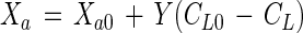
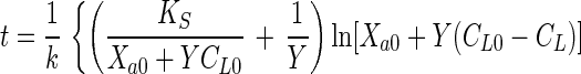
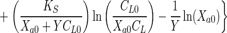
Equations 1 and 2 can be combined to eliminate X_a and can be integrated to obtain the integrated Monod equation for a growth substrate

3

Alternatively, when a volatile nongrowth substrate, such as TCE, is cometabolized in the absence of growth substrate, it is necessary to account for the gas-liquid partitioning of the substrate and the effect of TCE transformation product toxicity. For gaseous substrates, a mass balance on a closed system gives

4

where M is the mass of substrate present (in milligrams), C_G is the gas-phase substrate concentration (in milligrams per liter), V_L is the liquid volume (in liters), and V_G is the gas volume (in liters).

Henry’s Law (11) can be used to account for the distribution of the substrate between the liquid and gas phases, if an assumption of gas-liquid equilibrium is valid

5

where H_C is the Henry’s constant of the substrate (−).

Adequate mass transfer conditions can be verified by various means, such as calculation of the Damkohler number (Da) or comparison of samples having different biomass concentrations at a high substrate concentration. An increase in biomass concentration results in a proportional increase in the substrate reaction rate if the system is not mass transfer limited. Da is defined as follows

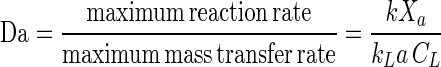6

where k_La is the mass transfer rate coefficient (per hour). If Da is ≪1, then the system is reaction rate limited, and if Da is ≫1, the system is mass transfer limited (2).

The biomass concentration decreases due to TCE transformation product toxicity (1, 8), and the mass of cells inactivated is proportional to the mass of TCE transformed

7

where T_C is the TCE transformation capacity (in grams of TCE per gram of active cells) (1).

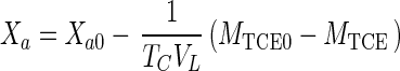
Equations 1, 4, 5, and 7 can be combined to eliminate C_G, C_L, and X_a and can be integrated (when Da is ≪1) to obtain the integrated Monod equation for cometabolism of TCE (a volatile nongrowth substrate with transformation product toxicity)

8

Equation 8 can also be applied to the simpler case of nonvolatile substrates by setting H_C equal to zero.

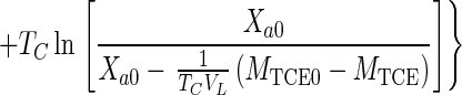
The best estimates of the rate coefficients, such as k and K_S, or other constants, such as C_L0, can be determined by comparing model predictions to observed values of C_L (or M) and t by using the known values for Y, V_L, V_G, H_C, etc., together with initial estimates of the coefficients that are sought in equation 3 or 8. The rate coefficients and other constants estimated by fitting the integrated Monod equation to experimental data are referred to as model fitting parameters. The estimates of the parameters are successively revised through trial and error or other more sophisticated searching techniques (9) to minimize the sum of the squared weighted errors (SSWE)

9

where w_i is an appropriate weighting factor, t_i^obs is the time of the ith observation, and t_i^pred is the t value predicted by the model for the measured C_L value, of C_Li^obs.

Ideally, it would be desirable to minimize the differences between the measured and predicted C_L values (C_Li^obs − C_Li^pred) because the errors in the measurement of C_L are generally much larger than the errors in the measurement of t. However, for implicit equations, such as equations 3 and 8, only the differences between predicted and observed t values (t_i^obs − t_i^pred) can be calculated explicitly. The differences between predicted and observed C_L values can be estimated by multiplying t_i^obs − t_i^pred by the local slope of the substrate disappearance curve, ΔC_L/Δt. Therefore, we propose that the logical weighting factor is the local slope of the substrate disappearance curve

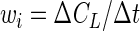10

Given this weighting factor, the quantity w_i(t_i^obs − t_i^pred) in equation 9 is

11

which is the error in the predicted C_Li^obs. This approach provides an explicit approximate method to minimize C_Li^obs − C_Li^pred in lieu of an explicit expression for C_L as a function of t.

Uncertainty in fitted parameters.

The uncertainties in the best estimates of the model parameters can be evaluated by an approximate method similar to that described elsewhere for numerical modeling applications (4, 12).

The mean square error (MSE) of a fitting parameter, which is used to calculate the 95% confidence interval of a given parameter estimate, is calculated from the mean square fitting error and the sensitivity of the model to the parameter. In general, the parameter uncertainty increases with the mean square fitting error and decreases with increasing sensitivity to the parameter.

The mean square fitting error is

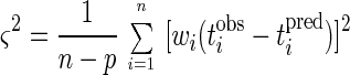12

where n is the number of observations and p is the number of parameters being determined.

The model sensitivity to the parameters is evaluated by calculating approximate first derivatives of the model predictions with respect to the parameters. Two sets of model predictions are compared, in which one parameter is varied by a small step. The sensitivity coefficient for the fitting parameter θ is evaluated at each observation as follows

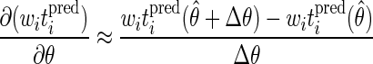13

where θ̂ is the best estimate of θ, θ̂ + Δθ is a nearby value of θ, and w_it_i^pred(θ̂) and w_it_i^pred(θ̂ + Δθ) are the weighted predictions for the times corresponding to an observed substrate concentration for the θ values θ̂ and θ̂ + Δθ, respectively. Note that although the model predictions are not compared to the observations in these calculations, the two sets of model predictions are evaluated at the points corresponding to the observations. Therefore, if the experimental observations are made at substrate concentrations that are sensitive to the model parameters, high accuracy of parameter estimates can be ensured.

In cases with only one fitting parameter, the MSE of the parameter is

14

where the denominator contains the sensitivity coefficients, squared and summed over all observations.

The square root of the MSE is the standard deviation, and the approximate 95% confidence interval for θ [(θ)_95%] is

15

For cases involving more than one fitting parameter, the sensitivity of the model predictions to the parameters is represented by a p × p matrix, A, where p is the number of fitting parameters. Such a matrix is given in equation 16 for the case involving two parameters, such as θ₁ and θ₂. The diagonal elements of the matrix (e.g., A₁₁ and A₂₂) are the sensitivity coefficients for the individual parameters, squared and summed over all observation times. The off-diagonal elements (i.e., A₁₂ and A₂₁) are products of the sensitivity coefficients for pairs of the parameters, summed over all observation times.

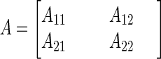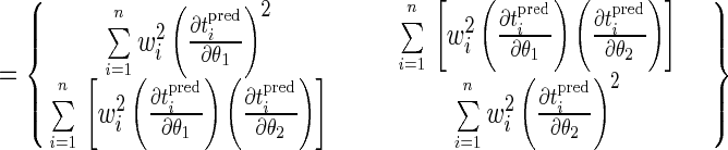16

The single-parameter standard error for each parameter can be calculated from the diagonal elements of the MSE matrix, V, which is related to the sensitivity matrix as follows

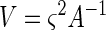17

where ς² is given by equation 12 and A⁻¹ is the inverse of A. The inverse of a matrix can be calculated by using the MINVERSE function in Microsoft Excel (Microsoft Corp., Redmond, Wash.). The standard error of θ₁, for example, is . The off-diagonal elements of V can be used to compute the correlation coefficients of the estimation error. The correlation coefficient of θ₁ and θ₂ is V₁₂/.

The single-parameter 95% confidence interval of θ₁ [(θ₁)_95%] is

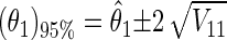18

The single-parameter confidence intervals should be used with caution because they do not reflect the joint variability of all of the fitting parameters. Joint confidence regions are more informative.

The joint confidence region, which contains the set of parameters with a probability of 95%, is the interior of an ellipse for the case with two parameters. It is the region where values of the variables θ₁ and θ₂ satisfy the inequality

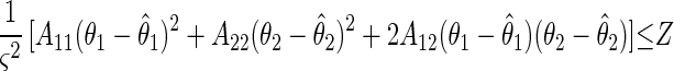19

where θ̂₁ and θ̂₂ are the best estimates of the parameters. The value of Z is based on the F distribution for finite sample sizes and is a function of the numbers of observations and parameters and the selected confidence interval probability as follows

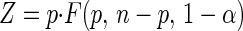20

where F(p, n-p, 1-α) is taken from an F-distribution table (4) and 1-α is the fractional probability (0.95 for the 95% probability case) (4). The joint 95% confidence region can be plotted with the Goal Seek function in Excel by entering θ₁ values and using Goal Seek to find θ₂ values that satisfy equation 19. Alternatively, a graphics program with a contour plotting function, such as Mathematica, can be used.

RESULTS

Application. (i) Acetate utilization.

Experimental data for acetate utilization by a methanogenic mixed culture at 25°C (7) were analyzed to determine the rate coefficients k and K_S and the initial substrate concentration C_L0 by fitting equation 3 to acetate utilization rate data by using a computer spreadsheet and weighted nonlinear least-squares analysis (equations 9 and 10). C_L0 was used as a fitting parameter because it was not known with greater certainty than the other data points and it would not be appropriate to force the best-fit curve through the measured value of C_L0. The input value for Y was determined in separate experiments, and X_a0 was estimated based on the combined results of several experiments. All of the calculations were done on an Apple Macintosh computer (Apple Computer, Cupertino, Calif.) by using a spreadsheet program (Microsoft Excel 4.0). The joint 95% confidence regions were plotted with Mathematica 2.2 for Macintosh (Wolfram Research Inc., Champaign, Ill.).

An example of a spreadsheet for fitting the integrated Monod equation to the data is shown in Table 1. The values of the rate coefficients and other constants, some of which were used as fitting parameters, are given in rows 1 through 5. The values of the fitting parameters shown were initial guesses that were subsequently changed by the program as the model was fitted to the experimental data. The experimental data are listed in columns A and B, in order of decreasing C_L. Column C contains the calculated t value for each observed C_L value (equation 3). The calculated values are shown in Table 1 rather than the equations. Column D contains the C_L values used to calculate the values in column C. These C_L values are the same as the values in column B except for the first value, which is a variable fitting parameter. The biomass concentrations were calculated (column E) but were not required for the purpose of curve fitting. Additional model predictions used to calculate the weighting factors are shown in columns F and G; the C_L values in column G are slightly lower (0.1 mg/liter lower) than the values in column D, and the t values in column F were calculated from the values in column G by using equation 3. Column H shows the local slope of the model curve, which was calculated for each observation by using the two sets of model predictions; for example, the value at H11 (column H, row 11) equals (D11−G11)/(C11−F11). The differences between model and predicted t values (column A − column C) were calculated (column I), and the results were multiplied by the weighting factors (column H) to give the weighted errors (column J). The weighted errors were squared (column K), and the squared weighted errors were summed (cell K36).

TABLE 1.

Example spreadsheet for fitting the integrated Monod equation to acetate utilization rate data^a

^ad, day; L, liter. 

The model was fitted to the data by using the Solver function under the Formula menu in Excel to adjust the parameter estimates to minimize the SSWE (cell K36). The best fit was obtained with Solver, which uses an iterative search for the parameter values that yielded the minimum SSWE, and the initial estimates of the parameters were automatically replaced by the best estimates in rows 2, 3, and 5. Solver can search quickly for a maximum, minimum, or specified value for any selected cell by varying the values for one or more other selected cells in a spreadsheet. It is also possible to define limits for the values of the variables, such as K_S > 0, if Solver gives unrealistic results.

The best estimates of the rate coefficients k (7.4 day⁻¹) and K_S (23.2 mg/liter), obtained from fitting equation 3 to the data set in which the C_L0 value was 50 mg/liter, yielded a model curve that is an excellent fit to all three data sets shown in Fig. 1. Since the data were obtained from mixed-culture experiments, these rate coefficients represent the overall values for the different organisms present and may not be directly comparable to other previously published values.

FIG. 1.

Results of fitting the integrated Monod equation to acetate utilization rate data by using the weighted nonlinear least-squares spreadsheet method. The model (heavy solid line) was fitted to one data set (□), which resulted in the following values: k = 7.4 day⁻¹, K_S = 23.2 mg/liter, and C_L0 = 53.5 mg/liter. Model curves obtained with the same k and K_S values are shown for other data (Δ and ○) for comparison. L, liter; d, day.

Only one data set was used to estimate the rate coefficients. The resulting values for the coefficients were used to generate the two additional curves for comparison with the other two data sets (C_L0 was used as the first data point for the two additional curves). The two data sets obtained with lower initial acetate concentrations (Fig. 1) were not very sensitive to the parameters because C_L was less than K_S throughout the experiments, and therefore, these data did not add much information about the parameters k and K_S. If all three data sets were used in the parameter fitting procedure with five fitting parameters (k, K_S, and a C_L0 value for each experiment), the estimation accuracy would not improve. Robinson (9) gives a very good explanation of experimental design and substrate concentrations that yield data that are sensitive to the parameters of interest.

The uncertainty calculations were performed by using additional spreadsheet calculations not shown in Table 1. The mean square fitting error was calculated from the SSWE value in cell K36 and the n and p values (25 data points and 3 parameters, respectively) by using equation 12. The sensitivity coefficients for each parameter were determined by calculating a new set of model points by using the best estimates of all fitting parameters except the parameter of interest, which was varied by a small increment. The sensitivity coefficient was evaluated at each point by using equation 13, and the individual values were squared and summed for use in equation 14 or for the diagonal elements of the matrix in equation 16. The off-diagonal elements of equation 16 were calculated by summing the products of the individual sensitivity values. The resulting sensitivity coefficients obtained in equation 16 were used in the equation for the 95% confidence region, equation 19.

Since three fitting parameters were used in this case, the joint 95% confidence region was a three-dimensional ellipsoid which represented the region containing k, K_S, and C_L0 with a probability of 95%. Three slices of this ellipsoid are shown in Fig. 2. The slices were taken in the plane C_L0 = Ĉ_L0 and C_L0 = Ĉ_L0 ± ς_CL0, where Ĉ_L0 is the best estimate of C_L0 and ς_CL0 is the standard error of C_L0, as defined in Materials and Methods. There were no points in the plane C_L0 = Ĉ_L0 ± 2 ς_CL0 due to the low correlation of uncertainty between C_L0 and the other two parameters.

FIG. 2.

Joint 95% confidence region for k and K_S for the data in Fig. 1. Slices of the three-dimensional ellipsoid were taken along the C_L0 axis at Ĉ_L0 (large ellipse) and Ĉ_L0 ± ς_CL0 (small ellipse; there were two ellipses, but they had the same size and location). L, liter; d, day.

(ii) TCE cometabolism.

TCE cometabolism rate data were obtained from batch experiments performed with resting cells (no methane or other carbon or energy source was present) in a mixed culture that were transforming TCE. The apparatus was a closed 2-liter vessel with a headspace present to provide oxygen from air and for the convenience of headspace analysis of TCE. The methods are described in detail elsewhere (12). Gas-liquid equilibrium was verified by mass transfer rate measurements. After the reaction was started by adding cells, the disappearance of TCE was monitored by periodically measuring the TCE in the headspace and calculating the TCE mass present (M_i^obs) (Fig. 3). The experimental methods used are described elsewhere (12).

FIG. 3.

Comparison of model fits for TCE cometabolism data. Parameter estimates were obtained by using the integrated Monod equation (——), the numerical model (— —), and the numerical model with simplifying assumptions (–––). Two of the curves are shown with the same symbol, because they are indistinguishable at the scale of this graph.

The integrated Monod equation for a nongrowth substrate with product toxicity (equation 8) was fitted to the data in Fig. 3. For this data set, it was not possible to obtain unique estimates for k_TCE and K_S,TCE by using the spreadsheet model because the coefficients were highly correlated. Many pairs of k_TCE and K_S,TCE values that yielded a k_TCE/K_S,TCE ratio of 0.31 liter/mg/day were found that had SSWE values very near the same minimum value. Therefore, the k_TCE/K_S,TCE ratio was used as a fitting parameter as an alternative approach. The k_TCE/K_S,TCE and T_C values were varied by Solver until the minimum SSWE was found. The k_TCE/K_S,TCE value was varied by leaving the k_TCE value fixed and allowing Solver to vary the K_S,TCE value. As shown in Fig. 3, the spreadsheet fitting method gave a model curve that is an excellent fit to the data. As stated above for the acetate utilization data, these results for mixed cultures represent overall rates for several organisms and might not be directly comparable to other previously published values.

In order to test the reliability of this method, the best estimates and joint 95% confidence regions obtained from the integrated Monod spreadsheet analysis were compared to estimates and confidence regions obtained by fitting a more rigorous numerical model to the data (12). The numerical model used included a fourth-order Runge-Kutta solution for the system of differential equations describing the experimental conditions, including Monod kinetics, changes in active organism concentration due to product toxicity and endogenous decay, gas-liquid mass transfer of TCE, and passive losses of TCE from the apparatus. The numerical model calculated fitting errors (M_i^obs − M_i^pred)² at the times corresponding to each data point.

The estimates of k_TCE/K_S,TCE and T_C values obtained by using the integrated Monod spreadsheet analysis method were not significantly different than those obtained by using the more rigorous numerical model, as shown in Table 2 and Fig 3 and 4. For both models, it was assumed that the initial concentration of active organisms was equal to 20% of the initial total suspended-solids concentration, based on the results of methane utilization rate experiments and modeling results obtained with the mixed culture, as described previously (12).

TABLE 2.

Best estimates, approximate 95% confidence intervals, and correlation coefficients for TCE cometabolism rate data shown in Fig. 3

TCE cometabolism rate coefficient	Best estimate of previous numerical modela	Present study
		Best estimate of numerical model assuming no cell decay and no TCE losses	Integrated Monod equation weighted least-squares analysis
			Best estimate	Correlation coefficients
				k/KS	TC
k/KS (liter/mg/day)	0.35 ± 0.08	0.35 ± 0.08	0.31 ± 0.06	1
TC (g/g)	0.21 ± 0.03	0.23 ± 0.02	0.23 ± 0.02	−0.63	1

^aData from reference 12. 

FIG. 4.

Joint 95% confidence regions for k_TCE/K_S,TCE and T_C for the TCE cometabolism results shown in Fig. 3, using the numerical model (— – —), the numerical model with simplifying assumptions (—), and integrated Monod equation weighted least-squares analysis (–––). L, liter; d, day.

The most significant differences between the numerical model and the integrated Monod equation weighted least-squares approach are the error calculation methods and the assumptions regarding TCE losses, endogenous decay of the organisms, and gas-liquid equilibrium. The TCE losses and endogenous decay were neglected, and gas-liquid equilibrium was assumed in the integrated Monod equation approach because the equation cannot be integrated if these processes are included. In many cases, such assumptions are justified. The dissolved TCE concentrations predicted by the numerical model were within 1% of the equilibrium concentrations, and therefore it was known a priori that the equilibrium assumption was valid for this data set. Justification for this assumption would be necessary in other applications of this approach.

In order to compare the two models more directly, the numerical model was fitted to the data assuming that there were no TCE losses from the reactor and there was no endogenous cell decay (Table 2). A comparison of the estimates in Table 2 indicates that the assumption concerning no TCE losses and the different methods of error calculations had only slight effects, while the assumption that there was no endogenous decay had an insignificant effect on the analysis of this data set. The integrated Monod equation weighted least-squares analysis and numerical model with simplifying assumptions yielded a higher T_C estimate than the complete numerical model because all of the TCE removed was considered biodegraded in the former two cases, which yielded a higher T_C estimate than the numerical model, which correctly accounted for the TCE removal due to passive losses. The estimated k_TCE/K_S,TCE value obtained from the integrated Monod equation weighted least-squares approach was somewhat lower, although the difference was not statistically significant. The slight difference was due to the different methods of calculating fitting errors and was verified by comparing the calculated SSWE (equation 9) for both k_TCE/K_S,TCE estimates with the true errors, , calculated by trial and error application of equation 8 for each k_TCE/K_S,TCE estimate.

The integrated Monod equation weighted least-squares analysis method is a good approximation of the more rigorous numerical model for this data set because the best estimates of each model were within the bounds of the joint 95% confidence region of the other model (Fig. 4). The differences in the estimates for the rate coefficient ratio shown in Table 2 and discussed above are not statistically significant, but they do illustrate the differences between the modeling techniques. It is important to recognize that under other conditions, such as experimental runs of more than 1 day, passive TCE losses and endogenous decay are likely to be more significant, and the integrated Monod equation weighted least-squares approach might then not provide reliable estimates of the rate coefficients.

DISCUSSION

The integrated Monod equation method is a simple procedure for obtaining reliable estimates of microbiological reaction rate coefficients as long as the requirements of the underlying assumptions are met. The fraction of cells lost over the course of the experiment due to endogenous decay of cells must be small. Changes in cell concentration due to growth or product toxicity do not limit the applicability of this method because they can be included in the integrated form of the equation. For volatile substrates, the experimental system must be at gas-liquid equilibrium and the rate of passive loss of substrates, such as TCE, must be low relative to the transformation rate.

The weighting method described in this paper has a rational statistical basis. The difference between the observed and predicted substrate concentrations is estimated by multiplying the slope of the substrate disappearance curve by the difference between measured and predicted sample times. This approach is appropriate because it approximates the error in the measurement of substrate concentration and such errors are usually larger than errors in time measurement in biochemical rate experiments.

The use of linearized forms of the Monod equation, such as Lineweaver-Burk and Eadie-Hofstee plots, should be avoided because several critical assumptions of linear regression are violated by these methods, which leads to inaccurate parameter estimates and a lack of any way to evaluate the uncertainties in the parameter estimates (9). Because of the availability of computers and software that are easy to use, the use of linearized approaches is no longer justified. The weighted nonlinear least-squares method described in this paper is very straightforward and easy to apply with a computer spreadsheet program.

Another important advantage of the integrated Monod equation method over linearized methods is the economy of obtaining rate coefficients from a single batch experiment or a few batch experiments rather than having to obtain large numbers of initial rate measurements. However, the uncertainty calculations from a single experiment do not reflect the run-to-run variability in parameter estimates. When initial rate measurements are used, the rate coefficients and their uncertainties can be determined more precisely from nonlinear least-squares analysis (e.g., applied to a plot of −dC_L/dt versus C_L) than from linearized plots of inverted data.

Statistical software packages for personal computers may also allow convenient application of the integrated Monod equation if they provide for weighting in the nonlinear least-squares fitting and uncertainty analysis. In the absence of a weighting factor, a nonlinear least-squares approach would minimize the differences between measured and predicted t values rather than C_L values, which would be inappropriate for an implicit expression, such as the integrated Monod equation. Users should be careful not to use nonlinear least-squares fitting software without appropriate provisions, such as a weighting factor, when they use implicit equations, such as the integrated Monod equation.

Comparison with a rigorous numerical model validated the results obtained by the integrated Monod equation spreadsheet method. One important advantage of the integrated Monod equation spreadsheet method over a numerical model is the flexibility that it offers to use the initial substrate concentration as a fitting parameter, which is desirable when the initial substrate concentration data point is known with certainty equal to that of all other data points.

Rate experiments can be designed to maximize the informative value of the results. Coefficients, such as Y, that are measured separately and used as constants in the parameter fitting process should be measured as accurately as possible. Accurate measurements of other constants, such as the initial active biomass concentration, are crucial for minimizing the uncertainties in the fitted parameters. The number of fitting parameters should be minimized, and the concentrations of biomass and substrate should be selected to yield the most information about the rate parameters of interest. The use of sensitivity analysis to design experiments has been described by Robinson (9).

The method described above for calculating the uncertainties in rate coefficients makes great use of the information available from the data without requiring the use of sophisticated mathematics. When the initial substrate concentration is not used as a fitting parameter, this method can be used to describe a confidence region precisely based on numerous data sets if desired. However, when the initial substrate concentration is used as a fitting parameter, each data set included in the analysis adds one fitting parameter, and both the fitting calculations and the graphical representation of the confidence region become difficult with three or more data sets. In this situation, it may be preferable to use the fitting technique described in this paper to determine the best-fit value of each rate coefficient for each experiment and use the mean and standard deviation of the best-fit values from all of the experiments to evaluate the confidence interval for each rate coefficient.

Copies of the spreadsheet are available on diskette from the corresponding author.

REFERENCES

- 1.Alvarez-Cohen L, McCarty P L. A cometabolic biotransformation model for halogenated aliphatic compounds exhibiting product toxicity. Environ Sci Technol. 1991;25:1381–1387. [Google Scholar]
- 2.Bailey J E, Ollis D F. Biochemical engineering fundamentals. New York, N.Y: McGraw-Hill Book Company; 1986. [Google Scholar]
- 3.Dowd J E, Riggs D S. A comparison of estimates of Michaelis-Menten kinetic constants from various linear transformations. J Biol Chem. 1965;240:863–869. [PubMed] [Google Scholar]
- 4.Draper N R, Smith H. Applied regression analysis. New York, N.Y: John Wiley & Sons; 1981. [Google Scholar]
- 5.Eisenthal R, Cornish-Bowden A. The direct linear plot: a new graphical procedure for estimating enzyme kinetic parameters. Biochem J. 1974;139:715–720. doi: 10.1042/bj1390715. [DOI] [PMC free article] [PubMed] [Google Scholar]
- 6.Hanes C S. Studies on plant amylases. I. The effect of starch concentration upon the velocity of hydrolysis by the amylase of germinated barley. Biochem J. 1932;26:1406–1421. doi: 10.1042/bj0261406. [DOI] [PMC free article] [PubMed] [Google Scholar]
- 7.Montgomery M S. Kinetics of methane fermentation in anaerobic biofilms. Ph.D. thesis. Stanford, Calif: Stanford University; 1983. [Google Scholar]
- 8.Oldenhuis R, Oedzes J Y, van der Waarde J J, Janssen D B. Kinetics of chlorinated hydrocarbon degradation by Methylosinus trichosporium OB3b and toxicity of trichloroethylene. Appl Environ Microbiol. 1991;57:7–14. doi: 10.1128/aem.57.1.7-14.1991. [DOI] [PMC free article] [PubMed] [Google Scholar]
- 9.Robinson J A. Determining microbial kinetic parameters using nonlinear regression analysis. Adv Microb Ecol. 1985;8:61–114. [Google Scholar]
- 10.Robinson J A, Charaklis W G. Simultaneous estimation of Vmax, Km, and the rate of endogenous substrate production (R) from substrate depletion data. Microb Ecol. 1984;10:165–178. doi: 10.1007/BF02011423. [DOI] [PubMed] [Google Scholar]
- 11.Sawyer C N, McCarty P L, Parkin G F. Chemistry for environmental engineering. New York, N.Y: McGraw-Hill, Inc.; 1994. [Google Scholar]
- 12.Smith L H, Kitanidis P K, McCarty P L. Numerical modeling and uncertainties in rate coefficients for methane utilization and TCE cometabolism by a methane-oxidizing mixed culture. Biotechnol Bioeng. 1997;53:320–331. doi: 10.1002/(SICI)1097-0290(19970205)53:3<320::AID-BIT11>3.0.CO;2-O. [DOI] [PubMed] [Google Scholar]