Statistics review 12: Survival analysis

Abstract

This review introduces methods of analyzing data arising from studies where the response variable is the length of time taken to reach a certain end-point, often death. The Kaplan–Meier methods, log rank test and Cox's proportional hazards model are described.

Introduction

Survival times are data that measure follow-up time from a defined starting point to the occurrence of a given event, for example the time from the beginning to the end of a remission period or the time from the diagnosis of a disease to death. Standard statistical techniques cannot usually be applied because the underlying distribution is rarely Normal and the data are often 'censored'. A survival time is described as censored when there is a follow-up time but the event has not yet occurred or is not known to have occurred. For example, if remission time is being studied and the patient is still in remission at the end of the study, then that patient's remission time would be censored. If a patient for some reason drops out of a study before the end of the study period, then that patient's follow-up time would also be considered to be censored.

The hypothetical data set given in Table 1 will be used for illustrative purposes in this review. For this data set the event is the death of the patient, and so the censored data are those where the outcome is survived or unknown.

Table 1.

Survival time, age and outcome for a group of patients diagnosed with a disease and receiving one of two treatments

Patient number	Survival time (days)	Outcome	Treatment	Age (years)
1	1	Died	2	75
2	1	Died	2	79
3	4	Died	2	85
4	5	Died	2	76
5	6	Unknown	2	66
6	8	Died	1	75
7	9	Survived	2	72
8	9	Died	2	70
9	12	Died	1	71
10	15	Unknown	1	73
11	22	Died	2	66
12	25	Survived	1	73
13	37	Died	1	68
14	55	Died	1	59
15	72	Survived	1	61

Estimating the survival curve using the Kaplan–Meier method

In analyzing survival data, two functions that are dependent on time are of particular interest: the survival function and the hazard function. The survival function S(t) is defined as the probability of surviving at least to time t. The hazard function h(t) is the conditional probability of dying at time t having survived to that time.

The graph of S(t) against t is called the survival curve. The Kaplan–Meier method can be used to estimate this curve from the observed survival times without the assumption of an underlying probability distribution. The method is based on the basic idea that the probability of surviving k or more periods from entering the study is a product of the k observed survival rates for each period (i.e. the cumulative proportion surviving), given by the following:

S(k) = p₁ × p₂ × p₃ × ... × p_k

Here, p₁ is the proportion surviving the first period, p₂ is the proportion surviving beyond the second period conditional on having survived up to the second period, and so on. The proportion surviving period i having survived up to period i is given by:

Where r_i is the number alive at the beginning of the period and d_i the number of deaths within the period.

To illustrate the method the data for the patients receiving treatment 2 from Table 1 will be used. The survival times, including the censored values (indicated by + in Table 2), must be ordered in increasing duration. If a censored time has the same value as an uncensored time, then the uncensored should precede the censored. The calculations are shown in Table 2. Where there is a censored time the proportion surviving will be 1. This does not alter the cumulative proportion surviving, and so these calculations can be omitted from the table. For more detailed explanation, see Swinscow and Campbell [1].

Table 2.

Calculations for the Kaplan–Meier estimate of the survival function for the treatment 2 data from Table 1

Patient number	Survival time (days)	Number known to be alive (ri)	Deaths (di)	Proportion surviving (pi)	Cumulative proportion surviving (S [t])
	0				1
1	1	8
2	1	8	2	(8 - 2)/8 = 0.750	1 × 0.750 = 0.750
3	4	6	1	(6 - 1)/6 = 0.833	0.750 × 0.833 = 0.625
4	5	5	1	(5 - 1)/5 = 0.800	0.625 × 0.800 = 0.500
5	6+
7	9	3	1	(3 - 1)/3 = 0.667	0.500 × 0.667 = 0.333
8	9+
11	22	1	1	(1 - 1)/1 = 0.00	0.333 × 0.00 = 0.000

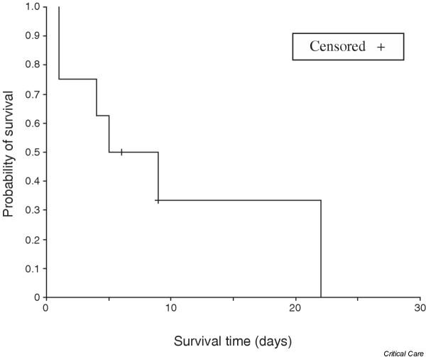
Plotting the cumulative proportion surviving against the survival times gives the stepped survival curve shown in Fig. 1.

Figure 1.

Plot of the survival curve for treatment 2.

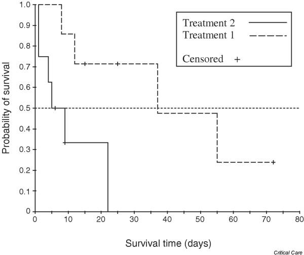
This method is found in most statistical packages. Figure 2 is the output from a statistical package used to compare the survival curves for the two treatment groups for the data given in Table 1.

Figure 2.

Survival curves for the two treatment groups for the data in Table 1.

It can be seen that patients on treatment 1 appear to have a higher survival rate than those on treatment 2. The graph can be used to estimate the median survival time because this is the time with probability of survival of 0.5. The median survival time for those on treatment 2 appears to be 5 days versus about 37 days on treatment 1.

Comparing survival curves of two groups using the log rank test

Comparison of two survival curves can be done using a statistical hypothesis test called the log rank test. It is used to test the null hypothesis that there is no difference between the population survival curves (i.e. the probability of an event occurring at any time point is the same for each population). The test statistic is calculated as follows:

Where the O₁ and O₂ are the total numbers of observed events in groups 1 and 2, respectively, and E₁ and E₂ the total numbers of expected events.

The total expected number of events for a group is the sum of the expected number of events at the time of each event. The expected number of events at the time of an event can be calculated as the risk for death at that time multiplied by the number alive in the group. Under the null hypothesis, the risk of death (number of deaths/number alive) can be calculated from the combined data for both groups. Table 3 shows the calculation of the expected number of deaths for treatment group 2 for the example data. For example, at the beginning of day 4 when the third death (event 3) takes place, there are 13 patients still alive. One dies, giving a risk for death of 1/13 = 0.077. Six of the 13 patients are from treatment group 2, and therefore the expected number of deaths is given by 6 × 0.077 = 0.46 at event 3. The total expected number of events for group 2 is calculated as:

Table 3.

Calculations for the log-rank test to compare treatments for the data in Table 1

Survival time (days)	Treatment group	Number known to be alive (ri)	Deaths (di)	Risk for death (di/ri)	Number known to be alive from treatment group 2 (r2i)	Expected number of events in treatment group 2 (E2i)
0
1	2	15	2	2/15 = 0.133	8	8 × 0.133 = 1.07
1	2
4	2	13	1	1/13 = 0.077	6	6 × 0.077 = 0.46
5	2	12	1	1/12 = 0.083	5	5 × 0.083 = 0.42
6+	2	11	0	0/11 = 0	4	4 × 0 = 0.00
8	1	10	1	1/10 = 0.100	3	3 × 0.100 = 0.30
9	2	9	1	1/9 = 0.111	3	3 × 0.111 = 0.33
9+	2	8	0	0/8 = 0	2	2 × 0 = 0.00
12	1	7	1	1/7 = 0.143	1	1 × 0.143 = 0.14
15+	1	6	0	0/6 = 0	1	1 × 0 = 0.00
22	2	5	1	1/5 = 0.200	1	1 × 0.200 = 0.20
25+	1	4	0	0/4 = 0	0	0 × 0 = 0.00
37	1	3	1	1/3 = 0.333	0	0 × 0 = 0.00
55	1	2	1	1/2 = 0.500	0	0 × 0 = 0.00
72+	1
						E2 = 2.92

Where r_2i is the number alive from group 2 at the time of event i. E₁ can be calculated as n - E₂, where n is the total number of events.

The test statistic is compared with a χ² distribution with 1 degree of freedom. It is a simplified version of a statistic that is often calculated in statistical packages [2].

For the data in Table 1, the total number of expected deaths for treatment group 2 is calculated as 2.92 and the total number of observed deaths is 10, giving a total number of expected deaths for treatment group 1 of 10 - 2.92 = 7.08. The value of the test statistic is therefore calculated as follows:

This gives a P value of 0.032, which indicates a significant difference between the population survival curves.

An assumption for the log rank test is that of proportional hazards. This is discussed below. Small departures from this assumption, however, do not invalidate the test.

Cox's proportional hazards model (Cox regression)

The log rank test is used to test whether there is a difference between the survival times of different groups but it does not allow other explanatory variables to be taken into account.

Cox's proportional hazards model is analogous to a multiple regression model and enables the difference between survival times of particular groups of patients to be tested while allowing for other factors. In this model, the response (dependent) variable is the 'hazard'. The hazard is the probability of dying (or experiencing the event in question) given that patients have survived up to a given point in time, or the risk for death at that moment.

In Cox's model no assumption is made about the probability distribution of the hazard. However, it is assumed that if the risk for dying at a particular point in time in one group is, say, twice that in the other group, then at any other time it will still be twice that in the other group. In other words, the hazard ratio does not depend on time.

The model can be written as:

Where h(t) is the hazard at time t; x₁, x₂... x_p are the explanatory variables; and h₀(t) is the baseline hazard when all the explanatory variables are zero. The coefficients b₁, b₂ ... b_p are estimated from the data using a statistical package.

Because hazard measures the instantaneous risk for death, it is difficult to illustrate it from sample data. Instead, the cumulative hazard function H(t) can be examined. This can be obtained from the cumulative survival function S(t) as follows:

H(t) = -ln S(t)

The estimated cumulative hazard function for the example data given in Table 1 is shown in Table 4.

Table 4.

Cumulative hazard functions (logarithmic scale) for the example data

Survival time (days): t	Cumulative survival: S(t)	Cumulative hazard: H(t) = -ln S(t)
Treatment 1
8	0.8571	0.1542
12	0.7143	0.3365
15	0.7143	0.3365
25	0.7143	0.3365
37	0.4762	0.7419
55	0.2381	1.4351
72	0.2381	1.4351
Treatment 2
1
1	0.7500	0.2877
4	0.6250	0.4700
5	0.5000	0.6931
6	0.5000	0.6931
9	0.5000	0.6931
9	0.3333	1.0986
22	0.0000

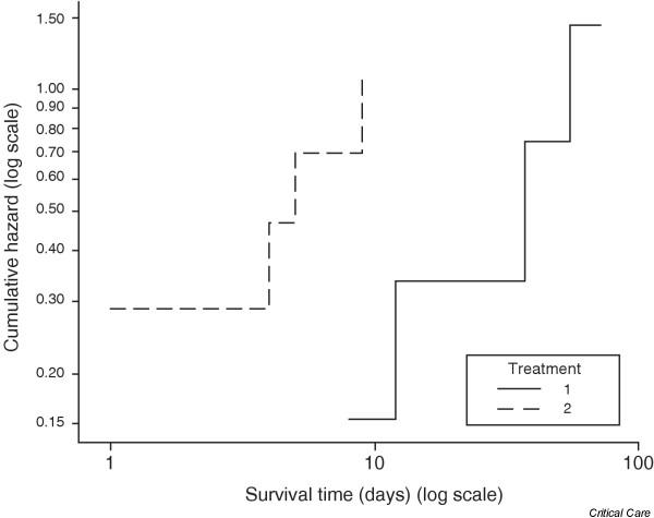
The assumption that the proportional hazards stay constant over time can be inspected by looking at a graph showing the logarithm of the estimated cumulative hazard function. The assumption is equivalent to assuming that the difference between the logarithms of the hazards for the two treatments does not change with time, or equally that the difference between the logarithms of the cumulative hazard functions is constant. Figure 3 is the graph for the example data. The lines for the two treatments are roughly parallel, suggesting that the proportional hazards assumption is reasonable in this case. A more formal test of the assumption is possible (see Armitage and coworkers [2]). Note that, in this graph, the time scale was also logarithmically transformed. This was to make the comparison clearer between the two treatments, but it does not affect the vertical positioning of the lines.

Figure 3.

Cumulative hazard functions for the example data.

Cox's regression was applied to the example data using treatment and age as explanatory variables. The output is shown in Table 5.

Table 5.

Application of Cox's regression to the example data, using treatment and age as explanatory variables

	Coefficient (b)	Standard error	P	eb	95.0% confidence interval for eb
Treatment	-1.887	0.973	0.052	0.152	0.022–1.020
Age	0.220	0.085	0.010	1.247	1.054–1.474

The P values indicate that the difference between treatments was bordering on statistical significance, whereas there was strong evidence that age was associated with length of survival. The coefficient for treatment, -1.887, is the logarithm of the hazard ratio for a patient given treatment 1 compared with a patient given treatment 2 of the same age. The exponential (antilog) of this value is 0.152, indicating that a person receiving treatment 1 is 0.152 times as likely to die at any time as a patient receiving treatment 2; that is, the risk associated with treatment 1 appears to be much lower. However, the confidence interval contains 1, indicating that there may be no difference in risk associated with the two treatments.

Using the Kaplan–Meier (log rank) test, the P value for the difference between treatments was 0.032, whereas using Cox's regression, and including age as an explanatory variable, the corresponding P value was 0.052. This is not a substantial change and still suggests that a difference between treatments is likely. In this case age is clearly an important explanatory variable and should be included in the analysis.

The exponential of the coefficient for age, 1.247, indicates that a patient 1 year older than another patient, both being given the same treatment, has an increased risk for dying, by a factor of 1.247. Note that, in this case, the confidence interval does not contain 1, indicating the statistical significance of age.

Further models for survival data, allowing for different assumptions, are discussed by Kirkwood and Sterne [3].

An example from the literature

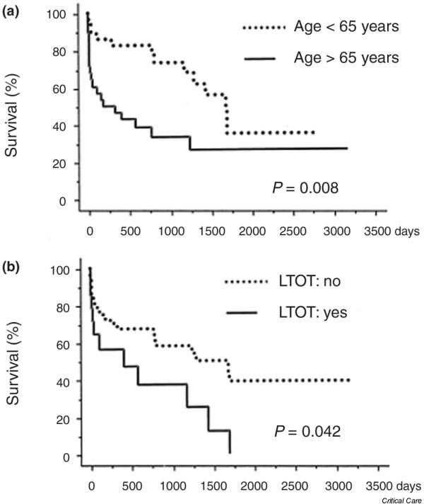
Dupont and coworkers [4] investigated the survival of patients with bronchiectasis according to age and use of long-term oxygen therapy. The Kaplan–Meier curves and results of the log rank tests shown in Fig. 4 indicate that there is a significant difference between the survival curves in each case.

Figure 4.

The Kaplan–Meier estimates of survival for (a) age > 65 years or ≤ 65 years, and (b) long-term oxygen therapy (LTOT) before intensive care unit admission (yes/no). The P values are for the log rank test.

The authors also applied Cox's proportional hazards analysis and obtained the results given in Table 6. These results indicate that both age and long-term oxygen therapy have a significant effect on survival. The estimated risk ratio for age, for example, suggests that the risk for death for patients over the age of 65 years is 2.7 times greater than that for those below 65 years.

Table 6.

Results of Cox's proportional hazards analysis for the patients with bronchiectasis

Explanatory variables	Risk ratio	95% confidence interval	P
Age (>65 years)	2.7	1.15–6.29	0.022
LTOT (yes)	3.12	1.47–6.90	0.003

LTOT, long-term oxygen therapy.

Assumptions and limitations

The log rank test and Cox's proportional hazards model assume that the hazard ratio is constant over time. Care must be taken to check this assumption.

Conclusion

Survival analysis provides special techniques that are required to compare the risks for death (or of some other event) associated with different treatments or groups, where the risk changes over time. In measuring survival time, the start and end-points must be clearly defined and the censored observations noted. Only the most commonly used techniques are introduced in this review. Kaplan–Meier provides a method for estimating the survival curve, the log rank test provides a statistical comparison of two groups, and Cox's proportional hazards model allows additional covariates to be included. Both of the latter two methods assume that the hazard ratio comparing two groups is constant over time.

Competing interests

None declared.

References

- Swinscow TDV, Campbell MJ. Statistics at Square One. London: BMJ Books; 2002. [Google Scholar]
- Armitage P, Berry G, Matthews JNS. Statistical Methods in Medical Research. 4. Oxford, UK: Blackwell Science; 2002. [Google Scholar]
- Kirkwood BR, Sterne JAC. Essential Medical Statistics. 2. Oxford, UK: Blackwell Science Ltd; 2003. [Google Scholar]
- Dupont M, Gacouin A, Lena H, Lavoue S, Brinchault G, Delaval P, Thomas R. Survival of patients with bronchiectasis after the first ICU stay for respiratory failure. Chest. 2004;125:1815–1820. doi: 10.1378/chest.125.5.1815. [DOI] [PubMed] [Google Scholar]