Fragment-based screening by protein-detected NMR spectroscopy

Abstract

Fragment-based drug discovery (FBDD) identifies low molecular weight compounds that can be developed into ligands with high affinity and selectivity for therapeutic targets. Screening fragment libraries (<10,000 molecules) with biophysical techniques against macromolecules provides information about novel chemical spaces that bind the macromolecule and scaffolds that can be modified to increase potency. A fragment-screening pipeline requires a standardized protocol for target selection, library assembly and maintenance, library screening, and hit validation to ensure hit integrity. Herein, the fundamental aspects of a fragment screening pipeline—focusing on protein-detected NMR data collection and analysis—are discussed in detail for researchers to use as a resource in their FBDD projects. Selected screening targets must undergo rigorous stability and buffer testing by NMR spectroscopy to ensure the protein structure is stable for the entire screen. Biophysical instrumentation that rapidly measures protein thermostability is helpful in buffer screening. Molecules in fragment libraries are analyzed computationally and physically, stored at appropriate temperatures, and multiplexed in well plates for library conservation. The screening protocol is streamlined using liquid handling robotics for sample preparation and customized Python scripts for protein-detected NMR data analysis. Molecules identified from the screen are titrated to determine their binding site(s) and K_d values and confirmed with an orthogonal biophysical assay. This detailed FBDD screening pipeline developed by the Program in Chemical Biology at the Medical College of Wisconsin has successfully screened many unrelated target proteins to identified novel molecules that selectively bind to these target proteins.

1. Introduction

Fragment-based drug discovery (FBDD) has emerged as a powerful approach to developing lead compounds with high affinity and selectivity toward therapeutic targets. Unlike traditional high-throughput screening, FBDD focuses on screening smaller libraries (hundreds to thousands) of low molecular weight compounds (fragments) against target proteins (Erlanson, McDowell, & O’Brien, 2004). The identified fragments typically bind with relatively weak affinity and are then elaborated into high-affinity drug candidates through iterative rounds of chemical optimization (Shuker, Hajduk, Meadows, & Fesik, 1996). Biophysical techniques that detect weak interactions are essential for FBDD since these techniques allow the detection of binding events often missed by other methods.

Among the biophysical techniques available, nuclear magnetic resonance (NMR) is well-suited for fragment screening. NMR detects binding events in a non-destructive manner for various fragment sizes, chemical properties, and relatively weak affinities (Shuker et al., 1996). While both ligand- and protein-detected NMR are used for FBDD, protein-detected NMR offers several advantages. One advantage is that the target protein is labeled with stable isotopes (¹⁵N and/or ¹³C), which allows direct observation of protein signals in the NMR spectra and direct detection of binding events rather than relying on indirect methods such as ligand-detected saturation transfer difference (STD) NMR. Another advantage is that protein-detected NMR directly determines the binding site of a fragment by measuring changes in the NMR spectra (chemical shift perturbations; CSPs) of the protein backbone or side chains, which guides subsequent optimization efforts (Zuiderweg, 2002). Protein-detected NMR can also directly determine binding affinities in the μM to low mM range by quantifying CSPs in the protein NMR spectra as a function of the fragment concentration (Fielding, 2003).

In this chapter, we provide comprehensive protocols detailing the fragment screening pipeline by protein-detected NMR that we have developed over the past eight years in the Program in Chemical Biology at the Medical College of Wisconsin, including target selection and preparation, library assembly and maintenance, screening data acquisition and analysis, and hit validation and optimization. Overall, this chapter is a practical guide for researchers interested in incorporating protein-detected NMR spectroscopy into their FBDD workflow.

2. Target selection and preparation

Fragment screening by protein-detected NMR requires significant amounts of pure, soluble target protein suitable for isotope labeling (Sheng & Zhang, 2013). NMR experiments of the protein ideally produce stable spectra where all residues are represented (except prolines) with consistent peak intensities throughout (Ziarek, Peterson, Lytle, & Volkman, 2011). Ideal target proteins are relatively small (<30 kDa) and easy to produce in standard bacterial expression systems that support uniform labeling with stable isotopes for NMR (i.e., ¹⁵N and ¹³C). This relatively small protein can be an isolated domain from a larger protein (e.g., bromodomains). In contrast, the successful application of fragment screening on membrane proteins (e.g., G-protein coupled receptors) is greatly challenged by low expression yields and issues related to solubilization while maintaining a functional structure (Fruh et al., 2010). Targets containing multiple distinct binding sites (e.g., kinases) are well-suited for FBDD as the occupation of individual fragments to each subsite can inform subsequent fragment linking or other optimization strategies. Furthermore, target construct optimization and fragment screening results are better informed and interpreted when the protein structure is known. In the case of protein-detected NMR, screening and subsequent structure–activity relationship (SAR) analyses are streamlined if NMR chemical shift assignments are known, allowing facile interpretation of observed CSPs upon fragment binding. Structural information also improves the visualization of identified hit fragments onto the target protein via computational docking or similar approaches to aid subsequent chemical optimization strategies.

2.1. Target protein production

Protein constructs are designed to enable subsequent protein expression and purification. Poly-histidine tagging (commonly His₆) is often used for subsequent purification via Ni²⁺–nitriloacetic acid resin immobilized metal affinity chromatography (Tropea, Cherry, & Waugh, 2009). Proteins that are difficult to express can be tagged with yeast small-ubiquitin-related modifier (SUMO) or other protein fusions to allow for efficient recombinant expression of large soluble quantities of functional protein in prokaryotic or eukaryotic hosts (Butt, Edavettal, Hall, & Mattern, 2005). The SUMO tag can be easily removed from the SUMO-protein construct using the SUMO protease ULP1. Protocols for expressing and purifying ¹⁵N- and ¹³C-labeled proteins have been previously described (McIntosh & Dahlquist, 1990; Muchmore, McIntosh, Russell, Anderson, & Dahlquist, 1989). Confirmation of protein expression, solubility, and isolation is visualized during the protein purification using SDS-poly-acrylamide gel electrophoresis. Mass spectrometry can also confirm the identity and degree of isotope incorporation of the final purified product.

2.2. Target protein validation via 2D NMR

Structural validation of the purified target protein using 2D ¹H–¹⁵N NMR before screening experiments is critical to obtain accurate fragment hit results. The protein NMR spectrum should have defined peaks that account for each residue in the amino acid sequence (except prolines) while being viewed at a contour level that removes most of the background signal. Three different types of spectra are routinely collected: uniform heteronuclear single quantum coherence (HSQC), non-uniform sampling (NUS) HSQC, and SOFAST-heteronuclear multiple quantum coherence (SOFAST-HMQC) (Ziarek et al., 2011).

A uniform HSQC should be collected by default because it records all data points in the indirect dimension of the NMR experiment and yields an artifact-free spectrum (Bieri et al., 2011; Kwan, Mobli, Gooley, King, & Mackay, 2011). SOFAST-HMQC and NUS shorten the NMR experiment time; however, they may lower the signal-to-noise ratio, resulting in decreased spectral quality. SOFAST-HMQC data collection differs from the traditional HSQC by using adiabatic pulses during data collection to selectively excite only the nuclei within a specific spectral window (Ghosh, Sengupta, & Chandra, 2017). The reduced window for data collection drastically decreases experiment duration at the expense of excluding residues located beyond the spectral window. NUS collects a subset of all incremented evolution periods at non-fixed time intervals, reducing the total experiment time (Barna, Laue, Mayger, Skilling, & Worrall, 1987; Delaglio et al., 2017; Ziarek et al., 2011). A full spectrum is computationally reconstructed from the accumulated data points. Similar to SOFAST-HMQC, NUS risks the loss of real signals or the introduction of artifactual peaks, potentially resulting in decreased spectral quality. The purpose of initially collecting all three spectra is to compare the SOFAST-HMQC and NUS to the HSQC to determine if an expedited experiment can be implemented for the screening project with a particular target protein without compromising data quality or spectral completeness. Once an experiment is selected, it should be used for the duration of the fragment-screening campaign.

Appropriate buffers for NMR samples depend on the target protein and are determined by screening protein thermostability using instrumentation such as the NanoTemper Prometheus (Fig. 1A/B). Candidate buffer conditions are further assessed in terms of three main criteria of HSQC spectral quality: chemical shift dispersion (foldedness), completeness (peak count relative to number expected for target protein sequence), and uniformity of peak intensity (degree of intrinsic exchange broadening). When protein stability is not strongly pH dependent, a slightly acidic pH is preferred to reduce the exchange rate of amide protons with water and minimize line broadening for solvent-accessible amide NH groups (Wüthrich, 1986). NMR sample buffers used previously for our screening targets include (a) 100 mM Na₂HPO₄, 100 mM NaCl, 3% v/v DMSO-d₆, 0.02% w/v NaN₃, 8% v/v D₂O at pH 6.5 for ¹⁵N-labeled PBRM1-BD2 (Shishodia et al., 2022), (b) 50 mM deuterated MES, 150 mM NaCl, 3% v/v DMSO-d₆, 0.02% w/v NaN₃, 5% v/v D₂O at pH 6.6 for ¹⁵N-labeled CCL28 (Zhou et al., 2023), (c) 50 mM Na₂HPO₄, 0.02% w/v NaN₃, and 10% v/v D₂O at pH 6.0 for ¹⁵N-labeled CXCL12, (d) 50 mM Na₂HPO₄, 175 mM NaCl, 2 mM DTT, and 10% v/v D₂O at pH 7.0 for ¹⁵N-labeled FIS1 (residues 1–125), and (e) 100 mM Na₂HPO₄, 50 mM NaCl, 5 mM DTT, and 10% v/v D₂O at pH 6.5 for ¹⁵N-labeled BRD4-BD2 (Egner et al., 2018). The buffers were titrated to their desired pH using HCl or NaOH. Sodium azide at 0.02% w/v effectively prevents the growth of gram-negative bacteria in the NMR samples upon extended storage (Lichstein, 1944). Stability testing should be completed by collecting 2D NMR data at the time of sample assembly and after ~1 week at ambient temperature. Stability characteristics include minimal peak movement, disappearance, or broadening when comparing the initial and subsequent spectra collected from the same sample (Fig. 1C).

Fig. 1.

The NMR sample buffer and target protein construct should be optimized to produce the optimal NMR spectra. (A) NMR sample buffer screening of 48 conditions using a NanoTemper Prometheus instrument and (B) curves that reflect a range of target protein melting temperatures (T_m). Based on the condition with the highest T_m, a buffer with pH ≥ 7 and low salt content is ideal for the thermostability of this example protein. (C) 2D ¹H–¹⁵N HSQC spectra of an example protein over one week show that target stability can also be improved with adjustments in the protein construct. Note that the optimized protein construct spectra demonstrate little to no change from day 0 to day 7.

2.3. Equipment

• Glass syringes (100–500 μL)

• Micropipettes (10, 200, and 1000 μL)

• NanoTemper Prometheus or similar instrument capable of quantifying protein thermostability

• Prometheus standard capillaries (Nanotemper PR-C002)

• 1.7 mm NMR tubes in 96-tube rack format (Bruker #Z106462) or diameter tubes compatible with available NMR instrumentation

• 600 MHz Bruker Avance HD NMR spectrometer equipped with a 1.7 mm TCI Cryoprobe or similar NMR instrumentation

• SampleJet autosampler or similar NMR tube autosampler

• 96-well v-bottomed plates (Greiner Bio-One #651201)

2.4. Reagents

• D₂O

• DMSO-d₆

• ¹⁵N-labeled protein

• NMR compatible buffer

2.5. Procedure

1. Determine target protein-specific NMR sample buffer conditions via protein thermostability characterization.

   1. We routinely screen 16 different buffers prepared at 200 mM that vary in pH from 4 to 9 and NaCl concentrations at 0, 200, and 600 mM. This evaluates a total of 48 buffer conditions. Buffers that are non-protonated or deuterated are NMR compatible.
   2. Mix 15 μL of your protein at 1 mg/mL with 15 μL of the buffer library in a 96-well plate. This will generate 30 μL of the protein at 0.5 mg/mL with the buffer concentration at 100 mM and NaCl at 0, 100, or 300 mM.
   3. Dip a single capillary into each well with a protein-buffer mixture and allow capillary action to fill the capillary.
   4. Place the capillaries into the NanoTemper Prometheus instrument and run the melting curve 20–95 °C at 1 °C/min (Fig. 1B).
   5. The optimal NMR buffer is typically the condition(s) with the highest melting temperature while favoring pH values in the 5–7 range to minimize signal attenuation due to increased rates of amide NH exchange with solvent water in alkaline conditions.

2. Prepare a 50–100 μM sample of ¹⁵N-labeled target protein in the sample buffer determined in Step 1.

3. Place the control sample in the NMR probe.

   1. Lock to D₂O.
   2. Tune ¹H and ¹⁵N or the appropriate nuclei for your experiment.
   3. Calculate the correct 90° proton pulse length (p1).
   4. Use these parameters for all experiments.

4. Open IconNMR in TopSpin and queue the experiments for each sample (i.e., standard ¹H experiment, ¹H–¹⁵N HSQC, ¹H–¹⁵N SOFAST-HMQC, and ¹H–¹⁵N NUS).

5. Store the NMR tube at room temperature and repeat Steps 3–4 after ~1 week.

6. Process spectra and analyze the results paying close attention to peak movement, disappearance, or broadening between the day 0 and day 7 spectra (Fig. 1C).

3. Fragment library assembly and maintenance

Commercial fragment library vendors (e.g., Enamine, Maybridge, Targetmol, Zenobia, etc.) have a vast number of individual fragments (>100,000 compounds) that are assembled into smaller libraries (<10,000 compounds) with distinct chemical properties available for purchase. Fragment libraries are often constructed around unique properties such as three-dimensionality or the presence of electrophiles for covalent fragment screening or fluorine for screening using ¹⁹F NMR. Researchers developing a fragment screening pipeline should begin with a relatively small library (<1000 compounds) and protein with known ligands. Then, conduct a production screen with the same library using a novel target protein. We initially used 2D protein-detected NMR to screen two proteins with known ligands (CXCL12 and BRD4) and a novel protein (FIS1) against a 352-chemical fragment library to develop our screening pipeline (Egner et al., 2018).

Fragments in a library with inconsistent chemical and physical properties can hinder sample preparation or produce false-positive results. Chemicals with a high probability of aggregating, pan-assay interference compounds (PAINs) classification, reactive functional group(s) (unless screening for covalent inhibitors), and/or poor solubility should be avoided. Aggregator Advisor (https://advisor.bkslab.org/) is an online tool available to researchers that compares the chemical and physical properties of the fragments to known aggregators (Irwin et al., 2015). Similarly, researchers can identify PAINs in libraries using the PAINs-remover (https://www.cbligand.org/PAINS/) (Baell & Holloway, 2010).

Computational calculations for fragments include the calculated log of the partition coefficient between octanol and water (cLogP), hydrogen bond donor/acceptor count (HBD/HBA), ring count, and the number of rotatable bonds (NRotB) (Taylor, Doak, & Scanlon, 2018). A generally accepted guideline for fragments is the ‘rule of 3’ (Ro3), which states that fragments should have a molecular weight < 300 Da, ≤3 HBD/HBA, and ≤3 cLogP (Congreve, Carr, Murray, & Jhoti, 2003). The fragments should be stable at room temperature in DMSO and H₂O for the duration of the screen. Lastly, the solubility of each compound should be ≥ 200mM in DMSO and ≥1 mM in aqueous solutions to allow automated sample preparation without risk of crystallization or precipitation in the 96-well plate, liquid handling instruments, or the NMR sample tube. Most fragment library vendors will select molecules for Ro3 compliance and consistent solubility. Some assessments may need to be completed independently by the investigators depending on the vendor.

To date, we have purchased and used fragment libraries from Enamine (https://enamine.net/), Maybridge (ThermoFisher), Targetmol (https://www.targetmol.com/), and Zenobia (https://www.zenobiafragments.com/home-1 for screening (Egner et al., 2018; Shishodia et al., 2022; Zhou et al., 2023). Molecules in fragment libraries have been successfully maintained when stored at 20, 4, −20, or −80 °C under appropriate conditions (Erlanson, 2014). Our ‘stock’ fragment libraries are stored at −80 °C. The following ‘precursor’ and ‘assay’ 96-well plates (Fig. 2) with 12, 3, or single compounds in each well (12-plex, 3-plex, and individual, respectively) are stored at 4 °C to decrease the rate of fragment decomposition while minimizing ice buildup on the plates. Fragment storage at room temperature generally requires the library to be under inert gas to prevent oxidation and other forms of decomposition, as the decomposition rate is higher at ≥20 °C than at 4 °C when exposed to air.

Fig. 2.

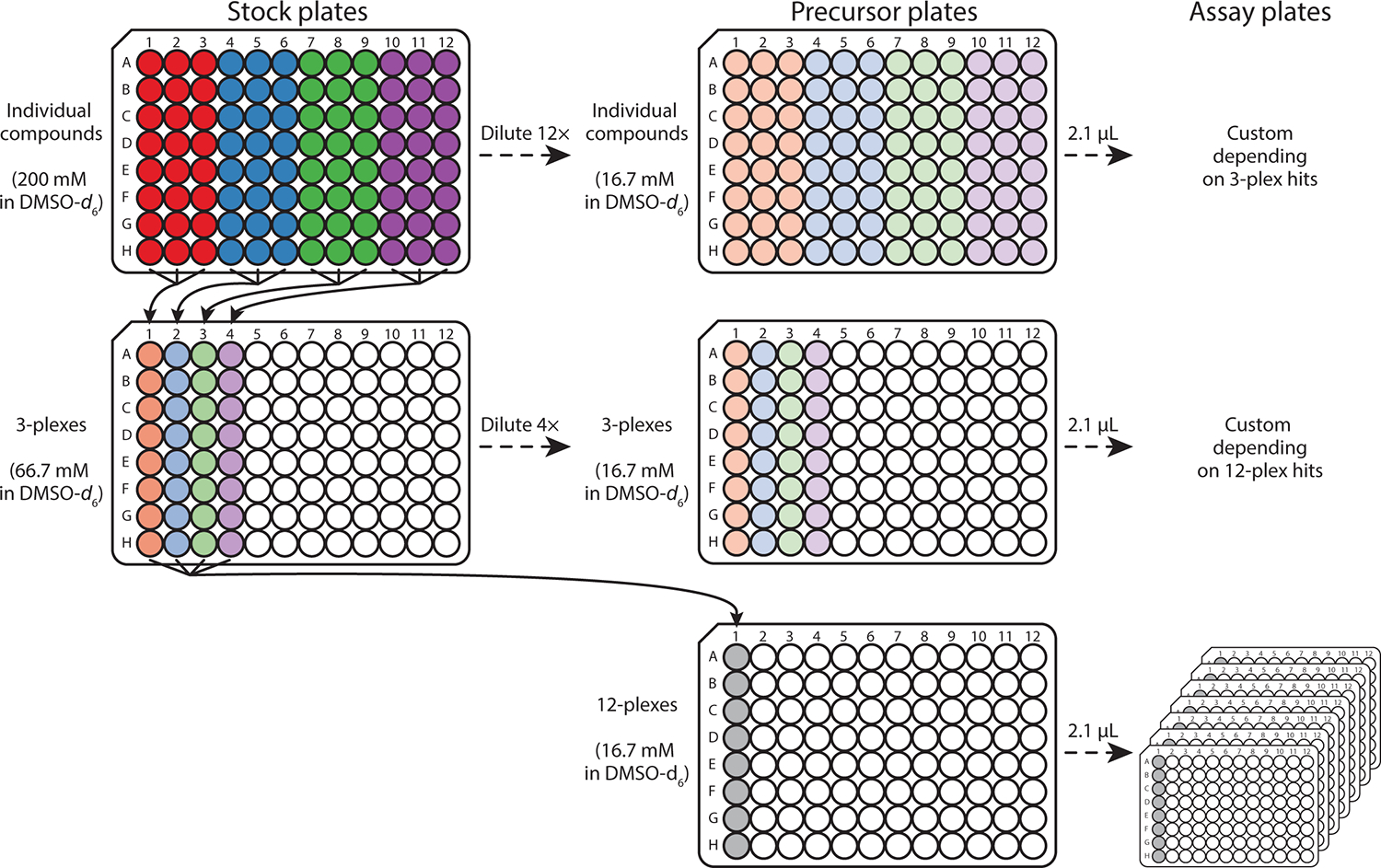
Schematic for multiplexing an example fragment library consisting of 96 individual compounds at 200 mM in DMSO-d₆ into 3- and 12-plex library samples. The individual compounds in the stock plate provided by the vendor are divided into four groups of three columns (red, blue, yellow, green) mixed into 3-plex samples containing 66.7 mM per compound. The four 3-plex samples from a transient stock plate (not stored long-term) are combined to create 12-plex samples in a precursor plate containing 16.7 mM per compound. Individual and 3-plex stock plates are diluted with DMSO-d₆ by 12- and 4-fold, respectively, to generate precursor plates (16.7 mM per compound). These precursor plates are then used to create assay plates to which protein is added for fragment screening.

Chemicals stored in DMSO at < 19 °C (the freezing point of DMSO) result in the library undergoing freeze-thaw cycles that can introduce atmospheric water into the wells over time and lead to fragment precipitation, hydrolysis, or other forms of degradation (Kozikowski et al., 2003). Initial and semiannual quality control of chemical fragments is necessary to ensure the purity and identity of the molecules over time (Keseru et al., 2016; Sreeramulu et al., 2020). Most molecules in our libraries have historically been stable for 2–4 years at 4 °C and longer at −80 °C.

3.1. Equipment

• Single- and multi-channel micropipettes (10, 200, and 1000 μL)

• Glass syringes (100–500 μL)

• 96-well v-bottomed plates (Greiner Bio-One #651201)

• Pierceable foil for 96-well plates (Sigma #A2350)

• Refrigerator

• Freezer

3.2. Reagents

• Fragment library

• DMSO-d₆

3.3. Library preparation

1. Obtain a chemical fragment library from a commercial/academic source or assemble a custom library. The individual compounds we purchased were shipped solubilized in DMSO-d₆ at 200 mM and stored in 96-well plates. Most vendors ensure that the purchased fragment library (a) follows the Ro3, (b) is PAINS-free, and (c) is soluble to 1 mM in H₂O and 200 mM in DMSO-d₆.

2. Store the ‘stock’ fragment library at −80 °C until further use.

3. Develop a labeling system for the fragments (individual and mixtures) in 96-well plates. Enter this information into a database for reference and label the 96-well plates accordingly. The 3D Shape Diverse library (Enamine), consisting of 1080 compounds shipped at 200 mM in DMSO-d₆, is used as an example for this procedure. This protocol has been optimized for fragment mixtures containing 3 and 12 compounds (3-plex and 12-plex, respectively). This library consists of two 12-plex (E1 and E2), five 3-plex (1–5), and fourteen individual (1–14) 96-well plates that are maintained in an Airtable (https://airtable.com/) database. Wells are labeled as follows:

   1. [E1/E2][coordinate in plate] for 12-plexes (e.g., E1A01)
   2. [E1/E2][coordinate in plate].[plate #][coordinate in plate] for 3-plexes (e.g., E1A01.01A02)
   3. [E1/E2][coordinate in plate].[plate #][coordinate in plate].[plate #][coordinate in plate] for individual samples (e.g., E1A01.01A02.01A02)

4. Create the individual compound ‘precursor’ plates by diluting the compounds from 200 to 16.7 mM in 1080 wells of 96-well v-bottom plates using DMSO-d₆ (Fig. 2). The resulting ‘precursor’ plates are stored at 4 °C until further use. A multichannel pipette (or robotics) is recommended to prepare the ‘precursor’ plates.

5. Generate 3-plex ‘stock’ matrixes by mixing 10 μL of three individual compounds at 200 mM each into 360 wells of 96-well v-bottom plates (Fig. 2). This ‘precursor’ plate is transient (not stored long-term) and immediately used for two purposes:

   1. Dilute the 3-plexes from 66.7 to 16.7 mM using DMSO-d₆ to generate 3-plex ‘precursor’ plates (Fig. 2).
   2. Prepare 12-plex ‘precursor’ matrixes by combining 10 μL of four 3-plexes containing 66.7 mM of each compound into 90 wells of a 96-well v-bottom plate. The 12-plexes will contain 16.7 mM of each compound (Fig. 2).

6. Transfer 2.1 μL from wells in 12-plex ‘precursor’ plates into ‘assay’ plates to prepare for the primary screen. The ‘assay’ plates are stored at 4 °C until used.

4. Primary screen

Creating fragment mixtures (e.g., 12-plexes and 3-plexes) for a series of sequential screens significantly reduces the number of samples and total experiment time compared to individually screening an entire library one molecule at a time. For example, individually screening a library of 1080 molecules requires 1080 samples and ~45 days of experiment time (~1 hr per ¹H–¹⁵N HSQC). Whereas 12-plex (90 samples; ~4 days), 3-plex (~44 samples; ~2 days), and individual (~33 samples; ~1 day) screening requires ~167 samples and ~7 days of total experiment time – assuming a 1% overall hit rate. Manually processing the many 2D NMR spectra from the screens is a laborious process that we have automated with Python scripts. The Python scripts: (a) expedite the data processing consistently for all spectra, (b) plot overlays and difference spectra to qualitatively compare the samples containing fragments to the DMSO-d₆-only control, and (c) quantify the changes in the spectra using difference intensity analysis (DIA) (Egner et al., 2018) and principal component analysis (PCA) using k-means clustering (Fig. 3).

Fig. 3.

¹H–¹⁵N HMQC spectra from a protein with 12-plexes (A) E1C03 and (B) E1A03 (red) overlayed on the control spectrum (without 12-plexes; black). The difference spectra for (C) E1C03 and (D) E1A03 highlight changes in the 12-plex spectra compared to the control spectrum. The peak intensities in the control spectrum are subtracted from the 12-plex spectra, and the resulting positive (blue) and negative (red) values appear on the difference spectra. (E) The spectra in a screen are differentiated by a variable number of k-means clusters (three for this example) using principal component analysis (PCA) generated by Python scripts. (F) The k-means clusters from panel E are then sorted by magnitude on a difference intensity analysis (DIA) plot with one (bold) and two (dashed) standard deviation lines. (A) E1C03 and (B) E1A03 were identified as a ‘hit’ and ‘non-hit’, respectively, for this protein based on the results from their (C/D) difference spectra, (E) PCA, and (F) DIA. The spectra and plots (A–F) are minimally formatted from the raw Python script output to illustrate the pipeline.

4.1. Equipment

• PAL liquid handling robot (LEAP Technologies) or similar robot capable of transferring liquid from 96-well plates into NMR tubes

• Single- and multi-channel micropipettes (10, 200, and 1000 μL)

• Glass syringes (100–500 μL)

• Reagent reservoir (Corning #4870)

• 1.7 mm NMR tubes in 96-tube rack format (Bruker #Z106462) or diameter tubes compatible with available NMR instrumentation

• NMR tube sealing balls (Bruker #Z72497)

• 96-well v-bottomed plates (Greiner Bio-One #651201)

• Pierceable foil for 96-well plates (Sigma #A2350)

• Centrifuge with deep well plate rack to spin down plates and deep well NMR tube rack

• 600 MHz Bruker Avance HD NMR spectrometer equipped with a 1.7 mm TCI Cryoprobe or similar NMR instrumentation

• SampleJet autosampler or similar NMR tube autosampler

4.2. Reagents

• Fragment library

• D₂O

• DMSO-d₆

• ¹⁵N-labeled protein

• NMR compatible buffer

4.3. 12-Plex NMR sample preparation

1. Remove one 96-well v-bottom 12-plex ‘assay’ plate from 4 °C and thaw. The plate will contain 2.1 μL of 16.67 mM of each compound in DMSO-d₆.

2. Add 2.1 μL of DMSO-d₆ to an empty well in the plate to make the control condition.

3. Resuspend protein in an appropriate buffer to the desired concentration. The default protein concentration for our screens ranges from 50 to 100 μM. Use a deuterated or phosphate buffer with 5–8% v/v D₂O and 0.02% w/v NaN₃.

4. Prepare 70 μL samples for the screen (plus one more for the DMSO-d₆ control) by adding 67.9 μL of protein solution to each well of the 96-well plate using a multichannel pipette. Place the tip of the pipette in the bottom of the well to mix the compound into the protein solution.

5. Seal the top of the 96-well plate with a foil seal. A foil seal prevents evaporation of the sample in the plate during filling, which can cause noticeable changes in the spectra as the robot takes hours to fill the NMR tubes.

6. Use the PAL liquid handling robot (or other means) to transfer 60 μL from the plate to a rack of 1.7 mm NMR tubes.

7. Centrifuge the NMR tube rack for 5 min at 500 × g to remove air bubbles and move the samples to the bottom of the tubes.

8. Seal the NMR tubes with sealing balls.

4.4. 12-Plex NMR data collection

1. Place the DMSO-d₆ control sample in the probe.

   1. Lock to D₂O.
   2. Tune ¹H and ¹⁵N, or nuclei appropriate for your experiment.
   3. Calculate the correct 90° proton pulse length (p1).
   4. Use these parameters for all experiments.

2. Open Iconnmr and queue all the experiments of each sample. Our standard scheme includes standard ¹H and T₂-filtered 1D experiments and ¹H–¹⁵N HSQC, SOFAST-HMQC, or NUS 2D experiments (determined in Section 2.5). We collect a 1D T₂-filtered NMR spectrum during a screen to monitor the stability of our fragment libraries over time.

3. Ensure each sample has its directory formatted appropriately.

   1. Proper formatting will be necessary for downstream data processing.
   2. The formatting consists of four fields, each separated by an underscore.
      [yyyymmdd]_[Protein name]_[Screen name]_[Compound/Plate/Well position]
   3. Below is an example of a directory name:
      20190503_CCL28_Maybridge-12plex_MA01

4. Queue the DMSO-d₆ control sample to run as the first and again as the last sample as a protein stability control.

4.5. 12-Plex NMR data processing

1. Gather data directories from all samples into a single directory.

2. Transfer the directory from the spectrometer to NMRbox (Maciejewski et al., 2017) for processing.

3. Transfer the processing directory with the required Python scripts to the top of the NMR data directory. Current processing directories can be downloaded from GitHub, https://github.com/mcwchembio/Fragment-Screen-Processing/tree/main/fragement_screen_processing_directory. Processing scripts rely on Python to automate the NMRPipe (Delaglio et al., 1995) data processing and analysis.

4. Navigate to the control directory using the command line and run the Bruker conversion script using the ‘bruker’ command.

5. Move the fid.com file to the fragment screening directory.

6. Generate a processing script called ‘nmr_ft.com’ to process the remaining 2D spectra.

7. Move the nmr_ft.com file to the processing directory.

8. Examine the #1_nmrpipe_process.py script:

   1. Line 15 should be changed to reflect the number of 2D spectra directories.
   2. Line 16 should be changed if a different name is used for the conversion script.
   3. Line 17 should be changed if a different name is used for the processing script.

9. Navigate back to the fragment screening directory and run #1_nmrpipe_process.py.

10. Run the #2_Interactive_2D_ppm_limits.py and use this to determine the optimal baseline contouring and X and Y limits for plotting data.

11. Run the #3_plotting_overlays_and_differences.py, follow the prompts, and use the baseline/limits parameters determined in Step 10. This will generate overlays and subtraction plots of the data (Fig. 3A–D).

12. Run the #4_DIA.py script following prompts with parameters determined in Step 10. This will generate a table with the difference intensities of each spectrum.

13. Run the #5_PCA.py script following prompts with parameters determined in Step 10. This will generate the principal components of each spectrum from the population of all spectra and plot the PCA plots (Fig. 3E).

14. Finally, run #6_kmeans.py. Choose the number of clusters just before the cumulative explained variance becomes linear. A plot will appear, and the user can accept or alter the number of clusters. This script runs k-means clustering from the principal components using the specified number of clusters to make DIA plots colored by the cluster (Fig. 3F).

15. Note the 12-plex samples to pursue for further screening to determine the individual compound(s) responsible for spectral changes. Then, screen the corresponding 3-plexes from the 12-plex hits and, subsequently, the individual molecules from the 3-plex hits.

4.6. 3-Plex and individual compound NMR screening

1. A new ‘assay’ plate is made for each 3-plex and individual screen by selecting the four 3-plex components of a 12-plex hit or the three individual fragments of a 3-plex hit (Fig. 2). Add 2.1 μL from the 3-plex or individual ‘precursor’ plate to a 96-well v-bottom ‘assay’ plate, similar to the 12-plex protocol in Section 4.3.

2. Then follow the 12-plex NMR sample prep in Section 4.3, starting with Step 2.

3. Data collection (Section 4.4) and analysis (Section 4.5) for 3-plex and individual screens are similar to the 12-plex protocol.

4.7. Hit detection from multiple data analysis products

Inspection of the overlays (plotted in png and pdf formats) will show any peak movements and loss/gain in intensities (Fig. 3A/C). Difference spectra (plotted in png and pdf formats) will highlight CSPs and better represent peak loss/gain as a couplet of positive and negative peaks (Fig. 3B/D). One can qualitatively determine which spectra are most like the control by inspecting the overlays and their respective difference spectra, then rule them out as nonbinders. Then, the data is quantitively analyzed using DIA and PCA with k-means clustering automatically with Python scripts.

4.8. Difference intensity analysis (DIA)

DIA calculates the total change in a spectrum collected from a sample with fragment(s) versus the DMSO-d₆ control spectrum without fragment(s) (Egner et al., 2018). Difference spectra are generated using the NMRadd function in NMRPipe to subtract the DMSO-d₆ control spectra from the small molecule-containing spectrum. Each point in the difference spectrum above or below the noise baseline, empirically determined for each screen, is then summed in aggregate. The sums will have a single positive and negative value for each spectrum. The values are visualized on DIA plots (plotted in png and pdf formats) to detect hits objectively (Fig. 3F). Fragment hits with real binding interactions typically have an equal positive and negative magnitude. DIA may miss small peak shifts, so overlays and difference plots may require manual inspection. Spectra are generally categorized by (a) little change (i.e., a non-binder) with a lack of significant positive and negative values, (b) clear CSP (i.e., a binder) with positive and negative values above and below one standard deviation and apparent peak shifts, or (c) global intensity loss (i.e., an aggregator) with mostly negative values and overall spectral loss.

4.9. Principal component analysis (PCA)

PCA is performed on the complete set of spectra in the screen, although regions outside the location of the peaks are removed before processing. Then, each 2D spectra is arrayed to a 1D data array and the Python package sklearn.Decomposition.PCA is implemented to compute the principal components (Fig. 3E). The principal components are visualized on PCA plots (plotted in png and pdf formats), which are ideal for discerning spectra labeled as binders, nonbinders, and global intensity loss. PCA can also separate distinct binding locations on the protein to inform future fragment linking or merging strategies to increase potency.

4.10. K-means clustering

In k-means clustering, a metric is added for all PCA dimensions in conjunction with the DIA values. The PCA usually generates approximately five new principal components with high explained variance. However, inspecting and visualizing five dimensions simultaneously is difficult. K-means clustering is used to bin spectra into a specified number of clusters across as many dimensions as indicated—the Python module sklearn.cluster. K-means is used for this purpose. A plot of the cumulative variance of the top principal components is displayed when this script is run. Typically, the number of clusters should equal the number of principal components before the cumulative variances become linear. The k-means clustering can be rerun multiple times to examine the differences in clustering with a different number of clusters selected.

4.11. NMRbox

While Python and NMRPipe are available for processing data locally on personal computers, the processing scripts on GitHub are written for NMRbox (Maciejewski et al., 2017). NMRbox maintains cloud-based Linux environments that provide a large software inventory and documentation to work with biomolecular NMR software. Academic, governmental, and non-profit accounts are free and easily created. Once an account is generated, the virtual machine is accessed through a VNC viewer or command line interface.

5. Hit validation and optimization

Once individual hits are identified, validation and binding affinity determination (e.g., K_d values) via NMR titration experiments and orthogonal biophysical techniques is critical, followed by chemical optimization via SAR studies. ¹H NMR spectra of the fragments identified as hits from the individual screen are verified before repurchasing compounds. Mass spectrometry can also be used to verify the identity of the molecules. Fragments from individual hits are repurchased from alternative sources if commercially available or synthesized from commercially available starting materials. Purchased and synthesized molecules are verified via ¹H NMR (and ¹³C NMR, X nuclei NMR, and mass spectrometry as appropriate) to ensure chemical identity with the fragment hit.

5.1. 2D NMR titrations

Each hit is titrated 0–6 mM (as solubility allows) against the ¹⁵N-labeled protein and monitored by the 2D NMR experiment used for the screen as determined in Section 2.2. Fragments that induce significant CSPs upon titration can be mapped using 2D NMR peak assignments onto known protein structures (if available) to reveal ligand-binding pockets (Zuiderweg, 2002). If not deposited at the Biological Magnetic Resonance Bank (BMRB) (Hoch et al., 2023) or otherwise available, sequence-specific resonance assignments are an additional nontrivial step needed to map CSPs to specific residues (Wuthrich, 1990). Global nonlinear fitting of the titration data from individual CSPs is performed to determine the binding affinity of the hits, which typically ranges from μM to low mM K_d values (Egner et al., 2018; Shishodia et al., 2022; Zhou et al., 2023).

5.2. Hit validation using orthogonal biophysical techniques

Although protein-detected NMR is less prone to artifacts as the entire protein is directly observed, orthogonal biophysical techniques are essential for hit validation. Orthogonal techniques include biolayer interferometry (BLI), surface plasmon resonance (SPR), microscale thermophoresis (MST), and isothermal titration calorimetry (ITC) (Campbell & Kim, 2007; Jerabek-Willemsen, Wienken, Braun, Baaske, & Duhr, 2011; Velázquez‐Campoy, Ohtaka, Nezami, Muzammil, & Freire, 2004; Wartchow et al., 2011). Ligand-observed NMR experiments, including water ligand observed via gradient spectroscopy (wLOGSY), STD, and Carr–Purcell–Meiboom–Gill (CPMG), can also be employed as orthogonal techniques for hit validation as reviewed in (Davis, 2021).

5.3. Structural activity relationships (SAR)

Optimization of hits via SAR studies is guided by binding affinity and residues involved in protein binding derived from the NMR experiments or other structural data. Systematic hit-to-lead generation is further enabled by the rising computational power of hardware and software, allowing fields such as cheminformatics (Wishart, 2007) and computational docking (Bender et al., 2021) to progress significantly. Coupling NMR data with computational docking, validated hits can be optimized into leads and further characterized by in vitro biophysical and biochemical assays. High-resolution structures of target protein bound to lead compounds can be solved by crystallography or other techniques, which can corroborate NMR data and computational docking and provide additional resolution of binding interactions to inform further computational docking studies. Finally, lead compounds can be assayed in cellular and in vivo model systems relevant to the protein target.

6. Expected Outcomes

Based on our experiences screening PBRM1 (Shishodia et al., 2022), CCL28 (Zhou et al., 2023), CXCL12, FIS1, and BRD4 (Egner et al., 2018), hit rates of 0.7–2% are expected with K_d values ranging from 45 μM to > 10 mM for the fragment hits. If the chemical shift assignments are known, then the chemical shift perturbations are expected to localize to discrete binding site(s) within the protein, which can be distinguished by discrete clusters in PCA plots.

7. Advantages

Small molecule ligands with high affinity and selectivity are essential tools for biomedical research and potentially valuable lead compounds for drug development. Chemical fragment screening is increasingly used to find molecules that bind a specific protein target. Protein-detected NMR provides several distinct advantages over other techniques for detecting weak interactions, validating candidate ligands, and identifying binding sites. The broader availability of commercial chemical fragment libraries and robots for NMR sample preparation and data acquisition permits fragment screening in more academic and industrial research environments than ever. The protocols and analytical methods described in this chapter were implemented and refined by scientists in the Program in Chemical Biology at the Medical College of Wisconsin over an eight-year period in which 16 different proteins were subjected to chemical fragment screening by 2D NMR.

8. Optimization and troubleshooting

Several screening campaigns encountered pitfalls that required careful planning or troubleshooting. As suggested in Section 3.3, a systematic naming and labeling scheme is essential to track compound location in 12-plex, 3-plex, and individual plates. As detailed in Section 4.3, covering 96-well plates with a pierceable foil seal was necessary to eliminate evaporation during sample mixing and dispensing into NMR tubes. Another lesson learned (or relearned) is the importance of ensuring the structural integrity of the target protein and chemical fragments. As demonstrated in the era of large-scale structural genomics projects (Jensen et al., 2010; Waltner, Peterson, Lytle, & Volkman, 2005), optimizing the expression construct is a critical early step in ensuring sufficient target protein stability over the weeks or months of a screening campaign. Target proteins that passed the one-week stability test may still degrade over the interval between multiplex screening cycles or while waiting for repurchased hits to arrive. While their usable lifetimes are typically longer than proteins, chemical fragment stocks can also degrade. Whether these problems are solved with improved storage conditions or by obtaining freshly purchased or purified material, NMR monitoring of native protein folding and structural integrity of fragments is necessary to avoid contamination of the data pipeline with misleading results. Ideally, the 1D and 2D spectra acquired during routine screening can longitudinally assess fragment and protein stability; however, periodic stability audits of the entire fragment library may also be warranted. Repurchasing compounds from a separate vendor also acts as a quality control step, as contaminants should be different while the main compounds should be the same. Heed nevertheless the ancient maxim ‘caveat emptor’, as chemical vendors achieve varying standards for quality control, documentation, and customer support.

9. Conclusion

In its current implementation, the Program in Chemical Biology fragment screening pipeline is available to Medical College of Wisconsin-affiliated investigators and external collaborators to launch small molecule discovery projects. This chapter is the first step in disseminating these tools to the scientific community. As appropriate, additional documentation and updates will be provided at GitHub, NMRBox, and other public repositories and resources.

10. Safety considerations

Nitrile or similar chemical-resistant gloves should be used when handling recombinant and biohazardous materials and hazardous chemicals. Chemical and biological waste should be disposed of through approved routes.

KEY RESOURCES TABLE.

REAGENT or RESOURCE	SOURCE	IDENTIFIER
Materials
Glass syringes (100 – 500 μL)	N/A	N/A
Micropipettes (10, 200, and 1000 μL)	N/A	N/A
Prometheus standard capillaries	Nanotemper	PR-C0002
1.7 mm NMR tubes	Bruker	Z106462
96-well v-bottomed plates	Greiner-Bio-One	651201
Pierceable foil for 96-well plates	Sigma	A2350
Reservoir trays	Corning	4870
NMR tube sealing balls	Bruker	Z72497
Equipment
NanoTemper Prometheus	Nanotemper	N/A
600 MHz NMR	Bruker	N/A
SampleJet autosampler	Bruker	N/A
Refrigerator/freezer	N/A	N/A
Centrifuge	N/A	N/A
Reagents
D2O	Cambridge Isotope Laboratories	DLM-4–50
DMSO-d6	Cambridge Isotope Laboratories	DLM-10–50
Fragment library	Enamine, Maybridge, Targetmol, Zenobia, etc.	N/A
Buffers
NMR compatible buffer	N/A	N/A
Proteins
15N-labeled protein	N/A	N/A
Software and Algorithms
NMRbox	https://nmrbox.nmrhub.org/	N/A
PAINS-remover	https://www.cbligand.org/PAINS/	N/A
Aggregator advisor	https://advisor.bkslab.org/	N/A

Abbreviations

BLI

biolayer interferometry

BMRB

Biological Magnetic Resonance Bank

CSP

chemical shift perturbation

CPMG

Carr–Purcell–Meiboom–Gill

DIA

difference intensity analysis

FBDD

fragment-based drug discovery

HBA

hydrogen bond acceptor

HBD

hydrogen bond donor

His₆

hexahistidine

HSQC

heteronuclear single quantum coherence

HMQC

heteronuclear multiple quantum coherence

ITC

isothermal titration calorimetry

MST

microscale thermophoresis

NMR

nuclear magnetic resonance

NRotB

number of rotatable bonds

NUS

non-uniform sampling

PAINs

pan-assay interference compounds

PCA

principal component analysis

Ro3

rule of 3

SAR

structural activity relationship

SPR

surface plasmon resonance

STD

saturation transfer difference

SUMO

small-ubiquitin-related modifier

wLOGSY

water ligand observed via gradient spectroscopy

cLogP

calculated log of the partition coefficient

References

- Baell JB, & Holloway GA (2010). New substructure filters for removal of pan assay interference compounds (PAINS) from screening libraries and for their exclusion in bioassays. Journal of Medicinal Chemistry, 53(7), 2719–2740. [DOI] [PubMed] [Google Scholar]
- Barna JCJ, Laue ED, Mayger MR, Skilling J, & Worrall SJP (1987). Exponential sampling, an alternative method for sampling in two-dimensional NMR experiments. Journal of Magnetic Resonance, 73, 69–77 (1969). [Google Scholar]
- Bender BJ, Gahbauer S, Luttens A, Lyu J, Webb CM, Stein RM, & Shoichet BK (2021). A practical guide to large-scale docking. Nature Protocols, 16(10), 4799–4832. [DOI] [PMC free article] [PubMed] [Google Scholar]
- Bieri M, Kwan AH, Mobli M, King GF, Mackay JP, & Gooley PR (2011). Macromolecular NMR spectroscopy for the non-spectroscopist: Beyond macro-molecular solution structure determination. The FEBS Journal, 278(5), 704–715. [DOI] [PubMed] [Google Scholar]
- Butt TR, Edavettal SC, Hall JP, & Mattern MR (2005). SUMO fusion technology for difficult-to-express proteins. Protein Expression and Purification, 43(1), 1–9. [DOI] [PMC free article] [PubMed] [Google Scholar]
- Campbell CT, & Kim G (2007). SPR microscopy and its applications to high-throughput analyses of biomolecular binding events and their kinetics. Biomaterials, 28(15), 2380–2392. [DOI] [PubMed] [Google Scholar]
- Congreve M, Carr R, Murray C, & Jhoti H (2003). A ‘rule of three’ for fragment-based lead discovery? Drug Discovery Today, 8(19), 876–877. [DOI] [PubMed] [Google Scholar]
- Davis BJ (2021). Fragment screening by NMR. Methods in Molecular Biology, 2263, 247–270. [DOI] [PubMed] [Google Scholar]
- Delaglio F, Grzesiek S, Vuister GW, Zhu G, Pfeifer J, & Bax A (1995). NMRPipe: A multidimensional spectral processing system based on UNIX pipes. Journal of Biomolecular NMR, 6(3), 277–293. [DOI] [PubMed] [Google Scholar]
- Delaglio F, Walker GS, Farley KA, Sharma R, Hoch JC, Arbogast LW, & Marino JP (2017). Non-uniform sampling for all: More NMR spectral quality, less measurement time. American Pharmaceutical Review, 20(4). [PMC free article] [PubMed] [Google Scholar]
- Egner JM, Jensen DR, Olp MD, Kennedy NW, Volkman BF, Peterson FC, & Hill RB (2018). Development and validation of 2D difference intensity analysis for chemical library screening by protein-detected NMR spectroscopy. Chembiochem: A European Journal of Chemical Biology, 19(5), 448–458. [DOI] [PMC free article] [PubMed] [Google Scholar]
- Erlanson DA (2014). Poll results: How do you store your fragment libraries?. Practical fragments. 3 March 2023. [Google Scholar]
- Erlanson DA, McDowell RS, & O’Brien T (2004). Fragment-based drug discovery. Journal of Medicinal Chemistry, 47(14), 3463–3482. [DOI] [PubMed] [Google Scholar]
- Fielding L (2003). NMR methods for the determination of protein-ligand dissociation constants. Current Topics in Medicinal Chemistry, 3(1), 39–53. [DOI] [PubMed] [Google Scholar]
- Fruh V, Zhou Y, Chen D, Loch C, Ab E, Grinkova YN, & Siegal G (2010). Application of fragment-based drug discovery to membrane proteins: Identification of ligands of the integral membrane enzyme DsbB. Chemistry & Biology, 17(8), 881–891. [DOI] [PMC free article] [PubMed] [Google Scholar]
- Ghosh S, Sengupta A, & Chandra K (2017). SOFAST-HMQC-An efficient tool for metabolomics. Analytical and Bioanalytical Chemistry, 409(29), 6731–6738. [DOI] [PubMed] [Google Scholar]
- Hoch JC, Baskaran K, Burr H, Chin J, Eghbalnia HR, Fujiwara T, & Yokochi M (2023). Biological magnetic resonance data bank. Nucleic Acids Research, 51(D1), D368–D376. [DOI] [PMC free article] [PubMed] [Google Scholar]
- Irwin JJ, Duan D, Torosyan H, Doak AK, Ziebart KT, Sterling T, & Shoichet BK (2015). An aggregation advisor for ligand discovery. Journal of Medicinal Chemistry, 58(17), 7076–7087. [DOI] [PMC free article] [PubMed] [Google Scholar]
- Jensen DR, Woytovich C, Li M, Duvnjak P, Cassidy MS, Frederick RO, & Volkman BF (2010). Rapid, robotic, small-scale protein production for NMR screening and structure determination. Protein Science, 19(3), 570–578. [DOI] [PMC free article] [PubMed] [Google Scholar]
- Jerabek-Willemsen M, Wienken CJ, Braun D, Baaske P, & Duhr S (2011). Molecular interaction studies using microscale thermophoresis. Assay and Drug Development Technologies, 9(4), 342–353. [DOI] [PMC free article] [PubMed] [Google Scholar]
- Keseru GM, Erlanson DA, Ferenczy GG, Hann MM, Murray CW, & Pickett SD (2016). Design principles for fragment libraries: Maximizing the value of learnings from pharma Fragment-Based Drug Discovery (FBDD) programs for use in academia. Journal of Medicinal Chemistry, 59(18), 8189–8206. [DOI] [PubMed] [Google Scholar]
- Kozikowski BA, Burt TM, Tirey DA, Williams LE, Kuzmak BR, Stanton DT, & Nelson SL (2003). The effect of freeze/thaw cycles on the stability of compounds in DMSO. Journal of Biomolecular Screening, 8(2), 210–215. [DOI] [PubMed] [Google Scholar]
- Kwan AH, Mobli M, Gooley PR, King GF, & Mackay JP (2011). Macromolecular NMR spectroscopy for the non-spectroscopist. The FEBS Journal, 278(5), 687–703. [DOI] [PubMed] [Google Scholar]
- Lichstein HC (1944). Studies of the effect of sodium azide on microbic growth and respiration: III. The effect of sodium azide on the gas metabolism of B. subtilis and P. aeruginosa and the influence of pyocyanine on the gas exchange of a pyocyanine-free strain of P. aeruginosa in the presence of sodium azide. Journal of Bacteriology, 47(3), 239–251. [DOI] [PMC free article] [PubMed] [Google Scholar]
- Maciejewski MW, Schuyler AD, Gryk MR, Moraru II, Romero PR, Ulrich EL, & Hoch JC (2017). NMRbox: A resource for biomolecular NMR computation. Biophysical Journal, 112(8), 1529–1534. [DOI] [PMC free article] [PubMed] [Google Scholar]
- McIntosh LP, & Dahlquist FW (1990). Biosynthetic incorporation of 15N and 13C for assignment and interpretation of nuclear magnetic resonance spectra of proteins. Quarterly Reviews of Biophysics, 23(1), 1–38. [DOI] [PubMed] [Google Scholar]
- Muchmore DC, McIntosh LP, Russell CB, Anderson DE, & Dahlquist FW (1989). Expression and nitrogen-15 labeling of proteins for proton and nitrogen-15 nuclear magnetic resonance. Methods in Enzymology, 177, 44–73. [DOI] [PubMed] [Google Scholar]
- Sheng C, & Zhang W (2013). Fragment informatics and computational fragment-based drug design: An overview and update. Medicinal Research Reviews, 33(3), 554–598. [DOI] [PubMed] [Google Scholar]
- Shishodia S, Nunez R, Strohmier BP, Bursch KL, Goetz CJ, Olp MD, & Smith BC (2022). Selective and cell-active PBRM1 bromodomain inhibitors discovered through NMR fragment screening. Journal of Medicinal Chemistry, 65(20), 13714–13735. [DOI] [PMC free article] [PubMed] [Google Scholar]
- Shuker SB, Hajduk PJ, Meadows RP, & Fesik SW (1996). Discovering high-affinity ligands for proteins: SAR by NMR. Science (New York, N. Y.), 274(5292), 1531–1534. [DOI] [PubMed] [Google Scholar]
- Sreeramulu S, Richter C, Kuehn T, Azzaoui K, Blommers MJJ, Del Conte R, & Schwalbe H (2020). NMR quality control of fragment libraries for screening. Journal of Biomolecular NMR, 74(10–11), 555–563. [DOI] [PMC free article] [PubMed] [Google Scholar]
- Taylor A, Doak BC, & Scanlon MJ (2018). Design of a fragment-screening library. Methods in Enzymology, 610, 97–115. [DOI] [PubMed] [Google Scholar]
- Tropea JE, Cherry S, & Waugh DS (2009). Expression and purification of soluble His (6)-tagged TEV protease. Methods in Molecular Biology, 498, 297–307. [DOI] [PubMed] [Google Scholar]
- Velázquez‐Campoy A, Ohtaka H, Nezami A, Muzammil S, & Freire E (2004). Isothermal titration calorimetry. Current Protocols in Cell Biology, 23(1) 17.18.1–17.18.24. [DOI] [PubMed] [Google Scholar]
- Waltner JK, Peterson FC, Lytle BL, & Volkman BF (2005). Structure of the B3 domain from Arabidopsis thaliana protein At1g16640. Protein Science, 14(9), 2478–2483. [DOI] [PMC free article] [PubMed] [Google Scholar]
- Wartchow CA, Podlaski F, Li S, Rowan K, Zhang X, Mark D, & Huang KS (2011). Biosensor-based small molecule fragment screening with biolayer interferometry. Journal of Computer-Aided Molecular Design, 25(7), 669–676. [DOI] [PubMed] [Google Scholar]
- Wishart DS (2007). Introduction to cheminformatics. Current Protocols in Bioinformatics, Chapter 14 Unit 14 11. [DOI] [PubMed] [Google Scholar]
- Wüthrich K (1986). Nuclear Magnetic Resonance of proteins and nucleic acids. Wiley. [Google Scholar]
- Wuthrich K (1990). Protein structure determination in solution by NMR spectroscopy. Journal of Biological Chemistry, 265(36), 22059–22062. [PubMed] [Google Scholar]
- Zhou AL, Jensen DR, Peterson FC, Thomas MA, Schlimgen RR, Dwinell MB, & Volkman BF (2023). Fragment-based drug discovery of small molecule ligands for the human chemokine CCL28. SLAS Discovery, 28, 163–169. [DOI] [PMC free article] [PubMed] [Google Scholar]
- Ziarek JJ, Peterson FC, Lytle BL, & Volkman BF (2011). Binding site identification and structure determination of protein-ligand complexes by NMR a semi-automated approach. Methods in Enzymology, 493, 241–275. [DOI] [PMC free article] [PubMed] [Google Scholar]
- Zuiderweg ER (2002). Mapping protein-protein interactions in solution by NMR spectroscopy. Biochemistry, 41(1), 1–7. [DOI] [PubMed] [Google Scholar]