Abstract
This article investigates the performance of three models - Autoregressive Integrated Moving Average (ARIMA), Threshold Autoregressive Moving Average (TARMA) and Evidential Neural Network for Regression (ENNReg) - in forecasting the Brent crude oil price, a crucial economic variable with a significant impact on the global economy. With the increasing complexity of the price dynamics due to geopolitical factors such as the Russo-Ukrainian war, we examine the impact of incorporating information on the war on the forecasting accuracy of these models. Our analysis shows that incorporating the impact of the war can significantly improve the forecasting accuracy of the models, and the ENNReg model with the inclusion of the dummy variable outperforms the other models during the war period. Including the war variable has enhanced the forecasting accuracy of the ENNReg model by 0.11%. These results carry significant implications regarding policymakers, investors, and researchers interested in developing accurate forecasting models in the presence of geopolitical events such as the Russo-Ukrainian war. The results can be used by the governments of oil-exporting countries for budget policies.
Keywords: Brent crude oil price, TARMA model, ENNReg model, ARIMA model, Russo-Ukrainian war, Forecasting, Nonlinear time series, Machine learning
1. Introduction
The Brent crude oil price is a crucial economic variable that has a significant impact on the global economy. The price dynamics of Brent crude oil have become increasingly complex in recent years, partly due to geopolitical factors such as the Russo-Ukrainian war [1,2]. The war has disrupted oil supplies and contributed to a heightened level of uncertainty in the oil market, making accurate forecasting of Brent crude oil prices challenging. Despite the abundance of literature on this subject, only a limited number of studies have successfully identified the significant change in the price of Brent crude oil resulting from the war. As a result, the effectiveness of existing models in predicting the price of Brent crude oil is likely to decrease when considering this structural break. Therefore, including the impact of the war when modeling the price of Brent can be beneficial for policymakers, especially in oil-producing nations, as it can aid them in designing appropriate budget policies.
In this article, we investigate the performance of three different models in forecasting the Brent crude oil price: the Autoregressive Integrated Moving Average (ARIMA) model [3], the Threshold Autoregressive Moving Average (TARMA) model [4,5], and the newly introduced Evidential Neural Network for Regression (ENNReg) model [[6], [7], [8]]. We also examine the impact of incorporating information on the Russo-Ukrainian war on the forecasting accuracy of these models.
The TARMA model is a nonlinear time series model that can capture the asymmetry of the price dynamics and the presence of different regimes in the data. The ENNReg model is a machine learning-based approach that can capture complex nonlinear relationships between the explanatory variables and the target variable. Finally, the ARIMA model is a widely used linear time series model that can capture the stochastic nature of the Brent crude oil price series. These models have the abilities to capture nonlinearity inherent in univariate time series such as Brent oil price.
Russo-Ukrainian on February 24, 2022, created significant uncertainty about the prices of fossil commodities such as oil. The eventual impacts of this war remain unknown [9,10]. It is important to study and estimate the effects of the Russian invasion on oil prices from the perspective of fossil commodities for some significant reasons. First, despite the war tending to be bilateral among Russia and Ukraine, it caused a considerable stir in the international community. In this context, Russo-Ukrainian War affects the global oil supply, which is the world's most used and traded commodity in the world [11,12]. However, this war has levied crippling sanctions such as expelling the Russian banks from SWIFT. These sanctions affected negatively on international trade among the world and Russia which supplies 19 % of the world's gas, and 13 % of global oil production.
Second, despite price oil prices declined significantly during the Coronavirus (COVID-19) pandemic crisis, there is a considerable increase in oil prices during the war, implying that this war has significant impacts on fossil commodities. There is a difference among this crisis (Russo-Ukrainian War) and prior crises in terms of the effect it has on the prices of oil. The significant impact of this war on the price oil implies that the economic effects of the Russo-Ukrainian war may be different from other recent crises such as COVID-19 [13].
The last political crises such as Russo-Ukrainian War led to an increase the uncertainty about the fossil commodities. This impact is still a burgeoning concern between the scholars. In this way [9], assessed the effects of Russian war on global financial markets, the authors demonstrate that the Russo-Ukrainian war adversely affects financial markets and this impact is not associated the level of the economy dependence on Russian oil [11]. confirm the Russo-Ukrainian war has a significant impact on the persistence and stability of the oil markets [14]. employed the Vector Autoregressive (VAR) [15,16] and examined the impact of Russian war on agricultural commodities and estimated their future performance. The findings suggested that Russian war has positive and significant impact on the agricultural commodities price [17]. examined the effect of the Russo-Ukrainian War on the commodity markets of oil, the threshold GARCH technique. The outcomes affirm the significant impact of the war on both in the natural gas and oil commodity markets.
While [18], used the GARCH model, and suggested that the reaction of the markets to the outbreak of the war is very limited pre and during the war. In the fact, an increase in oil price has a significant influence on the oil demand and supply. In this context [19], suggested that the Russo-Ukrainian War has led to a window of opportunity for new energy policies and strategies in the world centering on supporting renewable energy utilization and on the accelerated phase-out of oil energy utilization [11]. suggested that conflicts through Russo-Ukrainian led to significant fluctuations in fossil and other commodities prices.
Study [1] has created a novel application which can anticipate changes in crude oil prices by considering the effects of the COVID-19 pandemic and the Russia-Ukraine conflict. The researchers utilized a dataset spanning twenty-two years which included seven distinct features, such as crude oil opening and closing prices, as well as intraday highest and lowest values. They use machine learning and deep learning algorithms in conjunction with cross-validation to forecast crude oil prices. The outcomes of the study exhibited that the estimation performance was exceptional, with an average mean absolute error of more than 0.3786.
Study [20] explored the repercussions of geopolitical risk (GPR) on the volatility of stock returns in emerging markets, with a focus on China's CSI 300 index. The authors use GARCH-MIDAS model to analyse how GPR influences the Chinese stock market. They found that, aside from certain emerging economies, the majority of regional and global GPR had a significant impact on China's CSI index.
Study [21] investigates the relationship between food prices and macroeconomic factors, showing that both short- and long-term increases in energy prices lead to higher food prices. Moreover, a stronger US Dollar relative to the Iranian rial positively affects food prices in the long run. Another study uses panel spatial simultaneous equations models and GS2SLS method to explore the relationships between economic growth, carbon emissions, and renewable energy consumption in EU countries from 1995 to 2014. Positive spatial correlations exist between these variables across countries, with economic growth showing stronger correlation than CO2 emissions or renewable energy consumption. The study finds bidirectional links between economic growth and both carbon emissions and renewable energy consumption, while a unidirectional nexus exists between economic growth and renewable energy consumption [22]. Study [23] employs panel simultaneous equations models with a generalized method of moments estimator to investigate the relationships between ecological footprint, renewable energy consumption, and income in the G7 countries from 1990 to 2018. The results show a two-way association between gross domestic product and renewable energy, bidirectional links between EFP and outcome, and between EFP and renewable energy. Improving human capital has a positive and significant impact on income, environmental quality, and renewable energy consumption. Economic and social globalization does not significantly affect ecological footprint, while financial globalization has a negative and significant impact. Trade openness is positively and significantly connected with renewable energy consumption and income, potentially reducing environmental degradation [24,25].
Several methods have been employed to construct models for predicting the Brent oil price. These approaches comprise non-linear diffusion indices as proposed by Ref. [26], leveraging multilingual search engine data as presented in Refs. [27,28], using Bayesian Symbolic Regression as discussed by Ref. [29], utilizing Ivanov-Based LASSO Vector Autoregression as suggested by Ref. [30], incorporating a feed-forward neural network as suggested by Refs. [31,32], as well as employing Support Vector Machine as presented by Ref. [33], among others. Studies with comparable methods that consider geopolitical events in their analysis comprise [13,27,[34], [35], [36], [37]].
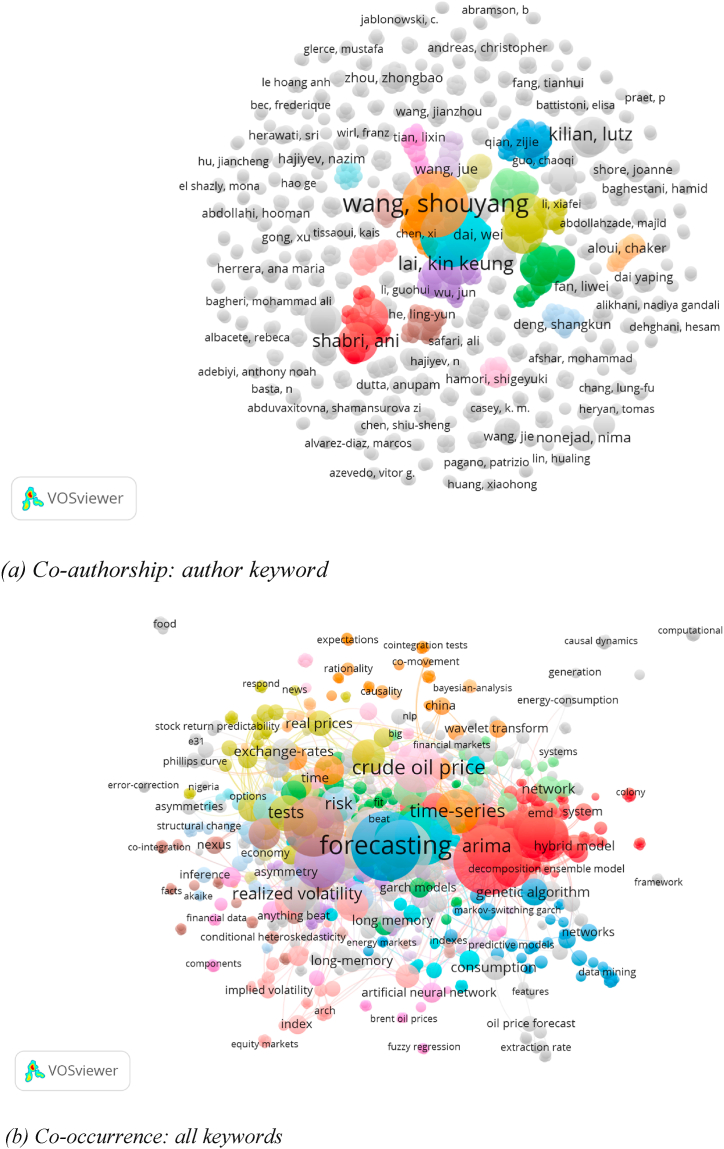
Fig. 1 summarises the literature on the Russio-Ukrainian war based on “Russia Ukraine war” keywords. Fig. 1 (a) is a summary of the contribution made by authors to the literature on the Russio-Ukrainian war. It shows that Wang's network has the largest contribution. Fig. 1 (b) presents the summary of co-occurrence based on all keywords. It shows that studies related to Brent oil price mainly focus on forecasting as it has the largest network.
Fig. 1.
Bibliometric analysis of the Russo-Ukraine war.
Our analysis shows that incorporating information on the Russo-Ukrainian war can significantly improve the forecasting accuracy of the models. In particular, the ENNReg model with the inclusion of the dummy variable outperforms the other models in forecasting the Brent crude oil price during the war period. Including the war variable has enhanced the forecasting accuracy of the ENNReg model by 0.11%. These results carry significant implications regarding policymakers, investors, and researchers who are interested in improving their understanding of the Brent crude oil price dynamics and developing accurate forecasting models in the presence of geopolitical events such as the Russo-Ukrainian war.
The current study makes a unique and significant contribution by being the first to employ an Evidential Neural Network based on Gaussian random fuzzy numbers (GRFNs) to predict Brent crude oil prices. Evidential Neural Networks are a recently developed machine learning technique that has shown promising results in various fields, including finance, engineering, and environmental studies [[6], [7], [8]]. This study's use of an Evidential Neural Network highlights the potential of this innovative approach for forecasting oil prices, which is a crucial area of research due to the significant impact of oil prices on the global economy.
By utilizing an evidential neural network, the study overcomes some of the limitations of traditional machine learning models, such as their inability to provide probabilistic predictions and handle uncertainty effectively. Evidential neural networks, on the other hand, offer a more robust approach that can model complex relationships between variables and provide quantified estimates of prediction uncertainty. This approach provides a more accurate representation of the data, allowing for more informed decision-making in various industries that rely on accurate oil price forecasts, such as energy, finance, and transportation.
The present study not only utilises the most recent methodology, but also takes into account the current Russo-Ukrainian conflict to evaluate how it affects the accuracy of the three models. To factor in the impact of this conflict, a dummy variable is integrated into the models with a value of 1 during the war period and 0 at other times.
The remaining components of the current work are divided into three parts: the methodology Section 2 the empirical results and discussion of findings are introduced in Section 3. The study's ramifications and policy framework are presented in Section 4.
2. Data and methodology
2.1. Data
The data set used for this research was acquired from the U.S Energy Information Administration's website (https://www.eia.gov/). Specifically, the Europe Brent spot price is utilized as the designated oil price for this study.
The BOP is normalised using the formula presented in Equation (1)
| (1) |
where is the original value of the series at time , is the minimum value of the BOP, is the maximum value of the BOP, and is the scaled value of the BOP at time .
2.2. ARIMA model
Studies [3] and [38] proposed the Autoregressive Integrated Moving Average (ARIMA) model, which is denoted by ARIMA (p,d,q) as shown in Equation (2). The three parameters p, d, and q respectively correspond to the autoregressive order, the order of integration, and the moving average order.
| (2) |
is the scaled BOP series assumed to be stationary, is the white noise error term, (the autoregressive term), (the moving average term) and is the backshift operator, otherwise known as lag operator expressed compactly as for . Similar studies that work with ARIMA include [[39], [40], [41]]. Therefore, the scaled BOP can be modelled as in Equation (3):
| (3) |
The new variable in Equation (3) stands for the dummy variable for period of Russian invasion of Ukraine. If the scaled BOP is nonstationary, then the most suitable model is ARIMA (, , ), otherwise ARMA (, ) will be right model.
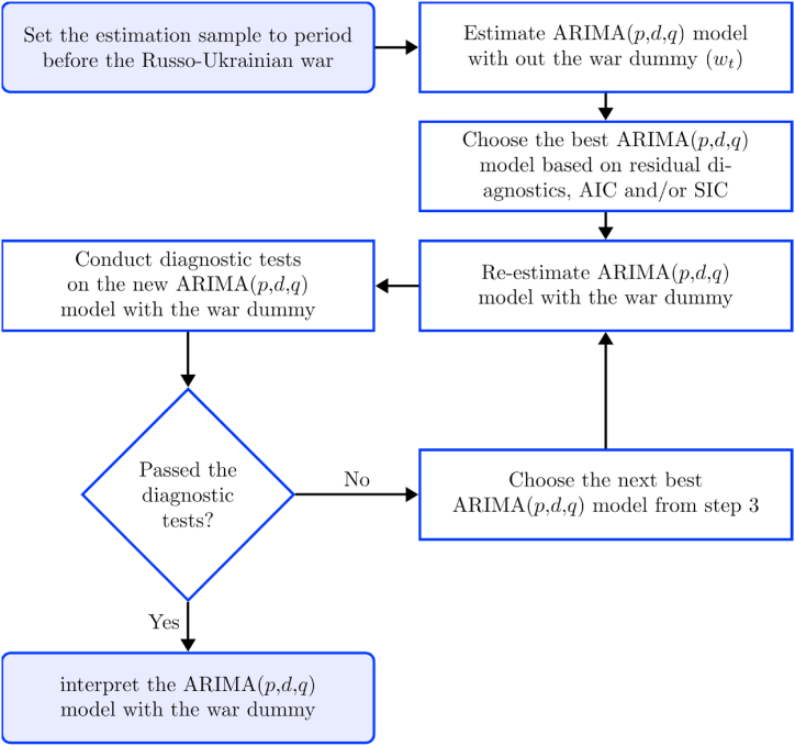
The steps are illustrated in Fig. 2 below.
Fig. 2.
Steps for the estimation of scaled BOP as an ARIMA (p,d,q) model.
2.3. TARMA model
Threshold Autoregressive Moving Average (TARMA) is a time series model that captures nonlinearity in the data by allowing the parameters of the autoregressive and moving average terms to vary depending on the level of the time series. The model is defined as follows:
where is the value of the scaled BOP at time , is the conditional mean of given past observations, is the error term at time , and are the coefficients of and , which, as in Equation (2), stand for the orders of the autoregressive and moving average terms respectively. The threshold parameter determines the switching point at which the model switches from a linear autoregressive moving average (ARMA) model to a simple random walk with drift.
The indicator function equals 1 if and 0 otherwise. This allows the model to capture the nonlinearity in the data by estimating different parameters for the ARMA model depending on the level of the time series. When the time series is below the threshold, the model reduces to a simple random walk with drift. When the time series is above the threshold, the model becomes an ARMA model.
The TARMA model can be estimated using maximum likelihood estimation or Bayesian methods. The estimation of the model requires specifying the orders and , the threshold , and the initial values for the parameters.
2.4. ENNReg model
The Evidential Neural Network (ENN) is a type of neural network that is capable of producing probabilistic predictions and uncertainty estimates. Unlike traditional neural networks that output point estimates, the ENN outputs a set of probability mass functions that represent the model's beliefs about the possible values of the target variable. These probability mass functions can be used to calculate various measures of uncertainty, such as confidence intervals and prediction intervals.
In the case of regression, the ENN takes as input a vector of predictor variables and produces a set of probability mass functions over the target variable . Each probability mass function corresponds to a different level of uncertainty, with the most certain distribution having the highest probability mass at a single value, and the most uncertain distribution having a uniform probability mass over a range of values. The ENN is trained by minimizing a loss function that measures the discrepancy between the predicted and actual probability mass functions.
Let be a vector of input features, and let be the target variable we wish to predict. The ENN model takes as input and outputs a set of probability mass functions over .
Let be the set of probability mass functions output by the ENN. Each element in represents the probability that takes on the value , given the input .
To train the ENN, we minimize a loss function that measures the discrepancy between the predicted and actual probability mass functions. One common choice of loss function is the Kullback-Leibler (KL) divergence, which is given by:
where is the number of possible values that can take on, and is the true probability mass function over (i.e., the actual distribution of in the training data) at value . The KL divergence measures the amount of information lost when approximating the true distribution with the predicted distribution.
During training, the weights of the ENN are adjusted using a standard backpropagation algorithm to minimize the loss function. Once the ENN has been trained, it can be used to make predictions on new inputs by outputting the set of probability mass functions . These probability mass functions can be used to calculate various measures of uncertainty, such as confidence intervals and prediction intervals.
2.5. Evaluation criteria
The evaluation of this study utilises several criteria, namely Mean Absolute Error (MAE), Root Mean Squared Error (RMSE), Mean Absolute Percentage Error (MAPE), Theil Inequality Coefficient (TIC) and Symmetric MAPE (SMAPE). These criteria are represented by equations 4, 5, 6, 7, 8, and 9 correspondingly.
| (4) |
| (5) |
| (6) |
| (7) |
| (8) |
| (9) |
Equations 4 to 9 use various symbols to represent the actual values of the scaled BOP , the forecast value of scaled BOP , the forecast length , and the training sample .
2.6. Model development
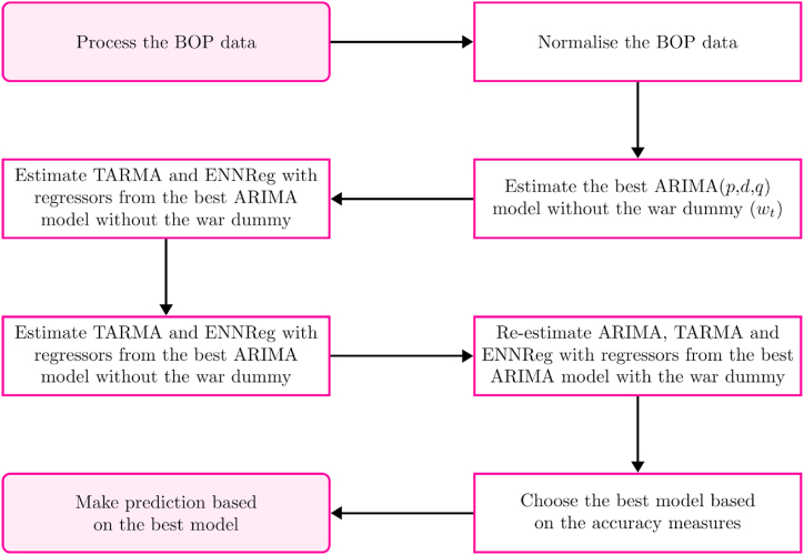
Fig. 3 illustrates the steps we follow to model the BOP based on ARIMA, TARMA and ENNReg.
Fig. 3.
Steps for modeling the BOP data.
2.7. The ARMA estimate
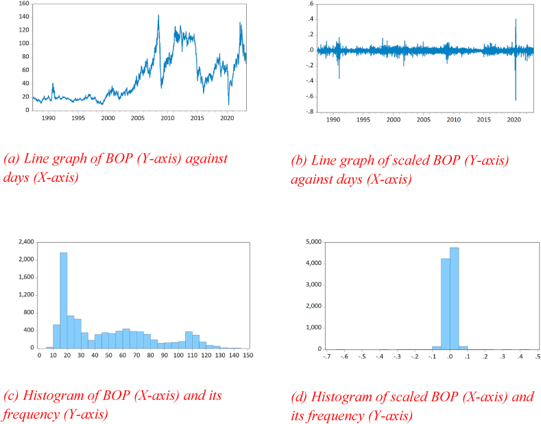
This paper focuses on examining the impact of the Russio-Ukrainian war on the forecast performance of Brent oil prices. To accomplish this, a new series {} is created by normalising the series of Brent oil price as described in Equation (1). The first step is to plot {} to determine if it is stationary. A quick review of Fig. 6 (b) indicates that the mean and variance are not constant. Moreover, formal unit root tests, such as the Augmented Dickey Fuller (ADF) test [42] and the Phillips-Perron (PP) test [43], demonstrate that the scaled BOP is not stationary at level. This indicates that the scaled Brent oil price () is I (1). Consequently, to model this nonstationary process, the scaled Brent oil price is represented as an ARMA (p,d,q) process.
Fig. 6.
Plots of BOP.
The war began around February 24, 2022, after the Ukraine invasion by the RF. We use the sample prior to the invasion because it is larger than the period after Russian invasion. Therefore, we begin by estimation of the ARIMA model for the scaled BOP ({}) series from 20th May 1987 to 23rd February 2022. The dummy representing the Russo-Ukrainian war () contains a series of zeros for period from 20th May 1987 to 23rd February 2022 and unity otherwise [15,16]. Specifically, for all February 24, 2022 and for all February 24, 2022. After obtaining the best ARIMA model for the scaled BOP, a new model is re-estimated which include the Russo-Ukrainian war dummy as described in [40] and [44].
In Fig. 7, the correlogram of the scaled BOP indicate the Autocorrelation Function (ACF) and Partial Autocorrelation Function (PACF), which are used to identify possible models. The significant lags in the PACF suggest the likely order of the autoregressive component (), while the significant lags in the ACF suggest the possible order of the moving average component (). Based on this analysis, potential models include ARIMA (1,1,0) AR (5,1,0), ARIMA (0,1,3), ARIMA (3,1,0), ARIMA (3,1,1), ARIMA (1,1,3), ARIMA (2,1,2), and others. All possible models are estimated and compared using measures such as residual diagnostics, , Akaike Information Criterion (AIC) and Schwarz Information Criterion (SIC). The value of the is used to determine the explanatory power of the regressors, and the SIC tends to choose a better model than the AIC in terms of parsimony.
Fig. 7.
Correlogram of the Brent oil price ().
Fig. 4 presents the ARMA criteria graph for the 20 best-performing ARIMA models according to their SIC values in ascending order [44]. Although ARIMA (0,1,1) has lower AIC value, the ARMA (1,1,0) model is selected to estimate the scaled BOP series since it has no redundant parameter estimates and autocorrelation. The series of scaled Brent oil price between 20th May 1987 and 25th June 2012 (training sample) was used to estimate the ARIMA (1,1,0) model. This was done using the maximum likelihood method with the OPG information matrix and the Marquardt step method.
Fig. 4.
The top 20 ARIMA models note; (X-axis) according to SIC (Y-axis).
2.8. Stability of the ARMA model
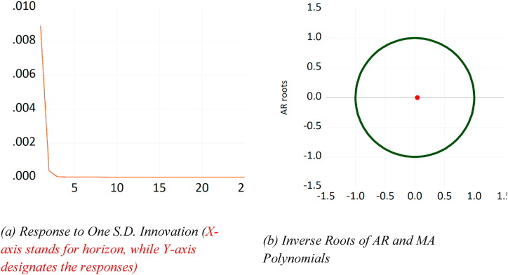
In Fig. 5 (a), we display the impulse response function (IRF) of the ARMA model we estimated. The graph in Fig. 5 (b) shows the roots of the AR and MA components. The IRF plot in Fig. 5 (a) indicates that the model is stable because the response decays after the initial shock. Similarly, the plot in Fig. 5 (b) indicates that the model is also stable because all inverted roots lie within the unit circle.
Fig. 5.
Graphs of impulse response and ARMA roots.
3. Results and discussions
The plots of the BOP series are depicted in Fig. 6. We begin by looking at the time series properties of the BOP. Fig. 6 (a) is the line graph of the Brent oil price at level, while Fig. 6 (b) is for the scaled Brent oil price. Fig. 6 (c) and 6 (d) represent the histograms of level and scaled Brent oil price respectively. Based on observations from Fig. 6 (a), it has been noted that the BOP does not exhibit a constant mean and variance. Consequently, formal unit root tests have been conducted to verify this, namely the Augmented Dickey Fuller (ADF) and Phillips-Perron (PP) tests, which were respectively developed by Refs. [42,43]. The results of these tests can be found in Table Table 1, and according to the ADF test, the BOP was found to be non-stationary at the level, but stationary at the first difference. This implies that the ADF unit root test has confirmed that the BOP follows an I (1) process.
Table 1.
Unit root tests for the scaled BOP.
| (a) ADF of the scaled BOP at level | |||||
|---|---|---|---|---|---|
| Variable | Deterministic Trend | Test Value | 5 % Critical Value | Prob | Decision |
| C | −1.664941 | −2.862371 | 0.4491 | I (1) | |
| C&T | −1.609926 | −3.411409 | 0.7892 | I (1) | |
| N | −0.753514 | −1.940937 | 0.3901 | I (1) | |
| (b) ADF C at first difference | |||||
|---|---|---|---|---|---|
| Variable | Deterministic Trend | Test Value | 5 % Critical Value | Prob | Decision |
| C | −50.46490 | −2.862371 | 1e-04 | I (1) | |
| C&T | −50.45899 | −3.411409 | 0e+00 | I (1) | |
| N | −50.47357 | −1.940937 | 1e-04 | I (1) | |
| (c) PP of the scaled BOP at level | |||||
|---|---|---|---|---|---|
| Variable | Deterministic Trend | Test Value | 5 % Critical Value | Prob | Decision |
| C | −1.653843 | −2.862371 | 0.4548 | I (1) | |
| C&T | −1.597656 | −3.411409 | 0.7941 | I (1) | |
| N | −0.748746 | −1.940937 | 0.3922 | I (1) | |
| (d) PP of the scaled BOP at first difference | |||||
|---|---|---|---|---|---|
| Variable | Deterministic Trend | Test Value | 5 % Critical Value | Prob | Decision |
| C | −50.40584 | −2.862371 | 1e-04 | I (1) | |
| C&T | −50.39976 | −3.411409 | 0e+00 | I (1) | |
| N | −50.41501 | −1.940937 | 1e-04 | I (1) | |
The performance of eight models was evaluated by estimating their forecasts. They include ARIMA selcected based on Schwarz Information Criteria (ARIMA-SIC), ARIMA based on Akaike Information Criterion (ARIMA-AIC), TARMA and ENNReg with variants of regressors as defined in Table 2. To determine the best model among the available options, various forecast statistics, presented in Equations 4 to 9, been computed for each model. These statistics are reported in Tables Table 3 and Table 4. The model with the minimum value for these forecast statistics is considered the best choice. The TARMA model with war dummy is not reported as its forecast performance is not better than that of the TARMA model.
Table 2.
Definition of models.
| Model | Order | Definition |
|---|---|---|
| ARIMA-SIC | ar [0,1,1] | ARIMA based on SIC |
| ARIMA–SIC–WAR | ar [0,1,1] | ARIMA based on SIC with war dummy |
| ARIMA-AIC | ar [1,1,2] | ARIMA based on AIC |
| ARIMA-AIC-WAR | ar [1,1,2] | ARIMA based on AIC with war dummy |
| TARMA | TARMA (1,1,2,1) | TARMA without war dummy |
| TARMA-WAR | TARMA (1,1,2,1) | TARMA with war dummy |
| ENNREG | – | ENNREG without war dummy |
| ENNREG-WAR | – | ENNREG with war dummy |
Table 3.
Results of the BOP forecast evaluation for the training sample.
| Model | RMSE | MAE | SMAPE | Theil U1 |
|---|---|---|---|---|
| ARIMA-SIC | 0.007439 | 0.004445 | 3.001417 | 0.011824 |
| ARIMA–SIC–WAR | 0.007439 | 0.004445 | 3.000966 | 0.011823 |
| ARIMA-AIC | 0.007440 | 0.004448 | 2.999182 | 0.011825 |
| ARIMA-AIC-WAR | 0.007440 | 0.004448 | 2.998591 | 0.011825 |
| TARMA | 0.007430 | 0.004443 | 2.998044 | 0.011813 |
| ENNREG | 0.007422 | 0.004453 | 3.075503 | 0.011804 |
| ENNREG-WAR | 0.007426 | 0.004451 | 3.008297 | 0.011807 |
Table 4.
Results of the BOP forecast for the testing sample.
| Model | RMSE | MAE | SMAPE | Theil U1 |
|---|---|---|---|---|
| ARIMA-SIC | 0.011460 | 0.007823 | 2.125137 | 0.011272 |
| ARIMA–SIC–WAR | 0.011458 | 0.007825 | 2.125269 | 0.011271 |
| ARIMA-AIC | 0.011453 | 0.007818 | 2.122844 | 0.011265 |
| ARIMA-AIC-WAR | 0.011451 | 0.007820 | 2.122960 | 0.011264 |
| TARMA | 0.011455 | 0.007814 | 2.122288 | 0.011269 |
| ENNREG | 0.011435 | 0.007826 | 2.108600 | 0.011248 |
| ENNREG-WAR | 0.011423 | 0.007810 | 2.120558 | 0.011237 |
We begin by determining the best ARIMA models based on SIC and AIC values. We then use the lagged values of the BOP and war dummy as the regressors for other models. The sample has been split into two separate subsets: a training sub-sample, which comprises 70 % of the total data, and a testing sub-sample, which makes up 30 % of the data.
According to several authors including [41,45], and [40], the scaled BOP can be expressed as an ARIMA (p, 1,q) process because it is integrated of order one. To determine the optimal values for p and q, the combination that results in the lowest SIC with white-noise errors is chosen.
To ascertain the potential moving average order, the ACF is employed. Conversely, the PACF is used to determine the possible autoregressive order. The ACF and PACF graphs are depicted in Fig. 7 (a) and 7 (b) respectively.
Table 3 displays the performance of the top models used to forecast the BOP for the training sample. The table outlines the forecast statistics for the most successful models used to forecast the BOP for the training sample. Based on the RMSE and Theil measures, the ENNReg model emerges as the best-performing model. This is evident from the results presented in the table. However, based on MAE and SMAPE, the TARMA model is the best. As the training sample does not cover the war period, we can observe that incorporating the war dummy has no impact on the models’ predictive capacity.
Table 4 presents the forecast assessment for the testing sample, which includes the forecast statistics for the top-performing models for the BOP. According to the table, ENNReg-WAR outperforms other models based on RMSE, MAE, and Theil , followed by ENNReg based on SMAPE and Theil , and then ARIMA-AIC-WAR based on MAPE. It is crucial to note that when other accuracy measures conflict with RMSE, the RMSE measure takes precedence.
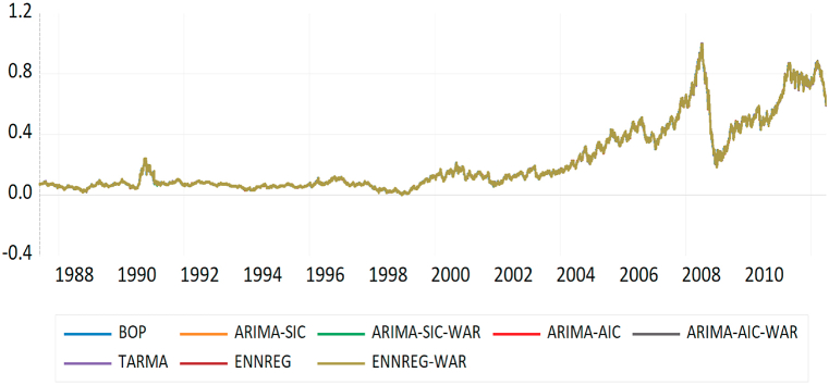
Fig. 8, Fig. 9 are used to compare the predicted values of the scaled BOP for the training and testing samples respectively. The line graphs for the actual and predicted values of the BOP are almost identical, indicating the effectiveness of ARIMA, TARMA, and ENNReg in forecasting the scaled BOP.
Fig. 8.
Forecast performance for the training sample (source: authors).
Fig. 9.
Forecast performance for the testing sample (source: authors).
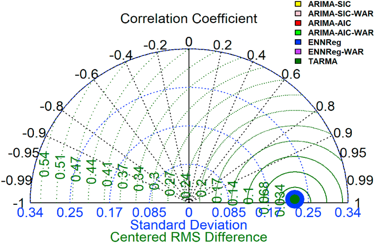
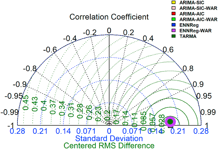
Fig. 10 is the taylor diagram for the training sample, while Fig. 11 is for the testing sample. The size of the dots represents the predictive accuracy of the models in terms of RMSE, with the largest dot indicating the best performing model. The diagram in Fig. 10 shows that ENNReg has the highest accuracy in forecasting the BOP for the training sample. Meanwhile, the diagram in Fig. 11 indicates that ENNReg-WAR outperforms other models in terms of forecasting accuracy for the testing sample. These figures provide a visual summary of Table 3, Table 4, respectively.
Fig. 10.
Taylor diagram comparing the models' performance for the training sample.
Fig. 11.
Taylor diagram comparing the models' performance for the testing sample.
Fig. 12, Fig. 13 depict the fan plots for the training and testing samples, respectively, which showcase the performance of seven models based on their RMSE. A model with a smaller sector angle in the fan plot indicates a better predictive performance. These two figures are in agreement with the findings presented in Fig. 10, Fig. 11.
Fig. 12.
Fan plot according to the RMSE for the training sample.
Fig. 13.
Fan plot according to the RMSE for the testing sample.
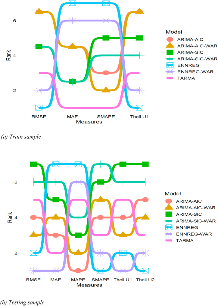
Fig. 14 (a) and 14 (b) depict the summarize the accuracy measures for the training and testing samples respectively. The figures show the rank of each model along the Y axis. It conforms with the information provided in Table 3, Table 4, as it shows that ENNReg-WAR is the best performing model.
Fig. 14.
Bump chart of the accuracy measures.
After evaluating the predictive performance of the seven best-performing models presented in this study, it can be observed that ENNReg-WAR and ENNReg are the most effective models. The superior performance of the ENNReg model can be attributed to its ability to incorporate nonlinearity in parameter estimates, as suggested by Ref. [27]. Furthermore, including the war dummy in the estimated models produces better predictive accuracy than using individual models without the war dummy.
The performance of the ENNReg model in this study, which incorporates information on the Russo-Ukrainian war, outperforms the other models in forecasting Brent crude oil prices during the war period. This finding is consistent with previous studies that have shown the importance of incorporating geopolitical events in forecasting crude oil prices. This is in line with the results of [27,[34], [35], [36], [37]]. For example, a study by Ref. [27] found that a VAR model that incorporates information on geopolitical events such as the US-Iran tensions and the COVID-19 pandemic outperformed other models in forecasting crude oil prices. Similarly, a study by Ref. [37] found that incorporating information on the COVID-19 pandemic and geopolitical events such as the US-China trade war improved the accuracy of forecasting models for crude oil prices.
However, it is important to note that the performance of the ENNReg model may vary depending on the time period and the specific geopolitical event being incorporated. For example, studies by Ref. [46] found that a hybrid model that combines wavelet decomposition and neural network models outperformed other models in forecasting crude oil prices during the COVID-19 pandemic but did not perform as well during the 2014 oil price drop.
The study focused on how the Russo-Ukrainian war affected forecasting accuracy in the estimated models. The study does not consider other geopolitical events, like conflicts in the Middle East and oil-producing country sanctions. Additionally, the study does not incorporate other scenarios, such as news sentiment and climatic changes, that can lead to structural break in the BOP. Incorporating news sentiment data into forecasting models could also be explored to understand its influence on oil prices.
Overall, these findings suggest that while incorporating information on geopolitical events can improve the accuracy of forecasting models for crude oil prices, the specific model and approach used may vary depending on the time period and the nature of the event being incorporated. Therefore, it is important for researchers to continue to explore and develop new approaches for incorporating information on geopolitical events in forecasting crude oil prices.
4. Conclusion
In conclusion, this study provides valuable insights into the performance of three popular models - TARMA, ENNReg, and ARIMA - in forecasting the Brent crude oil price, a crucial economic variable with a significant impact on the global economy. By examining the impact of incorporating information on the Russo-Ukrainian war, we find that the inclusion of the dummy variable and geopolitical risk indices can significantly improve the forecasting accuracy of the models. Notably, the ENNReg model outperforms the other models during the war period, highlighting the importance of considering geopolitical events when developing forecasting models. These results carry significant implications regarding policymakers, investors, and researchers interested in accurately forecasting the Brent crude oil price in the presence of geopolitical events. Overall, this study underscores the importance of continuously evaluating and improving forecasting models to provide valuable insights into complex economic dynamics.
The primary finding of our analysis is that the Russo-Ukrainian war caused a structural break in the BOP, resulting in reduced effectiveness of existing forecasting models. However, when we integrated the impact of the war into the analysis, all three models showed improved forecast accuracy. This highlights the importance of considering geopolitical events when modeling time series variables to gain better insights and make more informed policy recommendations.
The current study focused on the impact of the Russo-Ukrainian war on the forecasting accuracy of the models. A future study could examine the impact of other geopolitical events, such as conflicts in the Middle East and sanctions on oil-producing countries, on the forecasting accuracy of the models. Other forecasting models can be used to predict Brent crude oil prices. A future study could compare the performance of these models with TARMA, ENNReg, and ARIMA. News sentiment can impact the Brent crude oil prices as it can influence the demand and supply of oil. A future study could incorporate news sentiment data into the forecasting models to examine its impact on the forecasting accuracy. A future study could examine the impact of climate change on the forecasting accuracy of the models. A future study could compare the performance of the models for different time periods to examine their robustness.
Data availability statement
The data that support the findings of this study are openly available in U.S. Energy Information Administration at https://www.eia.gov/dnav/pet/hist/RBRTED.htm.
Funding
The authors received no funding for this study.
Additional information
No additional information is available for this paper.
CRediT authorship contribution statement
Sagiru Mati: Conceptualization, Formal analysis, Methodology, Software, Writing – original draft. Magdalena Radulescu: Project administration, Supervision, Validation, Writing – original draft. Najia Saqib: Investigation, Methodology, Writing – review & editing. Ahmed Samour: Investigation, Writing – review & editing. Goran Yousif Ismael: Data curation, Funding acquisition, Writing – review & editing. Nazifi Aliyu: Methodology, Validation, Writing – review & editing.
Declaration of competing interest
The authors declare that they have no known competing financial interests or personal relationships that could have appeared to influence the work reported in this paper.
Acknowledgments
The third author would like to thank Prince Sultan University for their support.
Contributor Information
Sagiru Mati, Email: sagirumati@gmail.com.
Magdalena Radulescu, Email: magdalena.radulescu@upit.ro.
Najia Saqib, Email: nsaqib@psu.edu.sa.
Ahmed Samour, Email: asamour@du.edu.om.
Goran Yousif Ismael, Email: goran.yousif@noble.edu.krd.
Nazifi Aliyu, Email: Nazifi.aliyu@yahoo.com.
References
- 1.Jahanshahi H., Uzun S., Kacar S., Yao Q., Alassafi M.O. Artificial intelligence-based prediction of crude oil prices using multiple features under the effect of Russia-ukraine war and COVID-19 pandemic. Mathematics. 2022;10 doi: 10.3390/math10224361. [DOI] [Google Scholar]
- 2.Wang X., Li X., Li S. Point and interval forecasting system for crude oil price based on complete ensemble extreme-point symmetric mode decomposition with adaptive noise and intelligent optimization algorithm. Appl. Energy. 2022;328 doi: 10.1016/j.apenergy.2022.120194. [DOI] [Google Scholar]
- 3.Box G.E., Jenkins G.M. Holden-Day; 1976. Time Series Analysis: Forecasting and control san francisco, Calif. [Google Scholar]
- 4.Tong H. 1978. On a Threshold Model. [Google Scholar]
- 5.Tong H. Threshold models in time series analysissome reflections. J. Econom. 2015;189:485–491. doi: 10.1016/j.jeconom.2015.03.039. [DOI] [Google Scholar]
- 6.Denœux T. Belief Functions: Theory and Applications. Springer International Publishing; 2022. An evidential neural network model for regression based on random fuzzy numbers; pp. 57–66. [DOI] [Google Scholar]
- 7.Denœux T. Reasoning with fuzzy and uncertain evidence using epistemic random fuzzy sets: general framework and practical models. Fuzzy Set Syst. 2023;453:1–36. doi: 10.1016/j.fss.2022.06.004. [DOI] [Google Scholar]
- 8.Denoeux T. 2023. Quantifying Prediction Uncertainty in Regression Using Random Fuzzy Sets: the ENNreg Model. [DOI] [Google Scholar]
- 9.Lo G.-D., Marcelin I., Bassène T., Sène B. The russo-Ukrainian war and financial markets: the role of dependence on Russian commodities. Finance Res. Lett. 2022;50 doi: 10.1016/j.frl.2022.103194. [DOI] [Google Scholar]
- 10.Pata U.K., Samour A. Do renewable and nuclear energy enhance environmental quality in France? A new EKC approach with the load capacity factor. Prog. Nucl. Energy. 2022;149 doi: 10.1016/j.pnucene.2022.104249. [DOI] [Google Scholar]
- 11.Adekoya O.B., Asl M.G., Oliyide J.A., Izadi P. Multifractality and cross-correlation between the crude oil and the european and non-european stock markets during the Russia-ukraine war. Resour. Pol. 2023;80 doi: 10.1016/j.resourpol.2022.103134. [DOI] [Google Scholar]
- 12.Kartal M.T., Samour A., Adebayo T.S., Depren S.K. Do nuclear energy and renewable energy surge environmental quality in the United States? New insights from novel bootstrap fourier granger causality in quantiles approach. Prog. Nucl. Energy. 2023;155 doi: 10.1016/j.pnucene.2022.104509. [DOI] [Google Scholar]
- 13.Ha L.T. A wavelet analysis of dynamic connectedness between geopolitical risk and renewable energy volatility during the COVID-19 pandemic and Ukraine-russia conflicts. Environ. Sci. Pollut. Control Ser. 2023 doi: 10.1007/s11356-023-26033-1. [DOI] [PMC free article] [PubMed] [Google Scholar]
- 14.Aliu F., Hašková S., Bajra U.Q. Consequences of Russian invasion on Ukraine: evidence from foreign exchange rates. J. Risk Finance. 2023;24:40–58. doi: 10.1108/JRF-05-2022-0127. [DOI] [Google Scholar]
- 15.Mati S., Civcir I., Özdeşer H. ECOWAS common currency, a mirage or possibility? Panoeconomicus. 2023;70:239–260. doi: 10.2298/pan191119015m. [DOI] [Google Scholar]
- 16.Mati S., Civcir I., Ozdeser H. ECOWAS common currency: how prepared are its members? Invest. Economica. 2019;78:89–119. doi: 10.22201/fe.01851667p.2019.308.69625. [DOI] [Google Scholar]
- 17.Vasileiou E. Abnormal returns and anti-leverage effect in the time of Russo-Ukrainian War 2022: evidence from oil, wheat and natural gas markets. J. Econ. Stud. 2023;50(5):1063–1072. doi: 10.1108/JES-04-2022-0235. [DOI] [Google Scholar]
- 18.Fiszeder P., Małecka M. Forecasting volatility during the outbreak of Russian invasion of Ukraine: application to commodities, stock indices, currencies, and cryptocurrencies, Equilibrium. Quarterly Journal of Economics and Economic Policy. 2022;17:939–967. doi: 10.24136/eq.2022.032. [DOI] [Google Scholar]
- 19.Steffen B., Patt A. A historical turning point? Early evidence on how the Russia-ukraine war changes public support for clean energy policies. Energy Res. Social Sci. 2022;91 doi: 10.1016/j.erss.2022.102758. [DOI] [Google Scholar]
- 20.Yang M., Zhang Q., Yi A., Peng P. Geopolitical risk and stock market volatility in emerging economies: evidence from GARCH-MIDAS model. Discrete Dynam Nat. Soc. 2021:2021. doi: 10.1155/2021/1159358. [DOI] [Google Scholar]
- 21.Radmehr R., Henneberry S.R. Energy price policies and food prices: empirical evidence from Iran. Energies. 2020;13:4031. doi: 10.3390/en13154031. [DOI] [Google Scholar]
- 22.Radmehr R., Henneberry S.R., Shayanmehr S. Renewable energy consumption, CO2 emissions, and economic growth nexus: a simultaneity spatial modeling analysis of EU countries. Struct. Change Econ. Dynam. 2021;57:13–27. doi: 10.1016/j.strueco.2021.01.006. [DOI] [Google Scholar]
- 23.Radmehr R., Shayanmehr S., Ali E.B., Ofori E.K., Jasińska E., Jasiński M. Exploring the nexus of renewable energy, ecological footprint, and economic growth through globalization and human capital in G7 economics. Sustainability. 2022;14 doi: 10.3390/su141912227. [DOI] [Google Scholar]
- 24.Pata U.K., Samour A. Assessing the role of the insurance market and renewable energy in the load capacity factor of OECD countries. Environ. Sci. Pollut. Control Ser. 2023;30:48604–48616. doi: 10.1007/s11356-023-25747-6. [DOI] [PubMed] [Google Scholar]
- 25.Jahanger A., Balsalobre-Lorente D., Ali M., Samour A., Abbas S., Tursoy T., Joof F. vol. 0. Energy & Environment; 2023. (Going Away or Going Green in ASEAN Countries: Testing the Impact of Green Financing and Energy on Environmental Sustainability). [DOI] [Google Scholar]
- 26.Zhang Y., He M., Wen D., Wang Y. Forecasting crude oil price returns: can nonlinearity help? Energy. 2023;262 doi: 10.1016/j.energy.2022.125589. [DOI] [Google Scholar]
- 27.Li J., Tang L., Wang S. Forecasting crude oil price with multilingual search engine data. Phys. Stat. Mech. Appl. 2020:551. doi: 10.1016/j.physa.2020.124178. [DOI] [Google Scholar]
- 28.Li S., Samour A., Irfan M., Ali M. Role of renewable energy and fiscal policy on trade adjusted carbon emissions: evaluating the role of environmental policy stringency. Renew. Energy. 2023;205:156–165. doi: 10.1016/j.renene.2023.01.047. [DOI] [Google Scholar]
- 29.Drachal K. Forecasting the crude oil spot price with bayesian symbolic regression. Energies. 2023;16 doi: 10.3390/en16010004. [DOI] [Google Scholar]
- 30.Ding Y., He D., Wu J., Xu X. Crude oil spot price forecasting using ivanov-based LASSO vector autoregression. Complexity. 2022:2022. doi: 10.1155/2022/5011174. [DOI] [Google Scholar]
- 31.Kariyam K., Yuwinda F.A.P. In: 2ND INTERNATIONAL CONFERENCE ON CHEMISTRY, CHEMICAL PROCESS AND ENGINEERING (IC3PE) Fatimah I., Kawasaki H., Kamari A., Chuenchom L., Kurniawan S., Sahroni I., Musawwa M., editors. Univ Islam Indonesia, Chem Dept; Indonesian Chem Soc; 2018. Comparison study of crude oil price forecasting using generalized regression neural network and feed forward neural network. [DOI] [Google Scholar]
- 32.Fang T., Zheng C., Wang D. Forecasting the crude oil prices with an EMD-ISBM-FNN model. Energy. 2023;263 doi: 10.1016/j.energy.2022.125407. [DOI] [Google Scholar]
- 33.Yu L., Zhang X., Wang S. Assessing potentiality of support vector machine method in crude oil price forecasting. Eurasia J. Math. Sci. Technol. Educ. 2017;13:7893–7904. doi: 10.12973/ejmste/77926. [DOI] [Google Scholar]
- 34.Miao H., Ramchander S., Wang T., Yang D. Influential factors in crude oil price forecasting. Energy Econ. 2017;68:77–88. doi: 10.1016/j.eneco.2017.09.010. [DOI] [Google Scholar]
- 35.Nonejad N. Forecasting crude oil price volatility out-of-sample using news-based geopolitical risk index: what forms of nonlinearity help improve forecast accuracy the most? Finance Res. Lett. 2022;46 doi: 10.1016/j.frl.2021.102310. [DOI] [Google Scholar]
- 36.Zhang H.-L., Liu C.-X., Zhao M.-Z., Sun Y. Economics, fundamentals, technology, finance, speculation and geopolitics of crude oil prices: an econometric analysis and forecast based on data from 1990 to 2017. Petrol. Sci. 2018;15:432–450. doi: 10.1007/s12182-018-0228-z. [DOI] [Google Scholar]
- 37.Alam M.S., Murshed M., Manigandan P., Pachiyappan D., Abduvaxitovna S.Z. Forecasting oil, coal, and natural gas prices in the pre-and post-COVID scenarios: contextual evidence from India using time series forecasting tools. Resour. Pol. 2023;81 doi: 10.1016/j.resourpol.2023.103342. [DOI] [PMC free article] [PubMed] [Google Scholar]
- 38.Box G.E., Jenkins G.M., Reinsel G.C., Ljung G.M. John Wiley & Sons; 2015. Time Series Analysis: Forecasting and Control. [Google Scholar]
- 39.Alamrouni A., Aslanova F., Mati S., Maccido H.S., Jibril A.A., Usman A.G., Abba S.I. Multi-regional modeling of cumulative COVID-19 cases integrated with environmental forest knowledge estimation: a deep learning ensemble approach. Int. J. Environ. Res. Publ. Health. 2022;19 doi: 10.3390/ijerph19020738. [DOI] [PMC free article] [PubMed] [Google Scholar]
- 40.Mati S. Do as your neighbours do? Assessing the impact of lockdown and reopening on the active COVID-19 cases in Nigeria. Soc. Sci. Med. 2021:270. doi: 10.1016/j.socscimed.2020.113645. [DOI] [PMC free article] [PubMed] [Google Scholar]
- 41.Akalpler E., Ozdeser H., Mati S. Trade-volatility relationship in the light of Nigeria and the euro area. J. Appli. Econ. Sci. 2017;12 [Google Scholar]
- 42.Dickey D.A., Fuller W.A. Distribution of the estimators for autoregressive time series with a unit root. J. Am. Stat. Assoc. 1979;74:427–431. doi: 10.1080/01621459.1979.10482531. [DOI] [Google Scholar]
- 43.Phillips P.C.B., Perron P. Testing for a unit root in time series regression. Biometrika. 1988;75:335–346. doi: 10.1093/biomet/75.2.335. [DOI] [Google Scholar]
- 44.Mati S. 2022. EviewsR: A Seamless Integration of EViews and R.https://CRAN.R-project.org/package=EviewsR [Google Scholar]
- 45.Enders W. fourth ed. 2015. Applied Econometric Time Series. [Google Scholar]
- 46.Lin Y., Chen K., Zhang X., Tan B., Lu Q. Forecasting crude oil futures prices using BiLSTM-attention-CNN model with wavelet transform. Appl. Soft Comput. 2022;130 doi: 10.1016/j.asoc.2022.109723. [DOI] [Google Scholar]
Associated Data
This section collects any data citations, data availability statements, or supplementary materials included in this article.
Data Availability Statement
The data that support the findings of this study are openly available in U.S. Energy Information Administration at https://www.eia.gov/dnav/pet/hist/RBRTED.htm.


