

Abstract

Heat loss is a major challenge in heat transfer problems. Several researchers have minimized heat loss for different heat transfer cases, focusing on one optimization technique; however, not all optimization techniques are suitable for a given problem. A limited number of studies have compared different techniques for a given problem under boundary conditions and constraints. This review revisits basic heat transfer problems and identifies a promising technique for each problem to minimize heat loss. The paper considers three techniques: nonlinear least-squares error (LSE), interior point linear programming (IPLP), and genetic algorithm. Two cases are studied: 1. heat loss optimization from cylindrical insulating surfaces and 2. laminar airflow on a heated plate. The results are compared for each technique, and a suitable technique is recommended for each considered case. Nonlinear LSE is found to be most suitable for case 1. IPLP and GA are recommended for the Case 2 problem. The average thermal conductivity is found to be 0.081 W/mK. The average insulation thickness is found to be 213.25 mm. This research will act as a basis for future research to justify and implement suitable techniques for different heat transfer problems.
1. Introduction
Energy demands have risen tremendously with modernization and improved living standards.1 Fossil fuels, the most widely used energy source, negatively impact the environment and have thus been replaced with hydrogen, nuclear power, biomass, and geothermal energy.2 Residential buildings and industries use more than 60% of the energy produced.3,4 The scientific approach to mitigating an energy shortage is to generate new energy using different sources or optimize the available energy.5,6 Using an insulating layer on the surface of the heat source vessel effectively reduces the heat loss from the surface.7 Accordingly, the thermal performance and optimal thickness of insulation materials for a given scenario have long interested researchers,8 and these issues are now being investigated in light of the current need for energy conservation in the face of finite energy resources.9−12 Several heat transfer-related investigations have aimed to compute the optimal generation, loss, or transfer of heat in different scenarios and setups with or without thermal insulation.13 These setups differ regarding shape, requirements, and utility, which has increased the requirement to optimize thermal systems.14−17 Numerous studies have reported methods to optimize heat transfer problems using different optimization techniques, as described below. These techniques define a problem with a mathematical objective function, subject to boundary conditions and constraints.18−20
One of the most frequently employed techniques in heat transfer problems have been the genetic algorithm (GA). Najafi et al.21 optimized several geometrical parameters of a plate and fin heat exchanger to minimize its yearly operating cost and maximize the heat transfer rate using a multiobjective GA. Bidabadi et al.22 applied GA to optimize a spiral heat exchanger’s performance parameters (i.e., heat transfer coefficient and operating cost). The technique increased the heat transfer coefficient by 13% and reduced overall cost by 50% compared with basic design calculations. Shi et al.23 integrated a surrogate model with GA and numerical methods to optimize nonuniform fluid flow through a microchannel ceramic heat exchanger. Ge et al.24 integrated the concepts of computational fluid dynamics and multiobjective GA to optimize the structural design of a heat sink by reducing thermal resistance and pumping power. Their analysis reduced resistance by 36% and power by 53%, acting as a basis for a better design of heat sinks. A similar approach was implemented by Mekki et al.25 for topology optimization of fins used in aerospace heat exchangers. Bagherzadeh et al.26 subsequently applied artificial neural networks and GA to optimize the pressure drop and heat transfer coefficient of nanofluid flowing through a pipe. A similar approach was implemented by Zhang et al.27 to optimize the structural design of elliptical tube fin heat exchangers.
Another widely used optimization technique in heat transfer-related research is the teaching-learning-based optimization algorithm (TLBO).28,28−32 Rao and Patel33 implemented multiobjective TLBO for optimizing plate-fin and shell-tube types of heat exchangers, with annual operating cost as a design parameter. They reported that this algorithm performed better than GA and TLBO applied by Khosravi et al.30 to optimize three design parameters and the annual operating cost of a 100 MW solar power tower system. Wei et al.29 reported that a forward and inverse method, when combined with the TLBO algorithm, can solve complex heat transfer problems. The researchers first computed coupled radiation-conduction heat transfer in a semitransparent medium using a forward method and then implemented TLBO and an inverse method to compute radiative properties. They optimized a semitransparent medium’s temperature-dependent radiative properties (i.e., refractive index and absorption coefficient). McCaughtry and Kim28 improved the thermal and hydraulic design of a shell and tube heat exchanger by reducing the design cost and improving efficiency using the improved TLBO technique and the Bell–Delaware method. They optimized the heat transfer coefficient, pressure drop, and temperature at the tube and shell sides. Kuru32 applied the TLBO algorithm to optimize operating conditions and geometrical features of plate fin heat sinks. The researchers defined multiple objectives to minimize entropy generation, base plate temperature, total mass, and volume and maximize the profit factor.
The Bees algorithm is another important optimization technique for solving heat transfer problems.34−40 Bozorgan et al.35 improved the geometrical characteristics of a shell and tube heat exchanger (tube length, baffle spacing, tube internal and outer diameters, shell diameter, and pitch size) to maximize the heat transfer coefficient while minimizing overall pressure loss. They increased the heat transfer coefficient by 23% and reduced the overall pressure drop by 2% compared to the original shell and tube heat exchanger. Daneshgar and Zahedi36 employed the Bees algorithm to optimize cost, fuel consumption, and harmful emissions while researching the gas microturbine in dual power and heat generation mode. Unal et al.39 maximized the efficiency of a solar chimney while minimizing the investment cost by optimizing the topology of the chimney and collector using the Bees algorithm.
A few researchers have applied the Gray Wolf optimizer algorithm for heat transfer problems.41,42 Li et al.41 integrated computational fluid dynamics, artificial neural network, and the optimizer algorithm for maximizing indoor thermal environmental comfort while minimizing energy consumption. Lara-Montaño and Gómez-Castro42 reported Gray Wolf Optimizer as an effective and time-saving technique for minimizing the annual operating cost of shell and tube-type heat exchangers. Other researchers have applied the Cohort Intelligence technique to solve heat transfer problems.43−46 Xu et al.43 highlighted this technique as convenient and less time-consuming to maximize heat transfer capacity and minimize the pressure drop of an annual radiator. Iyer et al.45 integrated GA and Cohort Intelligence for optimizing geometrical configurations of a shell and tube heat exchanger. Similarly, Kumar et al.46 used this technique to optimize shell and helical coil heat exchangers.
In addition to the optimization techniques discussed above, a limited number of studies have investigated the Cuckoo Search Algorithm,47 linear programming,48−50 finite volume method (for topology optimization),51,52 and nonlinear least-squares error.53 However, justification for the applicability and usage of these techniques to different heat transfer problems has been missing in these studies, as not all optimization techniques could fit any problem,54,55 depending on the given constraints and objectives. Only one study, conducted by Asadi et al.,55 compared the cohort intelligence technique, GA, and particle swarm optimization for optimizing shell and tube heat exchanger design. The authors reported that three algorithms could better optimize the design; however, the first algorithm performed better than the others. This study was done to optimize STHE, which may or may not be appropriate for other heat transfer problems. Therefore, revisiting basic heat transfer problems is important to understanding which algorithm fits a given equation. This study first considers the least explored techniques, i.e., linear programming and nonlinear least-squares error techniques, to solve two cases: (a) heat loss optimization from cylindrical insulating surfaces and (b) laminar airflow on a heated plate. The results are compared to those obtained from the genetic algorithm, the most widely implemented technique. The results of GA were adopted from Akpinar.56 The first case is solved to determine the thermal insulation material (based on optimal thermal conductivity) and optimal insulation thickness to minimize heat loss through a cylindrical insulating material surrounding a heat source. The second case aims to optimize the thermal boundary layer thickness and heat flow over the plate to the air. This study aims to investigate these two heat transfer cases using nonlinear LSE or linear programming optimization techniques, depending on the available data and optimization constraints. A proper optimization technique for each problem is reported, and results are discussed for the applicable technique in each case. This study can act as a basis for future research to select a suitable optimization technique for design computation in other heat-transfer-related problems.
The rest of the paper is arranged as follows: Section 2 describes the optimization techniques and the two cases solved in this problem. Section 3 reports the results and findings, Section 4 discusses the results, and Section 5 highlights the research conclusions.
2. Methods
2.1. Optimization Techniques
2.1.1. Interior Point Linear Programming Optimization Technique
A flowchart of this technique is given in Figure 1. This technique identifies a global solution to a mathematical optimization problem by traversing the interior of the feasible region from one point on the objective function to another,57 a commonly used approach to solving linear and nonlinear programming problems. It frequently employs a two-phase technique, with the first focusing on identifying a practical solution and the second on refining the solution to optimality. Interior point methods are frequently more powerful and efficient than traditional approaches, such as the simplex algorithm.
Figure 1.

Flowchart of the linear programming optimization technique.
This optimization technique takes an initial value xi and a range within which optimal solution is required, i.e., x ∈ [xmin, xmax]. x is a vector of unknown parameters to be optimized. Accordingly, xmin and xmax are vectors of the minimum and maximum values of unknown parameters, respectively. Further, termination rules are determined. In this study, this algorithm was set to terminate at 85 maximum iterations with a function tolerance of 10–8. A flowchart of the technique is illustrated in Figure 1. With these inputs, objective functions and constraints were defined before an algorithm was run in MATLAB 2020. The optimization technique is an iterative method. The initial guess vector is updated by adding Δxi, as shown in Figure 1. i denotes the iteration in the range of 0 to 85.
2.1.2. Nonlinear Least-Squares Error (LSE) technique
Figure 2 shows a flowchart for the nonlinear LSE technique. This is a regression technique for nonlinear optimization problems. Since independent variables are nonlinear, it is an iterative process. To solve a nonlinear mathematical model in “n” unknown parameters, a nonlinear least-squares study can be used to fit a collection of m (>n) observations. The basic idea of this method is to estimate the model using a linear model and then iteratively adjust the parameters. The data set is given by “m” data points {(x1, y1), (x2, y2), (x3, y3),···, (xm, ym)}. The nonlinear fitting curve is given by ŷ = f(x, β), where β is a vector of unknown parameters. Finding this vector allows the curve to best match the provided data in the least-squares sense—that is, the sum of squares is given as eq 1.58,59
| 1 |
Figure 2.

Flowchart for nonlinear LSE technique.
Since the derivatives
in a nonlinear system  rely on both the independent variable and
the parameters; these gradient equations typically lack a closed solution.
Instead, the parameters must be given as the beginning values (β0). The parameters are then repeatedly refined, i.e., repeated
iterations derive values. This optimization technique takes an initial
value of βi and a range within which
optimal solution is required, i.e., β ∈ [βmin, βmax]. x is a vector
of unknown parameters to be optimized. Accordingly, βmin and βmax are vectors of minimum and maximum values
of unknown parameters, respectively. Further, termination rules are
determined. The maximum number of iterations in this study was 400.
The maximum number of function evaluations was 100. After each iteration,
the maximum change in independent and dependent variables should not
exceed 10–6. Derivatives were approximated by Newton’s
forward difference method. Minimum and maximum perturbations were
0 and ∞, respectively. These inputs define objective functions
and constraints before running an algorithm in MATLAB 2020. The optimization
technique is an iterative method. The initial guess vector is updated
by adding Δβi, as shown in Figure 1. i denotes the iteration in the range of 0 to 85.
rely on both the independent variable and
the parameters; these gradient equations typically lack a closed solution.
Instead, the parameters must be given as the beginning values (β0). The parameters are then repeatedly refined, i.e., repeated
iterations derive values. This optimization technique takes an initial
value of βi and a range within which
optimal solution is required, i.e., β ∈ [βmin, βmax]. x is a vector
of unknown parameters to be optimized. Accordingly, βmin and βmax are vectors of minimum and maximum values
of unknown parameters, respectively. Further, termination rules are
determined. The maximum number of iterations in this study was 400.
The maximum number of function evaluations was 100. After each iteration,
the maximum change in independent and dependent variables should not
exceed 10–6. Derivatives were approximated by Newton’s
forward difference method. Minimum and maximum perturbations were
0 and ∞, respectively. These inputs define objective functions
and constraints before running an algorithm in MATLAB 2020. The optimization
technique is an iterative method. The initial guess vector is updated
by adding Δβi, as shown in Figure 1. i denotes the iteration in the range of 0 to 85.
2.2. Problem Brief
2.2.1. Case 1: Heat Loss Optimization from Cylindrical Insulating Surfaces
An insulation material and its optimal layer thickness surrounding a heat source were identified/computed to minimize heat loss (Q) to the surroundings. Figure 3 shows a schematic diagram of an insulating material with internal (heat source radius) and outer radii of ri and ro, respectively, surrounding a heat source (S). Insulation thickness t was computed as ro – ri. The length of the insulating material was denoted by L. The inner and outer insulation surface temperatures of the layer are given as Ti and To, respectively. The thermal conductivity of the insulating material and its convection coefficient are denoted with k and h, respectively. Q was computed using eq 2.56
Figure 3.
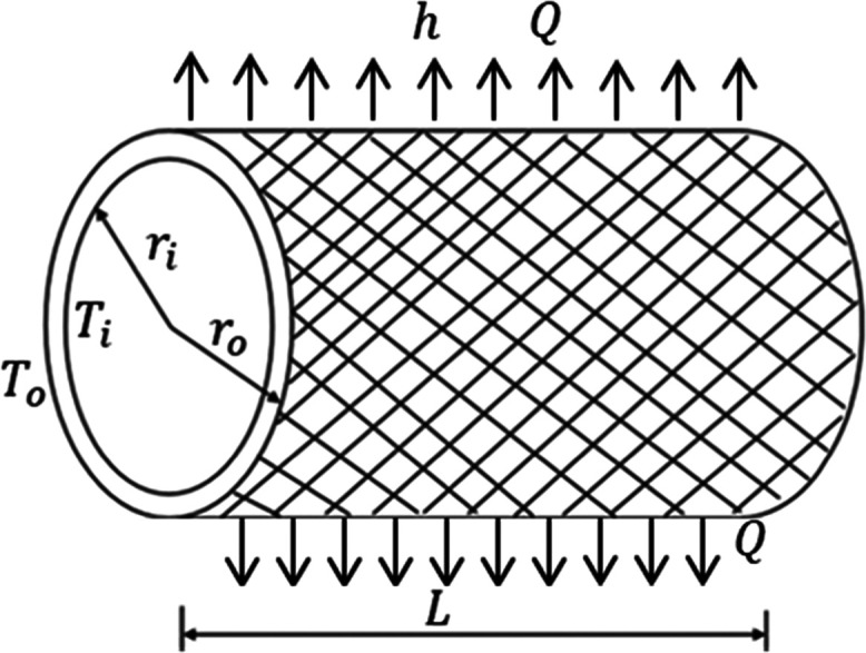
Schematic diagram of insulating material around a cylinder surrounding a heat source.
| 2 |
The steady-state one-dimensional (1D) flow of heat was assumed.60 Thermal conductivity was considered to be constant with temperature, and internal resistance was not considered. The initial guess values for this optimization were taken as k = 1 W/m °C (stage 1) and t = 1 mm (stage 2). The case was investigated in two stages, as stated below:
Stage 1: Insulation material was decided based on its k, optimized for different values of target heat loss (Qo) varying between 91 and 121 W in intervals of 2 W. The outer temperature (To) and inner temperature (Ti) of insulation cylinders were considered as 75 and 500 °C, respectively. The heat source radius was ri = 30 mm. The insulation thickness was 200 mm (or ri = 230 mm). k was subsequently optimized using nonlinear least-squares error (LSE) and linear programming techniques. Accordingly, the heat loss was computed (Qc). Average thermal conductivity (kavg) was computed by the algebraic summation of x1 for all eight considered cases, given in Table 2, divided by 8. The standard insulation material is recommended based on the lowest and average value of k. The fitness function Z1 was minimized using eq 3 by computing x1, which was the unknown thermal conductivity, optimized in the range 0 to 5.
 |
3 |
Table 2. Results for Case 1.
| stage
1 |
stage
2 |
||||||
|---|---|---|---|---|---|---|---|
| Qo (W) | k (W/mK) | Qa (W) | t (mm) | Qo (W) | kavg (W/mK) | Qa (W) | ta (x2) (mm) |
| 91 | 0.069 | 90.46 | 200 | 91 | 0.081 | 91 | 293 |
| 95 | 0.072 | 94.39 | 200 | 95 | 0.081 | 95 | 262 |
| 99 | 0.076 | 99.64 | 200 | 99 | 0.081 | 99 | 237 |
| 103 | 0.079 | 103.57 | 200 | 103 | 0.081 | 103 | 215 |
| 107 | 0.082 | 107.50 | 200 | 107 | 0.081 | 107 | 196 |
| 111 | 0.085 | 111.44 | 200 | 111 | 0.081 | 111 | 181 |
| 115 | 0.088 | 115.37 | 200 | 115 | 0.081 | 115 | 167 |
| 119 | 0.091 | 119.30 | 200 | 119 | 0.081 | 119 | 155 |
| average | 0.08025 | 213.25 | |||||
Stage 2: The thickness of the insulating material was computed for the minimum heat loss given kavg as the maximum thermal conductivity. Insulation thickness was optimized for different values of target heat loss (Qo) varying between 91 and 121 W in intervals of 4 W. To, Ti, and ri were the same as those given in stage 1. t was optimized by considering computed heat loss (Qc) equal to Qo. The fitness function Z2, given in eq 4, was minimized by optimizing x2 (mm), denoting the unknown insulation thickness of the insulation material. The range of optimization was from 0 to 500.
 |
4 |
2.2.2. Case 2: Laminar Airflow on a Heated Plate
The thermal boundary layer thickness was estimated for laminar airflow, where the air characteristics and temperature of the air and plate remained unchanged. Irradiation was neglected. Figure 4 shows a schematic diagram of a flat plate with laminar, turbulent, and transitional regions. Airflow across a hot plate was considered to flow at a specific velocity warmer than that of the air. Airflow in the laminar region was considered. Two separate target variables were computed for this laminar boundary layer problem, subjected to different design variables and constraints, as shown in Table 1. The variable was optimized for the minimum, maximum, and target values. First, the thermal boundary layer thickness (δt) was computed. The second case determined the flow of heat from the plate to air (Q in W). A constant air temperature of 65.6 °C was considered for both problems. Heat flow zone temperature was the mean temperature of air and plate. The air was at atmospheric pressure, whose properties (thermal conductivity (k), air velocity (u∞) in the flow area, density (ρ), and specific heat at constant pressure (cp)) were adopted from Holman.13 The values of these variables may change depending on the plate’s temperature. For problem 1, the initial guess for design variable T was 1 °C, and for x was 1 mm, whereas, for the second case, the design variables began at T = 1 °C, x = 1 mm, and δt = 1 mm.
Figure 4.

Schematic diagram of the laminar flow of air particles over a heated plate.
Table 1. Design Variables and Constraints of Distinct Goals with Two Cases.
| problem | type | goal-range |
|---|---|---|
| 1 | objective | maximum, minimum, and target (19.6 mm) values of δt |
| constraints | Re < 50,000, 140 W < Q < 190 W | |
| design variables | 200 mm < x < 1000 mm, 80 °C < T < 130 °C | |
| 2 | objective | maximum, minimum, and target (160.43 W) values of Q |
| constraints | Re < 50,000 | |
| design variables | 200 mm < x < 1000 mm, 80 °C < T < 130 °C, 0.01 mm < δt < 20 mm, |
The condition for the transition from laminar to turbulent flow is given in eq 5(56)
| 5 |
where x depicts the distance from the leading edge, u∞ depicts the free stream velocity, and ϑ denotes the kinematic viscosity, the ratio of dynamic viscosity (μ) and density (ρ).
The Prandtl number is given in eq 6.56 It has been assumed to be 0.7189 at 69.5 °C. Cp is the specific heat at constant pressure, and α is the diffusivity constant.
| 6 |
The Nusselt number (Nu), for identifying the convective heat transfer for lamellar flow (Re < 5 × 10⁵), is given as eq 7.56
| 7 |
The heat transfer coefficient (h) is given as eq 8.56
| 8 |
The average heat transfer coefficient h̅ is given as eq 9.56Equation 9 is a simplification assumption used to estimate the average heat transfer coefficient in a forced convection environment. It is predicted on the assumption that the local heat transfer coefficient is generally greatest near the plate’s leading edge and decreases as one moves downstream. This assumption is expected to provide a reasonable estimate of the overall heat transfer characteristics of the entire plate.
| 9 |
The heat flow is computed using eq 10,56 where A is the surface area of the plate and T∞ = 65.6 °C and Tw are the temperatures of the fluid outside and at the thermal boundary, respectively.
| 10 |
The hydraulic boundary layer is given in eq 11.56
| 11 |
Thermal boundary layer thickness is given in eq 12.56
| 12 |
The present study solves two cases of this problem. First, thermal boundary layer thickness (δt) is estimated. The second case determines the heat flow from the plate to air (Q in W). The optimization function for conditions 1 and 2 is given in eqs 13 and 14, respectively. Equations 10 and 12 were computed based on optimized variables.
 |
13 |
| 14 |
3. Results
3.1. Nonlinear LSE
3.1.1. Case 1 Heat Loss Optimization from Cylindrical Insulating Surfaces
The results of both stages by nonlinear
LSE are presented in Table 2. For stage 1, model convergence occurred
after 19 iterations. It was found that Qo and Qc values were not significantly
different (Table 2). Figure 5 shows the variation
of the thermal conductivity with heat loss. Results indicate that
the thermal conductivity increased linearly with heat loss (coefficient
of correlation is 0.99). This observation is consistent with eq 2, where Q is inversely proportional to 1/k. In other words, Q is directly proportional to k. kavg value was 0.081 W/mK (Table 1). In the second stage, kavg was taken as constant to determine the optimal thermal
insulation thickness, which decreased with the heat transfer amount
following a decremental logarithmic curve (coefficient of correlation
is 0.99) (Figure 6).
This observation is in accordance with numerical eq 2, where Q is inversely proportional
to 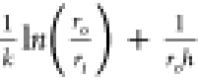 . Considering
  , Q is inversely proportional
to
, Q is inversely proportional
to  . Since ro = ri + t, where t is the insulation thickness
and Q is
inversely proportional to ln(t). Therefore, the relation
will be a logarithmic decrement, as predicted by the optimization
technique.
. Since ro = ri + t, where t is the insulation thickness
and Q is
inversely proportional to ln(t). Therefore, the relation
will be a logarithmic decrement, as predicted by the optimization
technique.
Figure 5.

Variation of thermal conductivity with heat loss.
Figure 6.

Variation of insulation thickness with heat loss.
3.1.2. Case 2 Determination and Optimization of Thermal Boundary Layer Thickness
The case did not fit with the nonlinear LSE due to the unavailability of target data (δt or Q).
3.2. Interior Point Linear Programming Optimization Technique
3.2.1. Case 1 Heat Loss Optimization from Cylindrical Insulating Surfaces
The case needed to compare the target variable to the computed variable. The considered optimization technique does not require a target values. Accordingly, this technique did not predict close results based on the constraints.
3.2.2. Case 2 Determination and Optimization of Thermal Boundary Layer Thickness
Table 3 shows the findings from each condition. When the design factors, average values, and restrictions in conditions 1 and 2 were explored, the findings of issue 2 (Table 3) showed that all readings in the “average” rows in the goal column were not significantly different. Accordingly, the outcomes could be accurately estimated globally even if the impact parameters changed the constraint and design variable.
Table 3. Optimized Values from Case 2 Using a Linear Programming Technique.
| objective | x (mm) | Tw (°C) | Re | δt (mm) | Q (W) | |
|---|---|---|---|---|---|---|
| condition 1 | minimum | 377.3 | 131.89 | 15,001 | 16.9 | 135.14 |
| average | 606.6 | 121.23 | 24,506 | 19.6 | 161.21 | |
| maximum | 907.2 | 108.53 | 41,326 | 24.3 | 598.63 | |
| condition 2 | minimum | 198.6 | 83.20 | 9057 | 18.04 | 12.11 |
| average | 602.1 | 100.01 | 27,222 | 13.74 | 160.40 | |
| maximum | 1010.2 | 127.36 | 40,199 | 0.04 | 601.01 |
4. Discussion
This study aimed to identify a promising optimization technique for two basic heat transfer cases. In the first case, heat loss was minimized through a cylindrical insulating material surrounding a heat source. In particular, optimal thermal conductivity was computed to determine the insulation material, followed by optimal insulation thickness. The average thermal conductivity was 0.081 W/mK, computed using a nonlinear LSE optimization technique. The average thermal insulation thickness was 213.25 mm. These values were generated considering heat loss should not exceed 110 W. tavg was found to be 213.25 mm (Table 1). Akpinar56 performed a similar calculation where GA was employed to determine the optimal insulation thickness for cylinder problems. It was found that kavg was 0.079 W/mK (near to the figure predicted by the nonlinear LSE technique), and optimal material insulation thickness was 141.28 mm, less than predicted by nonlinear LSE. The linear programming technique does not fit this problem. Accordingly, this study stated that the nonlinear LSE optimization technique is better than GA, in that linear programming techniques are not suitable to solve such problems. The slightly higher thermal conductivity significantly influences the rate of heat loss in comparison to the convective heat transfer coefficient.61
For different applications, the optimal insulation thickness was determined in several previous studies. Ndubuisi et al.61 estimated the optimal insulation thickness for a cylindrical ceramic crucible. They found that the increased length of the crucible enhanced its thermal mass, causing it to lose heat at a higher rate.61 Applying more refractories beyond the optimum range will not decrease heat loss considerably and will make the insulating refractory bulkier. Insulation costs rise linearly as insulation thickness increases, whereas energy costs drop. It was also observed that the entire cost, including the cost of energy and insulation, decreased to certain levels of insulation thickness before increasing.62 In summary, other factors such as material cost, a wide range of outer and inner temperatures (depending on the application), time factor, other optimization algorithms, etc., need to be considered and recommended for the investigation of optimal insulation thickness in future studies.
To further support the applicability of nonlinear LSE, case 1 was reinvestigated, considering the initial insulation thickness equal to the average predicted thickness (i.e., 213.25 mm). The final solution was the same as that given in the fourth column of stage 2 of Table 1. This signifies that the technique predicted global optimization.
The optimal thermal boundary layer thickness and heat flow from the plate to the air were also determined in a previous study by using a GA,56 and it was found that results from the applied linear programming optimization technique employed here were very close to GA results published in the previous study.56 During the study, only the nonlinear LSE technique was suitable for estimating optimal insulation thickness and can be recommended for future studies. On the other hand, the linear programming and GA optimization technique was found suitable for determining the optimal boundary layer thickness. It can be recommended for future studies, while the nonlinear LSE technique is unsuitable.
This study has certain limitations. This research compared only three optimization techniques, while other techniques may be better than those to solve the two cases. The nonlinear LSE and programming optimization techniques can also be utilized in more complex heat transfer problems. Other factors, such as material cost, a wide range of outer and inner temperatures (depending on the application), the time factor, and other optimization algorithms (like artificial bee colony, particle swarm optimization, etc.), need to be considered and recommended for the investigation of optimal insulation thickness in future studies.
5. Conclusions
The nonlinear least-squares error optimization technique has been a promising technique to minimize heat loss through a cylindrical insulating material surrounding a heat source. GA is another good technique but less promising than nonlinear LSE to solve such problems. The average thermal conductivity was found to be 0.081 W/mK. The average insulation thickness (tavg) was found to be 213.25 mm. Linear programming and GA are promising techniques for minimizing hot plate airflow, while nonlinear LSE techniques do not fit such problems. The analysis demonstrated that the computations could identify the optimal results in the solution space using an optimization technique. This technique should be wisely selected, as it does not ensure the best solution will be found. It was found that the thermal conductivity increased linearly with increased heat transfer. The boundary layer thickness results indicate that although the target variable is determined, the outcomes could be accurately estimated globally even if the impact parameters change the constraint and design variable.
Acknowledgments
The author thanks the Deputyship for Research and Innovation, “Ministry of Education” in Saudi Arabia, for funding this research (IFKSUOR3-046-2).
The author declares no competing financial interest.
References
- Ozel M. Effect of Insulation Location on Dynamic Heat-Transfer Characteristics of Building External Walls and Optimization of Insulation Thickness. Energy Build. 2014, 72, 288–295. 10.1016/j.enbuild.2013.11.015. [DOI] [Google Scholar]
- Amin M.; Shah H. H.; Fareed A. G.; Khan W. U.; Chung E.; Zia A.; Farooqi Z. U. R.; Lee C. Hydrogen Production through Renewable and Non-Renewable Energy Processes and Their Impact on Climate Change. Int. J. Hydrogen Energy 2022, 47 (77), 33112–33134. 10.1016/j.ijhydene.2022.07.172. [DOI] [Google Scholar]
- Hasanzadeh R.; Azdast T.; Doniavi A.; Lee R. E. Multi-Objective Optimization of Heat Transfer Mechanisms of Microcellular Polymeric Foams from Thermal-Insulation Point of View. Therm. Sci. Eng. Prog. 2019, 9, 21–29. 10.1016/j.tsep.2018.11.002. [DOI] [Google Scholar]
- Vaillancourt K.; Alcocer Y.; Bahn O.; Fertel C.; Frenette E.; Garbouj H.; Kanudia A.; Labriet M.; Loulou R.; Marcy M.; Neji Y.; Waaub J.-P. A Canadian 2050 Energy Outlook: Analysis with the Multi-Regional Model TIMES-Canada. Appl. Energy 2014, 132, 56–65. 10.1016/j.apenergy.2014.06.072. [DOI] [Google Scholar]
- Mekhilef S.; Saidur R.; Safari A. A Review on Solar Energy Use in Industries. Renewable Sustainable Energy Rev. 2011, 15 (4), 1777–1790. 10.1016/j.rser.2010.12.018. [DOI] [Google Scholar]
- Corlu C. G.; de la Torre R.; Serrano-Hernandez A.; Juan A. A.; Faulin J. Optimizing Energy Consumption in Transportation: Literature Review, Insights, and Research Opportunities. Energies 2020, 13 (5), 1115 10.3390/en13051115. [DOI] [Google Scholar]
- Yazdani-Asrami M.; Seyyedbarzegar S. M.; Zhang M.; Yuan W. Insulation Materials and Systems for Superconducting Powertrain Devices in Future Cryo-Electrified Aircraft: Part I—Material Challenges and Specifications, and Device-Level Application. IEEE Electr. Insul. Mag. 2022, 38 (2), 23–36. 10.1109/MEI.2022.9716211. [DOI] [Google Scholar]
- Zaki G. M.; A-T A. M. Optimization of Multilayer Thermal Insulation for Pipelines. Heat Transfer Eng. 2000, 21 (4), 63–70. 10.1080/01457630050144514. [DOI] [Google Scholar]
- Tunçbilek E.; Komerska A.; Arıcı M. Optimisation of Wall Insulation Thickness Using Energy Management Strategies: Intermittent versus Continuous Operation Schedule. Sustainable Energy Technol. Assess. 2022, 49, 101778 10.1016/j.seta.2021.101778. [DOI] [Google Scholar]
- Li T.; Liu Q.; Mao Q.; Chen M.; Ma C.; Wang D.; Liu Y. Optimization Design Research of Insulation Thickness of Exterior Wall Based on the Orientation Difference of Solar Radiation Intensity. Appl. Therm. Eng. 2023, 223, 119977 10.1016/j.applthermaleng.2023.119977. [DOI] [Google Scholar]
- Gaarder J. E.; Friis N. K.; Larsen I. S.; Time B.; Møller E. B.; Kvande T. Optimization of Thermal Insulation Thickness Pertaining to Embodied and Operational GHG Emissions in Cold Climates – Future and Present Cases. Build. Environ. 2023, 234, 110187 10.1016/j.buildenv.2023.110187. [DOI] [Google Scholar]
- Zhang L.; Liu Z.; Hou C.; Hou J.; Wei D.; Hou Y. Optimization Analysis of Thermal Insulation Layer Attributes of Building Envelope Exterior Wall Based on DeST and Life Cycle Economic Evaluation. Case Stud. Therm. Eng. 2019, 14, 100410 10.1016/j.csite.2019.100410. [DOI] [Google Scholar]
- Holman J. P.Heat Transfer, 10th ed.; Mc-GrawHill Higher education: New York, NY, 2010. [Google Scholar]
- Crane D.; Jackson G.; Holloway D. In Towards Optimization of Automotive Waste Heat Recovery Using Thermoelectrics, SAE Technical Paper Series; SAE International: Warrendale, PA, 2001.
- Hao J.-H.; Chen Q.; Hu K. Porosity Distribution Optimization of Insulation Materials by the Variational Method. Int. J. Heat Mass Transfer 2016, 92, 1–7. 10.1016/j.ijheatmasstransfer.2015.08.076. [DOI] [Google Scholar]
- Jaluria Y.Design and Optimization of Thermal Systems, 2nd ed.; CRC Press: Boca Raton, 2007. [Google Scholar]
- Qiao Y.; Liu P.; Liu W.; Liu Z. Analysis and Optimization of Flow and Heat Transfer Performance of Active Thermal Protection Channel for Hypersonic Aircraft. Case Stud. Ther. Eng. 2022, 39, 102476 10.1016/j.csite.2022.102476. [DOI] [Google Scholar]
- Leitmann G.Optimization Techniques: With Applications to Aerospace Systems; Academic Press, 1962. [Google Scholar]
- Bhaskar V.; Gupta S. K.; Ray A. K. Applications of Multi-Objective Optimization in Chemical Engineering. Rev. Chem. Eng. 2000, 16 (1), 1–54. 10.1515/REVCE.2000.16.1.1. [DOI] [Google Scholar]
- Soliman S. A.-H.; Mantawy A.-A. H.. Modern Optimization Techniques with Applications in Electric Power Systems; Springer Science & Business Media, 2011. [Google Scholar]
- Najafi H.; Najafi B.; Hoseinpoori P. Energy and Cost Optimization of a Plate and Fin Heat Exchanger Using Genetic Algorithm. Appl. Therm. Eng. 2011, 31 (10), 1839–1847. 10.1016/j.applthermaleng.2011.02.031. [DOI] [Google Scholar]
- Bidabadi M.; Sadaghiani A. K.; Azad A. V. Spiral Heat Exchanger Optimization Using Genetic Algorithm. Sci. Iran. 2013, 20 (5), 1445–1454. [Google Scholar]
- Shi H.-n.; Ma T.; Chu W.-x.; Wang Q.-w. Optimization of Inlet Part of a Microchannel Ceramic Heat Exchanger Using Surrogate Model Coupled with Genetic Algorithm. Energy Convers. Manage. 2017, 149, 988–996. 10.1016/j.enconman.2017.04.035. [DOI] [Google Scholar]
- Ge Y.; Shan F.; Liu Z.; Liu W. Optimal Structural Design of a Heat Sink With Laminar Single-Phase Flow Using Computational Fluid Dynamics-Based Multi-Objective Genetic Algorithm. J. Heat Transfer 2018, 140, 022803 10.1115/1.4037643. [DOI] [Google Scholar]
- Mekki B. S.; Langer J.; Lynch S. Genetic Algorithm Based Topology Optimization of Heat Exchanger Fins Used in Aerospace Applications. Int. J. Heat Mass Transfer 2021, 170, 121002 10.1016/j.ijheatmasstransfer.2021.121002. [DOI] [Google Scholar]
- Bagherzadeh S. A.; Sulgani M. T.; Nikkhah V.; Bahrami M.; Karimipour A.; Jiang Y. Minimize Pressure Drop and Maximize Heat Transfer Coefficient by the New Proposed Multi-Objective Optimization/Statistical Model Composed of “ANN + Genetic Algorithm” Based on Empirical Data of CuO/Paraffin Nanofluid in a Pipe. Phys. A 2019, 527, 121056 10.1016/j.physa.2019.121056. [DOI] [Google Scholar]
- Zhang T.; Chen L.; Wang J. Multi-Objective Optimization of Elliptical Tube Fin Heat Exchangers Based on Neural Networks and Genetic Algorithm. Energy 2023, 269, 126729 10.1016/j.energy.2023.126729. [DOI] [Google Scholar]
- McCaughtry T.; Kim S. i. Multi-Objective Optimization Tool of Shell-and-Tube Heat Exchangers Using a Modified Teaching-Learning-Based Optimization Algorithm and a Compact Bell-Delaware Method. Heat Transfer Eng. 2022, 43 (13), 1083–1096. 10.1080/01457632.2021.1943836. [DOI] [Google Scholar]
- Wei L.-Y.; Qi H.; Li G.-J.; Zhang W.-J. Improved Teaching-Learning-Based Optimization for Estimation of Temperature-Dependent Radiative Properties of Semi-transparent Media. Int. J. Therm. Sci. 2021, 161, 106694 10.1016/j.ijthermalsci.2020.106694. [DOI] [Google Scholar]
- Khosravi A.; Malekan M.; Pabon J. J. G.; Zhao X.; Assad M. E. H. Design Parameter Modelling of Solar Power Tower System Using Adaptive Neuro-Fuzzy Inference System Optimized with a Combination of Genetic Algorithm and Teaching Learning-Based Optimization Algorithm. J. Cleaner Prod. 2020, 244, 118904 10.1016/j.jclepro.2019.118904. [DOI] [Google Scholar]
- Chau N. L.; Dao T.-P.; Dang V. A. An Efficient Hybrid Approach of Improved Adaptive Neural Fuzzy Inference System and Teaching Learning-Based Optimization for Design Optimization of a Jet Pump-Based Thermoacoustic-Stirling Heat Engine. Neural Comput. Appl. 2020, 32 (11), 7259–7273. 10.1007/s00521-019-04249-y. [DOI] [Google Scholar]
- Kuru M. N. Determination of the Optimum Operating Conditions and Geometrical Dimensions of the Plate Fin Heat Sinks Using Teaching-Learning-Based-Optimization Algorithm. ASME J. Heat Mass Transfer 2023, 145 (6), 063301 10.1115/1.4056299. [DOI] [Google Scholar]
- Rao R. V.; Patel V. Multi-Objective Optimization of Heat Exchangers Using a Modified Teaching-Learning-Based Optimization Algorithm. Appl. Math. Modell. 2013, 37 (3), 1147–1162. 10.1016/j.apm.2012.03.043. [DOI] [Google Scholar]
- Azma A.; Behroyan I.; Babanezhad M.; Liu Y. Fuzzy-Based Bee Algorithm for Machine Learning and Pattern Recognition of Computational Data of Nanofluid Heat Transfer. Neural Comput. Appl. 2023, 35 (27), 20087–20101. 10.1007/s00521-023-08851-z. [DOI] [Google Scholar]
- Bozorgan N.; Ghafouri A.; Assareh E.; Mohammad S. A. S. Design and Thermal-Hydraulic Optimization of a Shell and Tube Heat Exchanger Using Bees Algorithm. Therm. Sci. 2022, 26 (1), 693–703. 10.2298/TSCI210225252B. [DOI] [Google Scholar]
- Daneshgar S.; Zahedi R. Optimization of Power and Heat Dual Generation Cycle of Gas Microturbines through Economic, Exergy and Environmental Analysis by Bee Algorithm. Energy Rep. 2022, 8, 1388–1396. 10.1016/j.egyr.2021.12.044. [DOI] [Google Scholar]
- Gawronska E.; Zych M.; Dyja R.; Domek G. Using Artificial Intelligence Algorithms to Reconstruct the Heat Transfer Coefficient during Heat Conduction Modeling. Sci. Rep. 2023, 13 (1), 15343 10.1038/s41598-023-42536-w. [DOI] [PMC free article] [PubMed] [Google Scholar]
- Yang L.; Sun B.; Sun X. Inversion of Thermal Conductivity in Two-Dimensional Unsteady-State Heat Transfer System Based on Finite Difference Method and Artificial Bee Colony. Appl. Sci. 2019, 9 (22), 4824 10.3390/app9224824. [DOI] [Google Scholar]
- Unal R. E.; Guzel M. H.; Sen M. A.; Kose F.; Kalyoncu M. Investigation on the Cost-Effective Optimal Dimensions of a Solar Chimney with the Bees Algorithm. Int. J. Energy Environ. Eng. 2023, 14 (3), 475–485. 10.1007/s40095-022-00528-y. [DOI] [Google Scholar]
- Bahiraei M.; Foong L. K.; Hosseini S.; Mazaheri N. Neural Network Combined with Nature-Inspired Algorithms to Estimate Overall Heat Transfer Coefficient of a Ribbed Triple-Tube Heat Exchanger Operating with a Hybrid Nanofluid. Measurement 2021, 174, 108967 10.1016/j.measurement.2021.108967. [DOI] [Google Scholar]
- Li L.; Fu Y.; Fung J. C. H.; Qu H.; Lau A. K. H. Development of a Back-Propagation Neural Network and Adaptive Grey Wolf Optimizer Algorithm for Thermal Comfort and Energy Consumption Prediction and Optimization. Energy Build. 2021, 253, 111439 10.1016/j.enbuild.2021.111439. [DOI] [Google Scholar]
- Lara-Montaño O. D.; Gómez-Castro F. I.. Optimization of a Shell-and-Tube Heat Exchanger Using the Grey Wolf Algorithm. In Computer Aided Chemical Engineering; Kiss A. A.; Zondervan E.; Lakerveld R.; Özkan L., Eds.; Elsevier, 2019; Vol. 46, pp 571–576. [Google Scholar]
- Xu Z.; Guo Y.; Yang H.; Mao H.; Yu Z.; Li R. One Convenient Method to Calculate Performance and Optimize Configuration for Annular Radiator Using Heat Transfer Unit Simulation. Energies 2020, 13 (1), 271 10.3390/en13010271. [DOI] [Google Scholar]
- Naser M. Z.Leveraging Artificial Intelligence in Engineering, Management, and Safety of Infrastructure; CRC Press, 2022. [Google Scholar]
- Iyer V. H.; Mahesh S.; Malpani R.; Sapre M.; Kulkarni A. J. Adaptive Range Genetic Algorithm: A Hybrid Optimization Approach and Its Application in the Design and Economic Optimization of Shell-and-Tube Heat Exchanger. Eng. Appl. Artif. Intell. 2019, 85, 444–461. 10.1016/j.engappai.2019.07.001. [DOI] [Google Scholar]
- Kumar G.; Gagandeep; Kumar A.; Ansari N. A.; Zunaid M. Comparative Numerical Study of Flow Characteristics in Shell & Helical Coil Heat Exchangers with Hybrid Models. Mater. Today: Proc. 2021, 46, 10831–10836. 10.1016/j.matpr.2021.01.775. [DOI] [Google Scholar]
- Udayraj; Mulani K.; Talukdar P.; Das A.; Alagirusamy R. Performance Analysis and Feasibility Study of Ant Colony Optimization, Particle Swarm Optimization and Cuckoo Search Algorithms for Inverse Heat Transfer Problems. Int. J. Heat Mass Transfer 2015, 89, 359–378. 10.1016/j.ijheatmasstransfer.2015.05.015. [DOI] [Google Scholar]
- Yan X. Y.; Liang Y.; Cheng G. D. Discrete Variable Topology Optimization for Simplified Convective Heat Transfer via Sequential Approximate Integer Programming with Trust-Region. Int. J. Numer. Methods Eng. 2021, 122 (20), 5844–5872. 10.1002/nme.6775. [DOI] [Google Scholar]
- Wirtz M.; Kivilip L.; Remmen P.; Müller D. 5th Generation District Heating: A Novel Design Approach Based on Mathematical Optimization. Appl. Energy 2020, 260, 114158 10.1016/j.apenergy.2019.114158. [DOI] [Google Scholar]
- Cosic A.; Stadler M.; Mansoor M.; Zellinger M. Mixed-Integer Linear Programming Based Optimization Strategies for Renewable Energy Communities. Energy 2021, 237, 121559 10.1016/j.energy.2021.121559. [DOI] [Google Scholar]
- Gersborg-Hansen A.; Bendsøe M. P.; Sigmund O. Topology Optimization of Heat Conduction Problems Using the Finite Volume Method. Struct. Multidiscip. Optim. 2006, 31 (4), 251–259. 10.1007/s00158-005-0584-3. [DOI] [Google Scholar]
- Liu K.; Tovar A. An Efficient 3D Topology Optimization Code Written in Matlab. Struct. Multidiscip. Optim. 2014, 50 (6), 1175–1196. 10.1007/s00158-014-1107-x. [DOI] [Google Scholar]
- Jalili B.; Mousavi A.; Jalili P.; Shateri A.; Ganji D. D. Thermal Analysis of Fluid Flow with Heat Generation for Different Logarithmic Surfaces. Int. J. Eng. 2022, 35 (12), 2291–2296. 10.5829/IJE.2022.35.12C.03. [DOI] [Google Scholar]
- Cheng D. K. Optimization Techniques for Antenna Arrays. Proc. IEEE 1971, 59 (12), 1664–1674. 10.1109/PROC.1971.8523. [DOI] [Google Scholar]
- Asadi M.; Song Y.; Sunden B.; Xie G. Economic Optimization Design of Shell-and-Tube Heat Exchangers by a Cuckoo-Search-Algorithm. Appl. Therm. Eng. 2014, 73 (1), 1032–1040. 10.1016/j.applthermaleng.2014.08.061. [DOI] [Google Scholar]
- Akpinar M. Application of Genetic Algorithm for Optimization of Heat-Transfer Parameters. Sakarya Univ. J. Sci. 2019, 23 (6), 1123–1130. 10.16984/saufenbilder.500643. [DOI] [Google Scholar]
- Lustig I. J.; Marsten R. E.; Shanno D. F. Feature Article—Interior Point Methods for Linear Programming: Computational State of the Art. ORSA J. Comput. 1994, 6 (1), 1–14. 10.1287/ijoc.6.1.1. [DOI] [Google Scholar]
- Levenberg K. A Method for the Solution of Certain Non-Linear Problems in Least Squares. Q. Appl. Math. 1944, 2 (2), 164–168. 10.1090/qam/10666. [DOI] [Google Scholar]
- Marquardt D. W. An Algorithm for Least-Squares Estimation of Nonlinear Parameters. J. Soc. Ind. Appl. Math. 1963, 11 (2), 431–441. 10.1137/0111030. [DOI] [Google Scholar]
- Cengel Y. A.Heat Transfer: A Practical Approach (No Title).
- Ndubuisi A. O.; Ogunrinola I. E.; Aizebeokhai A. P.; Inegbenebor A. O.; Boyo H. O. Estimation of Optimal Insulation Thickness for a Cylindrical Ceramic Crucible. Int. J. Eng. Res. Technol. 2019, 12 (9), 1389–1393. [Google Scholar]
- Özel M. Determination of indoor design temperature, thermal characteristics and insulation thickness under hot climate conditions. Isı Bilimi Tek. Derg. 2022, 42 (1), 49–64. 10.47480/isibted.1107440. [DOI] [Google Scholar]