A True Score Imputation Method to Account for Psychometric Measurement Error

Abstract

Scores on self-report questionnaires are often used in statistical models without accounting for measurement error, leading to bias in estimates related to those variables. While measurement error corrections exist, their broad application is limited by their simplicity (e.g., Spearman’s correction for attenuation), which complicate their inclusion in specialized analyses, or complexity (e.g., latent variable modeling), which necessitates large sample sizes and can limit the analytic options available. To address these limitations, a flexible multiple-imputation-based approach, called true score imputation, is described which can accommodate a broad class of statistical models. By augmenting copies of the original dataset with sets of plausible true scores, the resulting set of datasets can be analyzed using widely available multiple imputation methodology, yielding point estimates and confidence intervals calculated with respect to the estimated true score. A simulation study demonstrates that the method yields a large reduction in bias compared to treating scores as measured without error, and a real-world data example is further used to illustrate the benefit of the method. An R package implements the proposed method via a custom imputation function for an existing, commonly used multiple imputation library (mice), allowing TSI to be used alongside multiple imputation for missing data, yielding a unified framework for accounting for both missing data and measurement error.

Translational Abstract

All psychological measures, including self-report questionnaires and responses to interviews, contain measurement error; however, these scores are often used in statistical models without accounting for measurement error. While measurement error corrections exist, many require specialized training to implement, reducing their broad utility. To address these limitations, I introduce a measurement error correction, called true score imputation, which uses multiple imputation, allowing it to accommodate a broad class of statistical models. A simulation study demonstrates that the method yields a large reduction in bias compared to treating scores as measured without error, and a real-world data example is further used to illustrate the benefit of the method. True score imputation is currently implemented by piggybacking on existing multiple imputation software available in the free statistical platform R, allowing true score imputation to be combined with multiple imputation for missing data. The resulting imputed data sets can be analyzed within R using existing convenience functions or imported into other software programs such as SAS or Mplus which can analyze multiply imputed data. This method and its implementation allow measurement error to be more easily accounted for in statistical analyses involving psychological measures, improving the accuracy of statistical results.

Psychology researchers cannot measure many variables of interest directly, including those related to a participant’s mental state or emotional, social, or behavioral traits. Instead, researchers use psychometric instruments to measure these variables, but it is well-understood that all such measures are imperfect and that their scores, which I call observed scores or simply scores, reflect both measurement error and a score that would have been observed had there been no measurement error, which I call the true score in keeping with classical test theory (CTT) terminology for the same. As such, virtually all instruments are examined for reliability, often defined as the proportion of variance in the observed score which reflects the true score. In practice, reliability is always less than perfect, even on lengthy and well-constructed measures. If the observed score is treated as error-free, bias is introduced in estimates of relationships with other variables, with compounding effects when multiple variables are measured with error. This bias permeates psychological, sociological, and biomedical research because psychometric instruments, including performance and self- and proxy-report measures, are often used to measure variables of interest. Methods to correct for this bias benefit all such research.

One class of corrections that has potential for broad application is to treat the unobserved variable of interest as missing data and apply methods such as multiple imputation (Rubin, 1987; see also Enders, 2010) for missing data. This idea is not new in psychometrics (Mislevy, 1991) or other fields (e.g., MIME; Cole, Chu, & Greenland, 2006; Ghosh-Dastidar & Schafer, 2003; Winkler, 2003; Guo, 2010; Guo, Little, & McConnell, 2012; Keogh & Bartlett, 2021). Mislevy (1991, Example 1) originally proposed constructing multiple imputations from observed scores and a reliability estimate in the complete-data case within the framework of CTT. Mislevy’s method is currently implemented in the miceadds package (Robitzsch & Grund, 2022) in R (R Core Team, 2022) via the mice.impute.plausible.values function but has not been generalized to account for missing data alongside imputation of one or more true scores. Blackwell et al. (2017) proposed a similar technique to Mislevy, operating from observed scores and reliability or standard error of measurement estimates and currently implemented in the Amelia package in R (Honaker, King, & Blackwell, 2011), but is similarly limited. Clarification on how imputation of true scores from observed scores can be properly combined with imputation of missing values of observed scores, observed variables (i.e., those assumed to be error-free), or both, will bridge this gap in software and literature.

In this work, I synthesize imputation of latent variables as described in Mislevy (1991, Example 1) with methods from bioassay research (Guo, 2010; see also Guo, Little, & McConnell, 2012) and multiple imputation statistical theory to construct proper imputations of the true score using only observed scores and reliability estimates in a broader multiple imputation framework. I also show how applying some simple analytic transformations to Mislevy’s Example 1 enable imputation from scores generated via item response theory (IRT) and accommodate differential measurement error across the latent variable range. The ability to use IRT-generated scores allows researchers to benefit from measurement error correction when working with externally estimated latent variable scores and standard errors, such as those provided by a third-party scoring service like the HealthMeasures (2022) Assessment Center Scoring Service which can score PROMIS^®, NIH Toolbox, and NeuroQOL instruments or large-scale achievement tests which produce IRT scores (Masters et al., 1990; Cohen et al., 1989; Wandall, 2011). More broadly, it allows a statistician to separate the scoring, measurement error correction, and analysis phases of a statistical pipeline, allowing greater flexibility in each.

This method, called true score imputation (TSI), results in multiple completed datasets that can be analyzed using multiple imputation pooling methods (Rubin, 1987; Enders, 2010). Importantly, the proposed method does not require latent variable modeling on the part of the end user, making it much more broadly applicable when secondary analysis is conducted on already-generated observed scores. Also, unlike many analytic methods for correcting for measurement error, such as Spearman’s (1904, 1910) correction for attenuation or solutions to the errors-in-variables problem in the generalized linear model (Caroll, 1989), the imputations generated by the proposed method can be used in a wide variety of subsequent analyses without the need for complicated analytical derivations and/or programming of already-derived equations to propagate measurement error forward in the analysis pipeline. Accompanying this article, I provide an R package, TSI, that piggybacks on the mice package (van Buuren & Groothuis-Oudshoorn, 2011) to allow readers to combine TSI with multiple imputation for missing data in an existing software framework.

In this manuscript, I first review existing tools that account for measurement error, including analytical corrections, latent variable modeling, plausible value imputation from an IRT model, and factor score regression, and clarify the position of imputation-based approaches within this literature. Next, I provide a brief overview of multiple imputation methodology and describe how missing information principles of multiple imputation can be straightforwardly generalized to include measurement error. I then describe TSI in detail and compare the performance of TSI to the approach of ignoring measurement error in a large simulation study. Lastly, I present a real-world example using data from the PROMIS Profiles-HUI data (Cella, 2017), a publicly available dataset containing measures from the Patient-Reported Outcomes Measurement Information System (PROMIS^®), demonstrating the results of correcting for measurement error in practice.

Psychometric Measurement Error Corrections

Many measurement error corrections have been proposed. Spearman (1904, 1910) proposed a correction for attenuation which accounts for measurement error by using reliability estimates to re-scale the correlation between two tests. Similar analytic methods have been proposed to account for measurement error in the generalized linear model; see Caroll (1989) for a review. Despite continued arguments for application of these techniques (e.g., Schmidt & Hunter, 1999; Jurek et al., 2006), resistance still exists to their broad application, either due to concerns about artificially “inflating” or “exaggerating” effects or because it is not always clear how to incorporate such corrections into complex analysis pipelines. Like analytical corrections, TSI operates from score and reliability (or, as will be shown, standard error of measurement) estimates and makes strong, but testable, assumptions regarding the measurement properties of the instrument used, including the reliability of its observed scores and the plausibility of the measurement model used to generate them. Thus, as with analytical corrections, TSI in its most straightforward application is most useful for unidimensional constructs with trustworthy validation studies where its assumption that the provided reliability estimate is valid is most likely to hold.

The most common contemporary argument against analytical corrections like Spearman’s is that it is generally better to analyze psychometric data using latent variable modeling, treating items as indicators of a latent trait, rather than analyzing summary scores (Borsboom & Mellenbergh, 2002). The most important advantage is that latent variable modeling, including factor analysis and IRT, allows the statistical assessment of the psychometric properties of an instrument within the assessed population, including (uni)dimensionality of data, measurement invariance, construct validity, and model fit. Critically examining these features is highly valuable, especially when the measure or its properties in a target population are not well-studied, and I agree with Borsboom and Mellenbergh (2002) in advocating for the application of latent variable modeling when feasible.

That said, latent variable modeling is statistically more complex than analytic transformations of correlation coefficients (e.g., Spearman’s) or simply ignoring measurement error. This complexity results in a higher training barrier to conducting the analysis, restriction of the types of analyses that can be conducted, and an increase in the complexity involved in specifying, estimating, and interpreting virtually any statistical model. Latent variable modeling also requires large sample sizes to obtain reliable estimates, especially when many variables are included or when the model adds more complicated features (multiple groups, latent mixtures, other random effects, etc.). While continuing developments in latent variable modeling are steadily chipping away at the set of applications for which these constraints present obstacles (e.g., Bentler & Yuan, 1999,; Deng, Yang, & Marcoulides, 2018; Devlieger et al., 2016) there remains a need for a variety of broadly applicable methods to correct for measurement error, especially when other approaches, such as latent variable modeling, are untenable. By operating from the score level instead of the item response level, TSI has lower sample size requirements than latent variable modeling; as the included simulation will show, TSI has strong performance even in sample sizes as low as 50. This is made possible by outsourcing the latent variable modeling from the main analysis: TSI operates on scores generated from already-calibrated item parameters, such as those obtainable from IRT analysis, but this analysis does not necessarily need to be conducted by the analyst using the scores. Like latent variable modeling, TSI requires some understanding of a specialized statistical area, namely multiple imputation. This renders TSI a complementary approach to these methods, allowing researchers flexibility in selecting their approach based on their background, expertise, and the constraints of their desired analysis pipeline which may be more amenable to one approach over the other. As a final note, given the endemicity of missing data, researchers are likely to require some method of missing data handling in practice, and one advantage of TSI is its ability to piggyback on multiple imputation for missing data, allowing an analyst to solve both problems at once.

Two additional approaches are also worth mentioning due to their similarity to TSI. First, correcting for measurement error using observed scores and standard errors in TSI resembles factor score regression, a hybrid of analytical corrections and latent variable modeling in which an analysis involving latent variables is conducted in two steps: a scoring step, in which latent variable estimates (observed scores) are obtained for each individual; and an analysis step, in which those scores are used in more complex models. Recent developments have enabled sophisticated analytical measurement error corrections within the structural equation modeling framework (Devlieger et al., 2016). This solves for generalizing analytic corrections to more complex models, but only partially, as these tools are currently only available for structural equation models in the analysis step. TSI, like factor score regression, separates the scoring and analysis steps, but represents measurement error using multiple imputed data sets rather than using analytical methods to pass measurement error to the analysis step. This provides greater flexibility for TSI because the generated imputations can be incorporated into any complete-data analysis compatible with multiple imputation, including but not limited to structural equation models; and the scoring step does not need to be done by the analyst themselves, who can work with already-generated scores and standard errors. For newer measures or those administered to unique samples where validation evidence is not as strong, TSI can be used in a multi-step procedure like factor score regression, allowing detailed latent variable modeling in the measurement step, compatibility with multiple imputation for missing data in the imputation step, and a wider variety of models in the analysis step.

Second, another proposal from Mislevy (1991), namely plausible value imputation (see also Asparouhov & Muthén, 2010) is a hybrid of multiple imputation and latent variable modeling and has been used fruitfully in analyzing data from large-scale assessments (e.g., Beaton & Gonzales, 1995). In this approach, an estimated IRT model is used to generate, for each individual, multiple draws from the posterior distribution of each latent variable given the observed item responses, yielding a set of plausible (hence the name) latent variable values. As with imputed true scores in TSI, these plausible values are then augmented to the original data set, yielding a set of plausible completed data sets on which complete-data analyses can be run, yielding multiple sets of analytical results which are combined using multiple imputation pooling rules (Rubin, 1987; see also Enders, 2010). The major drawback of plausible value imputation is its use of an IRT model, which must include all relevant covariates, on the part of the analyst to generate the imputations. TSI generates plausible imputations from scores and reliability or standard error estimates only, bypassing this latent variable modeling step while still properly accounting for other observed variables.

A Brief Overview of Multiple Imputation

The proposed TSI algorithm resembles multiple imputation for missing data. Therefore, before presenting the method in detail, I begin with an overview of multiple imputation. For a more detailed explanation, readers can refer to Rubin (1987) and Enders (2010). To first clarify terminology, both observed scores (measured with error) and observed variables (measured without error or assumed as such) can have missing values, referring to observation-by-variable elements of the data matrix where no data are available.

Consider a sample containing missing values but with no measurement error. If the pattern of missing data is assumed to be either completely random (missing completely at random, or MCAR) or predictable from other variables in the dataset (missing at random, or MAR), it is possible to derive a posterior distribution of values that would have been observed in place of the missing data. Let $X_{miss}$ denote the missing data, and let $X_{obs}$ denote observed data, such that a hypothetical complete dataset, which I write as $\left[X_{miss};X_{obs}\right]$, could be constructed by combining the two. Then, under the less-restrictive MAR assumption, the conditional distribution of the missing data given the observed data can be written as, from (Rubin, 1987, p. 161)

$$\begin{array}{c}p\left(X_{miss}|X_{obs}\right)=\int p\left(X_{miss}|X_{obs},\theta \right)p\left(\theta \right|X_{obs})d\theta \end{array}$$ (1)

In words, the conditional distribution of the missing data given the observed data can be found by integrating with respect to the parameter vector $\theta$ of the probability distribution assumed to underly the joint distribution. Under the MAR assumption, this conditional distribution can be derived from the observed data, and thus this integral is estimable. If the missing data cannot be predicted from the observed data (for instance, when missingness is caused by variables that are unavailable), then the data are considered missing not at random (MNAR) and very strict a priori assumptions are required to derive this distribution. A more detailed discussion of missingness mechanisms, can be found in Enders (2010, chapter 1).

Multiple imputation is one method for analyzing data when the missingness mechanism is MCAR or MAR. In multiple imputation, multiple draws of $X_{miss}$ are taken from its conditional distribution, yielding $m$ completed datasets constructed by augmenting the observed data with the sampled values of the missing data. The key part of this process is the derivation of the conditional distribution $p\left(X_{miss}|X_{obs},\theta \right)$ of the missing data given the observed data and some parameter vector $\theta$. In multiple imputation, this conditional distribution can be derived using Markov Chain Monte Carlo (MCMC; Gelman et al., 1995), multiple imputation by chained equations (MICE¹; van Buuren & Oudshoom, 1999) or the EM algorithm (Dempster, Laird, & Rubin, 1977; Blackwell, Honaker, & King, 2017), each of which accounts for uncertainty in $\theta$ slightly differently.

Because the current implementation of TSI relies on the MICE algorithm, I must briefly explain its mechanics. In MICE, each imputation is generated using a series of predictive algorithms for each imputed variable. First, missing data are filled in with random values, yielding a less-than-plausible completed dataset of starting values. Then, each variable’s values are updated using a predictive model for that variable based on all other variables included in the dataset, where parameters $\theta$ of the predictive model are sampled from their respective asymptotic sampling distribution or posterior distribution. After predicting each variable, its predicted values are used to predict subsequent variables, producing the eponymous chain of equations. After enough steps, the imputed values represent a draw from the above distribution. Repeating this process with $m$ sets of starting values, or sampling intermittently $m$ times from a single, long chain of predictions, yields multiple completed datasets for use in subsequent analysis.

Regardless of the imputation method used, multiple imputation results in $m$ plausible completed datasets ${X_{complete}}^{(m)}=[{X_{miss}}^{(m)};X_{obs}]$. The term “plausible” must be used as a caveat when referring to imputed datasets because complete datasets were not observed. Instead, under the MAR or MCAR assumptions, the completed datasets represent configurations of the complete dataset which are statistically consistent with the observed data. Differences between values of ${X_{miss}}^{(m)}$ across the $m$ completed datasets represent the analyst’s uncertainty in estimating the values that would have been observed if no data were missing. In short, multiple imputation does not “make up data” and treat it as observed, but rather uses information from the observed data to conduct analyses despite the presence of missing data, using imputations as an intermediate step to allow the use of statistical frameworks, such as ordinary least squares regression, which require complete data.

Once the completed datasets are generated, each can then be analyzed according to the researcher’s chosen statistical model, yielding $m$ sets of parameter estimates and standard errors, one from each of the $m$ completed-data analyses. The parameter estimates from each of the $m$ sets of results can be treated as draws from their associated posterior distribution and averaged to yield a point estimate of the parameter of interest and imputation-specific standard errors can be combined with the between-imputation variability in estimates to yield statistically sound standard errors that account for the fact that some data were not observed. Rubin (1987) outlined a set of simple algebraic pooling rules which can be used to aggregate the sets of estimates and standard errors, yielding a single set of results for interpretation.

Measurement Error as a Missing Information Problem

Blackwell, Honaker, & King (2017; see also Mislevy, 1991) describe a conceptual framework for using multiple imputation to account for measurement error based on the conceptualization by Dempster, Laird, & Rubin (1977) of latent variable modeling as a missing data problem. The core principle is that measurement error represents an intermediate point on the continuum between complete data, which provide complete information on the variables of interest for the associated observation, and the missingness of data entirely, which yields no information on the variables of interest. To illustrate this concept, consider a variable $x$ which is of scientific interest. Instead of $x$, an investigator may observe a variable $w$ which is defined by adding random noise to $x$ according (Blackwell, Honaker, & King, eq. 1):

$$\begin{array}{c}w=x+u,u~N\left(0,{\sigma }_u^2\right)\end{array}$$ (2)

Readers familiar with CTT will immediately recognize this as the equation defining the relationship between the observed score $w$ and the true score $x$ within that framework.

A multiple imputation model in the style of Rubin (1987) treats all values of ${\sigma }^{2}u$ as equal to either zero for observed values, indicating that a variable was measured without error, or infinity for missing values, indicating that no information is available. Measurement error simply represents the same equation with intermediate values of ${\sigma }^{2}u$. Conceptualizing measurement error as a special case of statistical analysis with missing data raises the prospect of using the same statistical framework for both.

Next, consider a dataset containing no missing data but containing one or more variables measured with error (i.e., observed scores). In practice, these are typically multi-item measures whose responses are combined to form a summary score on the measure, for example by summing or averaging item responses or using a psychometric model such as an IRT model to generate scores. Then, a hypothetical completed dataset, which would permit the assessment of relationships involving the underlying true scores, would consist of the original dataset augmented by variables $X_{true}$ corresponding to the underlying true scores. Then, completed datasets can be generated if the following distribution can be derived, by the logic of (1):

$$\begin{array}{c}p\left(X_{true}|X_{obs}\right)=\int p\left(X_{true}|X_{obs},\theta \right)p\left(\theta |X_{obs}\right)d\theta \end{array}$$ (3)

This integral is identical to (1) but exchanges missing data for true scores, treating the latter as a special case of the former. In practice, this involves adding a variable to a data set, starting with random or missing values depending on implementation, and imputing all values of this variable.

As with multiple imputation for missing data, the key step is identifying the conditional distribution $p\left(X_{true}|X_{obs},\theta \right)$. If such a distribution is available, then (3) can be applied to yield proper imputations of $X_{true}$. As with multiple imputation, completed datasets can be analyzed separately and combined using multiple imputation pooling rules.

If, in addition, some values of observed variables, including but not limited to observed-score variables, are missing, then the following joint distribution of the missing data and true scores is required:

$$\begin{array}{c}p\left(X_{true},X_{miss}|X_{obs}\right)=\int p\left(X_{true},X_{miss}|X_{obs},\theta \right)p\left(\theta |X_{obs}\right)d\left(\theta \right)\end{array}$$ (4)

This result follows from (1) and the aforementioned link between measurement error and missing data. However, note that this integral can be estimated by piggybacking on the MICE algorithm, alternating draws from the following two distributions:

$$\begin{array}{c}p\left(X_{miss}|X_{obs},X_{true}\right)=\int p\left(X_{miss}|X_{obs},X_{true},{\theta }_{miss},{\theta }_{true}\right)p\left({\theta }_{miss}|X_{obs},X_{true},{\theta }_{true}\right)d\left({\theta }_{miss}\right)\end{array}$$ (5a)

$$\begin{array}{c}p\left(X_{true}|X_{obs},X_{true}\right)=\int p\left(X_{true}|X_{obs},X_{miss},{\theta }_{miss},{\theta }_{true}\right)p\left({\theta }_{true}|X_{obs},X_{miss},{\theta }_{miss}\right)d\left({\theta }_{true}\right)\end{array}$$ (5b)

Here, the parameter vector $\theta$ is separated into two components: ${\theta }_{miss}$, containing parameters of the model used to impute missing data; and ${\theta }_{true}$, containing parameters of the model used to impute the true scores. The integral is taken with respect to each in turn when deriving the distribution for the other corresponding data component (e.g., integrating with respect to ${\theta }_{miss}$ to obtain a conditional distribution for $X_{true}|X_{obs},X_{miss}$. In practice, as in the MICE algorithm, $X_{true}$ and $X_{miss}$ are initialized with random or missing values, depending on implementation, and each is imputed in turn conditional on previously-imputed values of the other, iterating until convergence. Thus, simultaneous multiple imputation of true scores and missing data merely requires augmenting existing methods for imputing missing data given observed data (5a) with a method for imputing true scores, given observed scores (5b). In the next section, I present a method for the latter.

True Score Imputation (TSI)

As is well-known in multiple imputation (see Enders, 2010) and in plausible value imputation (Mislevy, 1991), if the imputation model for a variable does not include variables used in subsequent analysis, then the generated imputations will not properly reflect the joint distribution of the imputed variable with those variables, yielding bias in subsequent analysis. Using the notation above, deriving a statistically proper distribution $p(X_{true}|X_{obs},X_{miss},{\theta }_{true})$ requires incorporation of all the information in the observed data, not just the information in the observed score(s) associated with the true score(s). Thus, TSI requires deriving an equation predicting the true score from the observed score and other variables in the imputation model to generate proper imputations.

Deriving this equation involves combining two other equations: a multivariate regression equation predicting all other variables in the imputation model from the observed score, which can be readily derived in practice because all variables involved are observed, and a regression equation predicting the true score from the observed score. For CTT, the second equation is a function of test reliability; for IRT-based scoring, as will be shown, similar equations can be derived using the estimated standard errors of measurement for each score. Once these two equations are obtained, they can be combined using the SWEEP operator (Goodnight, 1979; Dempster, 1969) to yield the full prediction equation for the true score. Armed with these equation, one can sample plausible true score values.

In the next section, I present a true score prediction equation as well as analogues for expected a posteriori (EAP) and maximum likelihood (ML) IRT scoring. Next, I provide an overview of the SWEEP operator and relevant assumptions of TSI, followed by a description of the implementation of TSI using the infrastructure in the mice package.

General equations predicting true scores from observed scores

For true score $X$ and observed score $W$ with arbitrary but equal means ${\mu }_X={\mu }_W$, arbitrary true score variance ${{\sigma }^2}_X$,, and squared reliability coefficient ${\rho }^2={{\sigma }^2}_X/{{\sigma }^2}_W$, the regression equation predicting $X$ from $W$ and the associated residual variance are given by (Kelley, 1927; Mislevy, 1991):

$$X={\rho }^{2}W+\left(1-{\rho }^2\right){\mu }_W+e_X;e_X~N(0,{\sigma }_{X|W}^2).$$ (6)

Note that the expected value of the true and observed scores is assumed to be identical due to $\mathrm{E}\left(e_x\right)=0$, but any given observed score will be biased towards the mean (Kelley, 1927). Note that the reliability estimate ${\rho }^2$ is likely not the same as that obtained in the calibration sample because the variances of scores may differ between samples; see Supplemental Methods for more details and for information on the estimation of the conditional variance ${{\sigma }^2}_{X|W}$. Also note that this equation also relies on the observed score $W$ being a perfectly valid measure of $X$ or, equivalently, only yields imputed true scores with the same validity as $W$.

Reliability estimation for CTT.

A crucial component of (6) is the reliability coefficient ${\rho }^2$. One estimate of ${\rho }^2$ which is routinely calculated during test development is coefficient alpha $\left(\alpha \right)$, or the average of all possible split-half correlations. If the item set is treated as fixed, $\alpha$ is typically an underestimate of ${\rho }^2$ (Guttman, 1945, p. 274), and using $\alpha$ in TSI will likely over-correct for measurement error. Rather, for a fixed item set, the glb, which represents the smallest reliability possible given an observed covariance matrix (Bentler & Woodward, 1980; Jackson & Agunwamba, 1977; Woodhouse & Jackson, 1977), is widely available in software and serves as a better lower-bound estimate of reliability. If no model-based estimate of reliability is available, it is preferable to compare the results of TSI with reliability equal to the glb to TSI with reliability equal to one, considering both as plausible, than to simply calculate $\alpha$, or obtain it from the sample used to obtain validity evidence for the scale’s scores, and treat it as a reliability estimate for TSI. In general, whether $\alpha$ or any other estimate is suitable for use in TSI depends on whether it was estimated under the proper assumptions (parallel tests, tau-equivalence, congeneric, etc.). Numerous estimators from latent variable modeling have been proposed which make their own assumptions about the data-generating model; see Revelle & Zinbarg (2009) for a detailed treatment and comparison of these estimators. Lastly Ellis (2021) distinguished between a fixed item set and a random item set, wherein the latter assumes the observed items are sampled from a population of similar items, and noted that, in the typical case where a single sample of responses to a single item set is collected, $\alpha$ is a reasonable lower bound estimate for reliability if the item set is treated as random, in which case its use in TSI is justified. A discussion of the plausibility of treating the item set as fixed or random is beyond the scope of this work; see Ellis and Sijtsma & Pfadt (2021) for a detailed treatment.

Whichever estimator is used, the statistical validity of TSI in the CTT context depends first and foremost on whether the CTT model in Equation (2) applies in the first place. Contemporary applications, under the framework of generalizability theory (e.g., Brennan, 1992), decompose observed score variance into components beyond simply true scores and independent error and are likely closer to a true representation of the data. Extensions of TSI to generalizability theory is outside the scope of this work.

Item response theory.

In IRT, the probability of a given response to a categorical item or set of items is related through (usually nonlinear) functions to the latent variable measured by the item(s). Numerous IRT models exist, and one of the most general and widely used is the graded response model (GRM; Samejima, 1968) which includes the one- and two-parameter logistic models as special cases. If such an IRT model has adequate model fit and represents a plausible data-generating model, score estimates and associated standard errors of measurement can be obtained for each respondent.

Three methods for IRT-based scoring are considered here: maximum likelihood (ML) and expected (EAP) and maximum (MAP) a posteriori. All three scoring methods yield two values for each scored response pattern: the score estimate itself and an individual-level standard error estimate which quantifies measurement error as uncertainty in the value of the obtained score, similarly to ${{\sigma }^2}_E$ in CTT.

While the same general equation (6) can be used to predict true scores (here, latent variable values) from observed scores in IRT, the nonlinear nature of IRT complicates the estimation of the mean and variance of the latent variables. Specifically, ML scores are biased estimates of true scores as a function of the slope parameters (Lord, 1986, Equation 6), which are often proprietary information not available to analysts. However, if the likelihood function of the latent variable given the observed item responses is assumed to be normal, then these parameters can be estimated from the score estimates and standard error estimates based on derivations in Mislevy et al. (1999) and Lord (1986).

In particular, given this assumption, the expectation of the ML estimates is equal to the expectation of the true scores $\left({\mu }_X={\mu }_W\right)$, and the variance of the true scores is equal to (Mislevy et al., pp. 138):

$$\begin{array}{c}{\sigma }_X^2={\sigma }_W^2-S{E}^2\end{array}$$ (7)

where $SE$ is the estimated standard error for the ML estimate. Reliability in the analysis sample is then estimated as

$$\begin{array}{c}{\rho }^2=\frac{{\sigma }_X^2}{{\sigma }_W^2}\end{array}$$ (8)

Note that these equations are nearly identical to their corresponding equations in CTT: the true score variance is calculated by subtracting an error variance from the observed score variance, and reliability is the ratio of true to observed score variance. These terms can then be used in Equation (6) to yield true score prediction equations for ML score estimation.

If a standard normal prior is used, as is done in HealthMeasures (2022) for example, Lord (1986; Eq. 7) provide an estimate of the difference between ML and MAP as $X/I$, where $X$ is the MAP score estimate and $I=S{E}^2-{{\sigma }^2}_P$, where $S{E}^2$ is the squared MAP standard error and ${{\sigma }^2}_P$ is the variance of the prior used for scoring. If this prior is a standard normal distribution, then this variance equals one and the resulting EAP or MAP estimates are further biased towards the mean than ML. Similarly, the square root of $1/I$ provides an estimate of the standard error that would have arisen from ML scoring by removing the influence of the prior from the MAP standard error. Using these values, each MAP estimate and standard error can be converted to an estimated ML estimate and standard error, removing the additional bias added by the prior, after which (7) and (8) can be derived and substituted into (6) to derive a regression equation predicting the true score from the transformed MAP estimates. Carrying through the same assumption of normally distributed likelihood and posterior distributions mentioned earlier, MAP and EAP estimates and standard errors become equivalent because the mean and mode of a normal distribution are identical, and thus the same equations can be used to transform EAP estimates and standard errors to approximate corresponding ML values for use in TSI. The resulting “pseudo-ML” estimates differ from ML both in their calculation, which involves a two-step process and a normal posterior distribution assumption, and because, unlike ML estimates, they can be calculated even if all item responses are in the highest and lowest response categories for the graded response model.

Standardized metrics of observed scores.

In practice, the scaling of observed scores in the calibration sample is often specified by the test creators. For instance, IQ scores are constructed in such a way that the mean score in the calibration sample is 100 and the standard deviation is 15; scale scores for the Wechsler IQ tests are constructed such that the mean score in the calibration sample is 10 and the standard deviation is 3; and HealthMeasures instruments, including PROMIS, NIH Toolbox, and NeuroQOL measures, use a T-score metric with a mean of 50 and standard deviation of 10. However, all of these scores can be converted to the standard normal metric ($z$ scores) by subtracting the metric’s mean (100, 10, and 50 for IQ, scale, and T scores, respectively) and then dividing by its standard deviation (15, 3, and 10, respectively), while standard errors can be converted to the standard normal metric by dividing by the metric’s standard deviation. Thus, a TSI algorithm does not need to operate on arbitrary score metrics per se but can instead be provided the score metric when executed, convert the observed scores to $z$ scores, perform the imputation, then convert the imputed scores back to the original metric.

Differential measurement error.

In IRT, the individual-level standard error, which is related to reliability through (7), differs as a function of the item response patterns. In general, reliability is higher for response patterns which yield latent trait estimates close to the region of maximal test information and for response patterns with fewer missing responses. For a fixed number of items, the TSI algorithm defined herein can be adapted to account for these differences in measurement error across individuals by calculating (7) separately for each unique reliability estimate, calculated from each unique standard error estimate from IRT scoring, and allowing the TSI model in (6) to differ for each unique reliability estimate. While this is more computationally demanding than using a single reliability estimate for the entire sample, it may yield more accurate imputations when reliability differs greatly across observations. A demonstration of TSI’s ability to account for IRT’s inherent heteroscedastic measurement error is included in Supplemental Simulation.

Deriving the Imputation Model

The SWEEP operator (Goodnight, 1979; Dempster, 1969; see also Schafer, 1997; Little & Rubin, 2014) can be used to predict the true score from the observed score and other analysis variables by combining two linear regression equations: the equation predicting the true score from the observed score, as derived in the previous section; and the multivariate regression equations predicting each observed variable from the observed score. Details on the application of the SWEEP operator to TSI can be found in Supplemental Methods, and readers can refer to the above sources for more comprehensive treatments.

One consideration when using the SWEEP operator in TSI is its reliance on the assumption of non-differential measurement error (NDME); that is, that measurement error is statistically independent of other variables in the imputation model given the true score. If the observed score being analyzed reflects only the combination of meaningful variance on a single latent domain and statistical uncertainty that is independent of all other variables in the imputation model (“true error”), then the NDME assumption holds. In psychometric applications, sources of variance other than the true score and true error can arise from violations of unidimensionality when nuisance dimensions are correlated with other variables in the imputation model. For shorter measures, violations of NDME can arise when unique but reliable variance components from individual indicators of the latent variable, for example raw item responses to a multi-item measure, are meaningfully related to the other variables in the imputation model. Both assumptions can be tested through latent variable modeling of the indicators themselves: dimensionality violations by bifactor analysis to identify reliable sources of variance beyond a general factor spanning the entire measure (e.g., coefficient omega hierarchical; McDonald, 1999), and reliable specific variance by methods such as those described in Bentler (2017) which estimate such variance components directly.

To summarize this section, the TSI algorithm proceeds as follows:

1. Estimate a regression model predicting the observed scores from the other variables of interest in the imputation model.

2. Construct a regression model predicting true scores from observed scores using the mean and variance of observed and true scores and an estimate of the squared reliability coefficient or the standard error of observed scores (Equation 6). If separate reliability or standard error estimates are available for each set of variables, separate regression equations can be derived for each unique estimate.

3. Use the SWEEP operator to derive a regression equation predicting the true score from the observed score and other variables in the imputation model.

4. Generate predicted values of the true score for each observation using the equation derived from step 3. In the TSI package, these true scores are placed in a new column within the data set.

5. Repeat steps 1 to 4 multiple times to generate multiple completed datasets containing plausible true score values.

6. Analyze the completed datasets separately using the analysis model of interest, using the imputed true score in place of the observed score.

7. Use multiple imputation pooling rules (e.g., Rubin, 1987; Enders, 2010) to aggregate the statistical results of each analysis, yielding a single set of statistical results.

The TSI and mice Packages

A key benefit of using multiple imputation to account for measurement error is the potential for combination of missing data and TSI, which allows an analyst to correct for measurement error and missing data simultaneously. As already described, algorithms for imputing missing data given observed data are well-established. These methods are implemented in multiple software programs, including R (mice package; van Buuren & Groothuis-Oudshoorn, 2011), SAS (proc mi), Mplus (Muthén & Muthén, 1998–2017), and Blimp (Enders et al., 2018), to name a few.

The mice package in R allows the user to specify custom imputation functions and provide additional data with which to generate imputations. This functionality makes it an ideal system in which to implement TSI because, not only are many additional packages available for pooling and analyzing the results of data imputed using mice (e.g., semTools for structural equation modeling; Jorgensen et al., 2021), but also because TSI can be combined with multiple imputation within the same mice function call. As part of this work, I created a custom imputation function, which can be obtained via the TSI package, for the mice package which allows TSI to piggyback on multiple imputation with chained equations for missing data. This implementation allows TSI to be used, alone or in combination with multiple imputation for missing data, within a widely available software package. A detailed vignette illustrating TSI with mice is available in Supplemental Vignette. The TSI package currently allows imputation of true scores, observed scores, and observed variables in continuous data.

Simulation Study

To evaluate the statistical properties of TSI and compare its performance to the approach of treating observed scores as measured without error under a variety of conditions, I conducted a large simulation study. As a test case, I used a simple statistical model: a variable $y$, measured with error, predicted from either a standard normal variable $m$ measured without error or $m$ and a second variable $x$ measured with error and uncorrelated with $m$.

This study (Study Title: Comparing Harmonization Methods in ECHO) was approved by Institutional Review Boards at Northwestern University (IRB ID: STU00215858 and Mount Sinai School of Medicine (IRB ID: STUDY-21-01487).

Data Simulation and Analysis

In the data simulation step, data were simulated on $y,m$, and $x$ (when $x$ was included) according to a multivariate normal distribution with zero mean and unit variance for each variable. These values of $y$ (and $x$) represent the “true” scores underlying the observed scores. To these true scores, I then added measurement error under CTT and IRT models. For CTT, after generating each true score, normally distributed noise was simulated with zero mean and variance equal to $\cdot \surd \left(\left(1-{\rho }^2\right)/{\rho }^2\right)$, such that if the standard deviation of the true score were 1, the desired CTT reliability would be obtained, consistent with a literal interpretation of (2) wherein error variance does not depend on true score variance; see Supplemental Methods for more details on this calculation. For the simulation, I used separate reliability conditions of .5, corresponding to a 50/50 split of true score and error variance; .7, corresponding to the often-cited criterion from Nunnally (1978) for instrument development; and .9, corresponding to Nunnaly’s minimally tolerable estimate for individual-level decision-making. For IRT, with permission from HealthMeasures, I obtained item parameters from the calibration of the 10-item version of the Perceived Stress Scale (Cohen et al., 1983; Cohen, 1994) conducted as part of the NIH Toolbox Emotion Battery development (Kupst et al., 2015). Specifically, PSS was simulated and scored using the graded response model, as parameterized in Supplemental Methods, where each item had five response categories. Due to the proprietary nature of these item parameters, I perturbed them by randomly adding uniform noise ranging from −0.25 to 0.25 (permuted mean[SD] for slopes = 1.67[0.36]; for difficulties = 1.05[1.78]) and used these item parameters to generate item response data for three test lengths (4, 10, and 30 items). Perturbed item parameters and simulation code can be found in the OSF repository (https://osf.io/83ghx/), and the specific GRM parameterization used can be found in Supplemental Methods. The 4-item test consisted of four PSS items which are often used as a “short form” for the full PSS (Cohen, 1988), the 10-item test consisted of all items used in the NIH Toolbox norming study, and the 30-item test repeated the 10-item test parameters three times, reducing all threshold parameters by 1 in the second set and increasing them by 1 in the third set to yield a higher range of threshold parameters. These item response data were then scored using EAP and ML scoring to yield score estimates and standard errors for use in TSI. Scoring was conducted using the data-generating item parameters, not item parameters estimated within the simulated data, reflecting the real-world scenario where scores are calculated externally to the analysis, for example by the HealthMeasures (2022) scoring service.

In addition to varying the predictor set ($m$ alone, $x$ and $m$) and reliability of variables measured with error, I also varied the sample size (50 or 500), mean (−0.5, 0, 0.5 for $y$; 0, 0.5 for $x$ when included) and standard deviation (.75, 1, 1.25 for $y$; 1, 1.25 for $x$ when included) of the variable(s) measured with error, regression coefficients predicting $y$ from $m$ (0, 0.3) and $x$ (0, 0.3) when included, metric of variable(s) measured with error ($z$ score with mean of 0 and SD of 1; $T$ score with mean of 50 and SD of 10), absence versus presence of (20%) missing data, and for the latter, the degree to which data were MCAR versus MAR. Specifically, data were amputed (i.e., set to missing) on variables measured with error depending on their values on $m$ as in Mansolf, Jorgensen, & Enders (2020) according to a logistic regression model. To vary the strength of the missingness mechanism, different logistic regression parameters were used which each yielded a 20% missing data rate but yielded pseudo-$R^2$ values (McKelvey & Zavoina, 1975), of 0 (${\beta }_0=-139;{\beta }_1=0$), .1 (${\beta }_0=-1.49;{\beta }_1=0.60$), .3 (${\beta }_0=-1.74;{\beta }_1=1.19$), and .5 (${\beta }_0=-2.10;{\beta }_1=1.81$). Missingness indicators were simulated until 20% missing data was reached, ensuring that all data sets had exactly 20% missing data. Then, data were amputed on $m$ according to the same MCAR mechanism described above with the same constraint.

After data generation, TSI, combined with multiple imputation in the MCAR and MAR conditions, was conducted on the resulting datasets. Based on examination from test runs, 5 burn-in iterations and 5 imputations of the MICE algorithm were sufficient and were used in this simulation. For IRT scores, separate analyses were conducted on each dataset using each unique standard error estimates to derive separate TSI equations and using an average of all standard error estimates to derive a single equation for each dataset. For each dataset, estimates and significance tests were derived for the mean and standard deviation (estimates only) of the resulting true score(s) and the regression coefficients predicting $y$ from $m$ and, when included, $x$. Bias in estimates for zero and nonzero data-generating parameter values and Type I error rate for data-generating values of zero in each condition were used as primary outcomes in the simulation study. For nonzero data-generating parameter values, I used relative bias, defined as raw bias divided by the data-generating parameter value, as our dependent variable, while for data-generating values of zero I used raw bias instead. I compared these metrics for analyses using observed scores, representing the approach of treating these scores as measured without error, and using the imputed true scores.

Summarization of Simulation Results

The above simulation study was repeated 1000 times and results were summarized across replications within each condition, yielding bias estimates and empirical Type I error rates for a 2 (predictor set) by 3 (reliability or number of items) by 2 (sample size) by 3 (mean of $y$) by 2 (mean of $x$, when $x$ was included) by 3 (standard deviation of $y$) by 2 (standard deviation of $x$, when included) by 2 (regression coefficient for $m$) by 2 (regression coefficient for $x$, when included) by 2 (score metric) by 4 (no missingness or 20% missing with varying pseudo-$R^2$) design. Ignoring duplicated conditions when $x$ was not included in the predictor set, this yielded a total of 5,400 conditions, each of which produced a Type I error rate and bias estimate for eight analytical methods: CTT with and without TSI; each of EAP and ML without TSI, with TSI and separate standard errors, and with TSI and averaged standard errors.

To sift through this massive simulation output, rather than employing ANOVA (e.g., Harwell, 1991, 1997; Harwell et al., 1996; Chalmers & Adkins, 2020) which would have involved many difficult-to-interpret higher-order interactions, I employed recursive partitioning algorithms (Breiman, Friedman, Olshen, & Stone, 1984), specifically random forests and evolutionary trees.. Here, I used regression trees which seek to partition based on independent variables in order minimize the variance of the dependent variable within each terminal node. The flexibility of tree-based models to accommodate nonlinear relationships and higher-order interactions without overparameterizing the resulting model makes them highly appealing for building predictive models for complex high-dimensional data, such as those produced by this simulation (Strobl, Malley, & Tutz, 2009). Specifically, I employed random forests (Breiman, 2001) as implemented in the ranger package (Wright & Ziegler, 2017) in R, to identify which variables were most important (operationalized as permutation importance) in predicting each dependent variable, and an evolutionary algorithm for globally optimal regression trees (Grubinger, Zellis, & Pfeiffer, 2014), implemented in the evtree package in R, to derive regression trees summarizing the simulation results with respect to variables identified to have high importance. Detailed explanations of these algorithms as applied to the current work can be found in Supplemental Methods.

Simulation Results

Table 1 contains simulation parameters, in decreasing order of importance, with estimated importance values greater than zero. The presence of missing data, missingness $R^2$, sample size, reliability, and the use of TSI repeatedly ranked among the most important variables in predicting bias and Type I error rate. Across all 30 combinations of analysis (bias when the parameter was nonzero, bias when the parameter was zero, Type I error rate when the parameter was zero), parameter (slope for $m$, mean of $x$ or $y$, SD of $x$ or $y$, slope for $x$), and scoring model (CTT, EAP, ML), which I refer to as contexts for comparing TSI with the approach of treating mismeasured variables as without error, whether TSI was used was the most important variable in six, the second most important in an additional five, and had nonzero importance in an additional five, in total constituting 16 of the 30 examined contexts.

Table 1.

Variables with Estimated Importance Greater than Zero from Random Forests

Analysis	Parameter	Method	Importance > 0
Bias (Nonzero)	m Slope	CTT	N, MissRsq, MissData, Reliability, TSI, SD.y
		EAP	TSI, Reliability, N, MissRsq, MissData, PredSet, Mean.y
		ML	N, Reliability, MissRsq, MissData, Mean.y, SD.y, PredSet, TSI, SD.x, Mean.x
	x/y Mean	CTT	PopMean, mCoef, MissRsq, N, MissData, PredSet, SD.y
		EAP	TSI, Reliability, PopMean, MissData, mCoef, SD.y, PredSet, N, MissRsq
		ML	PopMean, Reliability, SD.y, TSI, PredSet
	x/y SD	CTT	TSI, Reliability, PopSD, N
		EAP	TSI, Reliability, PopSD, N, Mean.y, SeparateSE, MissData, PredSet
		ML	TSI, Reliability, PopSD, N, PredSet, Mean.y, MissData, Mean.x
	x Slope	CTT	Reliability, TSI, SD.y, SD.x, N, MissData
		EAP	Reliability, TSI, N, MissData, SD.x, MissRsq, SD.y, Mean.y
		ML	Reliability, TSI, N, MissData, Mean.y, SD.x, SD.y, MissRsq
Bias (Zero)	m Slope	CTT	SD.y, Mean.y, N, MissRsq, Reliability, Mean.x, MissData, SD.x, xCoef, PredSet
		EAP	MissRsq, Reliability, PredSet, SD.y, N, Mean.y, SD.x, MissData, Mean.x, xCoef
		ML	PredSet, MissRsq, N, Mean.y, Reliability, MissData, Mean.x
	x/y Mean	CTT	mCoef, MissRsq, PredSet, N, MissData
		EAP	Mean.y, Mean.x, mCoef, MissData, PredSet, MissRsq, Reliability, N, SD.x, SD.y
		ML	Reliability, TSI, PredSet, SD.y, SD.x, Mean.x, Mean.y, MissData, N, MissRsq, mCoef
	x Slope	CTT	Reliability, Mean.x
		EAP	MissRsq, SD.y, Reliability, N, SD.x, mCoef
		ML	SD.y, MissRsq, Mean.x, Mean.y, Reliability, N, SD.x, mCoef, MissData
Type I Error	m Slope	CTT	MissRsq, N, xCoef, MissData, Reliability, PredSet, SD.x, Mean.x, Mean.y, SD.y
		EAP	N, PredSet, MissRsq, xCoef, Reliability, MissData, Mean.y, SD.y, Mean.x, SD.x
		ML	PredSet, N, MissRsq, Mean.y, SD.y, Reliability, Mean.x, SD.x, MissData
	x/y Mean	CTT	TSI, Reliability, N, MissData, SD.y, mCoef, xCoef, MissRsq, SD.x, PredSet
		EAP	Reliability, MissData, SD.y, N, TSI, MissRsq, mCoef, PredSet, xCoef
		ML	Reliability, N, TSI, PredSet, MissData, SD.y, SD.x, MissRsq, xCoef
	x Slope	CTT	N, MissData, MissRsq, mCoef, Reliability
		EAP	N, MissRsq, MissData, mCoef, Reliability, SD.y, Mean.y, SD.x, Mean.x
		ML	MissData, MissRsq, N, Reliability, mCoef, SD.y, Mean.y, SD.x, Mean.x, TSI

Note. TSI = true score imputation; MissData = missing data; MissRsq = missingness pseudo-R²; PredSet = predictor set ([m] or [x,m]); xCoef = regression coefficient for x; mCoef = regression coefficient for y; SD.x = population standard deviation (SD) of x; SD.y = population SD of y; Mean.x = population mean of x; Mean.y = population mean of y; PopMean = population standard deviation.; PopSD = population standard deviation.

Evolutionary trees were used to summarize results for the 13 contexts where TSI variable importance exceeded 10% of the context maximum: for CTT, Type I error rate for mean and bias for nonzero population values of standard deviation and $x$ slope; for EAP, Type I error rate for mean and bias for nonzero population values all four parameters; and for ML, Type I error rate for mean, bias for zero values of mean, and bias for nonzero values of all parameters except $m$ slope.

Evolutionary tree results for CTT and EAP are presented in Figures 1–10, while ML results are presented in Supplemental Figures B9–B13. For Figures 1–10, the left-hand side of each figure contains the tree itself, demonstrating how the data were partitioned to maximize the homogeneity of the dependent variable (bias or Type I error rate) in each of the final groupings derived from the tree, called terminal nodes. The right-hand side of each figure contains violin plots of the distribution of the dependent variable within each terminal node. By comparing these distributions across terminal nodes, one can characterize how the simulation variables affected performance and how TSI compares to the approach of treating mismeasured variables as error-free. To this end, I have pruned from these trees all nodes for which TSI was not used in any preceding or subsequent split, permitting smaller, more digestible trees which speak only to the consequences of using TSI. Full printouts of all branches of trees depicted in Figures 1–10 are contained in Supplemental Figures B1–B8, in Supplemental Trees.

Figure 1.

Regression Tree for Type I Error Rate for the Mean under Classical Test Theory

Note. TSI = true score imputation

Figure 10.

Regression Tree for Relative Bias in Slope for Mismeasured × under EAP Scoring; 4 Items

TSI = true score imputation; MissData = missing data; SD.x = population standard deviation (SD) of $x$.

Type I error rate was slightly elevated when TSI was used and reliability was low (.5) in CTT, or when reliability was medium (.7) and sample size was low (50), and was otherwise well-calibrated (Figure 1). Standard deviations under CTT were accurately estimated when TSI was used and overestimated when TSI was not used; bias increased with decreasing population standard deviation and lower reliability (Figure 2). The slope predicting mismeasured $y$ from mismeasured $x$ under CTT was underestimated across nearly all conditions, increasing with lower reliability (Figure 3. Bias was reduced substantially when TSI was used, and the only conditions under which there was near-zero bias was when TSI was used and reliability was high (.9).

Figure 2.

Regression Tree for Relative Bias in Nonzero SD under Classical Test Theory

Note. TSI = true score imputation; PopSD = population standard deviation.

Figure 3.

Regression Tree for Relative Bias in Slope for Mismeasured × under Classical Test Theory

Note. TSI = true score imputation

The tree for Type I error rate for the mean under EAP scoring (Figure 4) appeared somewhat overtrained, most likely because the Type I error rates for most conditions were very close to .05. Little effect of TSI was observed. Under EAP scoring, TSI yielded unbiased estimates of the population mean, whereas when TSI was not used, estimates were downwardly biased as a function of the number of items, with fewer items (i.e., lower reliability) yielding more bias (Figure 5). Bias in standard deviation under EAP scoring tells a similar story: TSI yields unbiased estimation, while using observed scores yields downwardly biased estimates with higher bias with fewer items and higher values of the population standard deviation (Figure 6). For the $m$ slope and $x$ slope, regression trees were split into two at the root node due to their size (Figures 7–10). Bias in $m$ and $x$ slope under EAP scoring was unbiased when TSI is used and sample size was high or there was no missing data; with missing data, bias increased with increasing missingness pseudo-$R^2$ and lower reliability. When TSI was not used, estimates were downwardly biased in all conditions, increasing with lower sample size, higher missingness pseudo-$R^2$, and lower reliability. In the presence of missing data, bias was lower when TSI was used.

Figure 4.

Regression Tree for Type I Error Rate for the Mean under EAP Scoring

Note. TSI = true score imputation; MissData = missing data; MissRsq = missingness pseudo-$R^2$; SD.y = population standard deviation (SD) of y.

Figure 5.

Regression Tree for Relative Bias in Mean under EAP Scoring

Note. TSI = true score imputation.

Figure 6.

Regression Tree for Relative Bias in Standard Deviation under EAP Scoring

Note. TSI = true score imputation; PopSD = population standard deviation.

Figure 7.

Regression Tree for Relative Bias in Slope for Observed m under EAP Scoring: TSI Used

Note. TSI = true score imputation; MissData = missing data; MissRsq = missingness pseudo-$R^2</Figure\_Caption>$

To conserve space, regression trees for maximum likelihood estimation are not presented here, but printouts of these trees are included in Supplemental Figures B9–B13 in Supplemental Trees. To summarize these results, maximum likelihood estimation performed poorly with respect to Type I error rates (differing widely from .05) and bias (high). The poor performance of ML was present with and without TSI, although TSI yielded slightly better results.

Simulation Discussion

First, one must acknowledge the contexts in which random forests did not yield TSI as a variable with high importance in predicting bias and Type I error rate. In essence, the trees not estimated and displayed in Figures 1–10 for CTT and EAP indicate that Type I error rates were essentially properly calibrated when observed scores were used directly (or, at least, could not be improved through TSI) for both slope parameters. Additionally, under CTT, the slope predicting $y$ from $m$ was unbiased (or, at least, could not be made less biased through TSI). These results, especially those for Type I error, should comfort researchers who, for lack of a feasible alternative, have been treating mismeasured variables as measured without error in their research.

The same, however, cannot be said for bias. Aside from the $m$ slope under CTT, all assessed parameters were estimated with some degree of bias when the approach of treating mismeasured variables as error-free was used, while TSI substantially reduced and often eliminated this bias. Thus, to mirror the arguments of Schmidt & Hunter (1999), if the goal of research involving psychometric measures is to obtain proper estimates of relationships between variables, a measurement error correction should be used to obtain unbiased or less-biased estimates, a role which TSI appears to serve quite well.

Across all parameters, reliability appeared to have a greater impact on bias than sample size (see Table 1). This finding is important for researchers interested in using shortened forms of measures, such as the 4-item PSS used in this simulation study, as it suggests that measurement error correction is especially necessary when such forms are used. Short forms are increasingly important tools reducing participant burden in epidemiological studies and multicohort research consortia where many measures are administered but come with the important tradeoff of reduced reliability. As demonstrated here, TSI can reduce or eliminate bias that results from less reliable measures. Adoption of this approach can enable shorter test forms to be administered more broadly with less concern for their lower reliability, potentially resulting in large cost and time savings for researchers and clinicians.

Lastly, results for maximum likelihood estimation are consistent with prior research showing that, when the 2-parameter logistic or graded response model is used, ML estimates tend to exhibit bias and instability at extremes of the latent variable (Lord, 1983; Kim & Nicewander, 1993) hence their widespread replacement by EAP estimates in these applications (e.g., PROMIS). ML estimation has been shown to perform better than EAP with respect to bias on computerized adaptive tests where each item is tailored to each respondent (Wang & Vispoel, 1998) or when a different item response model, such as the partial credit model, is used (Chen et al., 1998), and additional research is needed to assess the performance of TSI based on ML scoring under these conditions.

Example: PROMIS HUI Data

The PROMIS Profiles-HUI data (Cella, 2017) is a publicly available dataset containing, among other things, several PROMIS adult (≥18 years) measures. Data were collected from an internet survey panel, selected to match the 2010 Census demographics distributions, and measures used include PROMIS Global Health, measuring mental (4 items) and physical (4 items) health, which are scored separately; and the PROMIS Profile consisting of items from the PROMIS v2.0 item bank assessing fatigue (16 items), physical function (19 items), depression (8 items), anxiety (8 items), ability to participate in social roles and activities (2 items), sleep disturbance (8 items), pain interference (9 items), and sleep-related impairment (8 items). In addition, data were collected on the participant’s age, sex, number of overnight hospital stays in the past 12 months, and number of sick days taken from work in the past month.

Method

Each of the 10 PROMIS domains (mental and physical health and the eight profiles) were scored using the PROMIS calibration item parameters, yielding EAP T-scores and standard errors for each participant. This scoring algorithm is publicly available for use through the HealthMeasures (2022) Assessment Center Scoring Service, although, as with the Perceived Stress Scale, item parameters are not publicly shared by HealthMeasures. Of the full sample of 3000 respondents, age was not observed for one respondent. While TSI can be combined with multiple imputation for missing data, I omitted this respondent’s data to produce a cleaner presentation herein, yielding a total sample size of $N=2999$. After computing EAP-estimated T-scores and standard errors, I used TSI to generate 10 imputed datasets of true score values for the 10 PROMIS domains, including these domains and the four observed covariates (age, sex, hospital stays, sick days) in the imputation model. Each imputation was generated after 10 burn-in iterations of the MICE algorithm.

These data were then analyzed four ways: treating the observed scores as measured without error, using TSI treating standard errors as constant across observations, TSI with individual-specific standard errors, Spearman’s correction for attenuation, and latent variable modeling to correct for measurement error. For TSI and no correction, means and standard deviations of each PROMIS domain were computed; for all methods, the correlation matrix among the 10 PROMIS domains and four observed covariates was computed. All analyses were repeated on a random subsample of 50 respondents with complete data to assess performance at small sample sizes. Details on application of Spearman’s correction and latent variable modeling can be found in Supplemental Methods.

Results and Discussion

Table 2 contains descriptive statistics for the four covariates and 10 PROMIS domains in the HUI data set. The estimated mean and standard deviation varied little when calculated on T-scores versus imputed true scores, with some differences less than 0.1, and all differences reflected larger differences from the calibrated mean (50) and higher standard deviations from the calibrated standard deviation (10) under TSI. The maximum differences were for Global Physical Health, with a mean difference of 1.3 T-score points ($T=44.8$, $true=43.5$), corresponding to .13 of a standard deviation, and a SD difference of 1.3 T-score points ($T=9.4$, $true=10.7$). These differences are relatively small, which is not surprising given that these instruments are more reliable than the Perceived Stress Scale. The means presented in Table 2 reinforce the finding of Hays et al. (2016) that the HUI sample is sick more and has a lower level of functioning (higher than average for depression, anxiety, pain interference, sleep disturbance, and sleep-related impairment and lower for physical function, global physical health, and global mental health) than the general population. Differences between observed and imputed true score distributions are likewise similar for the subsample, and in both samples differed little depending on whether standard errors were treated separately or averaged (Supplemental Tables S1–S3).

Table 2.

Descriptive Statistics for Covariates and Scores in the HUI Data

	Mean	SD
Demographics
Age	46.1	17.7
% Female	50%
Hospital Days	0.8	2.7
Sick Days	3.6	6.8
PROMIS Domains (T, true1)
Depression	54.0 (54.3)	11.1 (11.8)
Anxiety	54.8 (55.2)	10.7 (11.1)
Social Roles	49.2 (49.2)	9.6 (10.8)
Pain Interference	54.4 (55.2)	9.7 (9.8)
Fatigue	52.3 (52.5)	10.2 (10.3)
Physical Function	44.3 (43.5)	10.0 (10.0)
Sleep Disturbance	53.1 (53.4)	8.7 (8.7)
Global Mental Health	46.6 (46.0)	9.7 (10.4)
Global Physical Health	44.8 (43.5)	9.4 (10.7)
Sleep Related Impairment	54.6 (55.0)	11.0 (11.6)

Note. PROMIS = Patient-Reported Outcomes Measurement Information System.

¹True score statistics were derived via true score imputation using separate standard errors for each respondent.

Figure 11 compares correlations among the four observed covariates and the 10 PROMIS domain scores on the T-score metric (below the diagonal) and on the imputed true score metric (above the diagonal). Correlations between observed covariates and the PROMIS domains were low regardless of the method, with the largest differences between correlations of observed covariates and the PROMIS domain T-scores and true scores $(△COR=0.02)$ involving the two least reliably measured PROMIS domains (Global Mental and Physical Health). Correlations between PROMIS domains had larger differences between T score and true score analyses, with the largest differences occurring between Pain Interference and Social Roles, whose (negative) correlation was .11 lower when analyzed using imputed true scores $(r=-.84)$ compared to when using T-scores $(r=-.73)$, and between Global Physical Health and Social Roles, whose (positive) correlation was .12 higher when analyzed using imputed true scores $(r=.80)$ compared to when using T-scores $(r=.68)$. In all cases, correlations involving one or more PROMIS domains were larger in magnitude (i.e., further from zero) when estimated using true scores than from T-scores. In contrast, in the $N=50$ subsample, correlations using imputed true scores were generally lower than those using observed scores (Figure 12).

Figure 11.

Correlations Between Covariates and PROMIS domains in the HUI Data $(N=2999)$

Note. Correlations involving T-scores are below the diagonal, while correlations involving imputed true scores are above the diagonal.

Figure 12.

Correlations Between Covariates and PROMIS domains in the HUI Data $(N=50)$

Note. Correlations involving T-scores are below the diagonal, while correlations involving imputed true scores are above the diagonal.

The estimated correlations from TSI differed slightly depending on if standard errors were averaged (Supplemental Figures S5–S6) or not (Figures 11 and 12); in the former case, correlations were nearly identical to those arising from Spearman’s correction when standard errors were averaged (Supplemental Figures S7–S10).

In the full sample, although the polychoric model estimated normally and had reasonable fit (scaled $\text{CFI}=.933$; $\text{TLI}=.930$, $\text{RMSEA}=.064$, $\text{SRMR}=0.048$), it yielded an unrealistic estimated correlation between global mental and physical health of 1.2 (Supplemental Figure S11). The same model failed to estimate in the subsample; estimation was repeated with the ULSMV estimator and convergence was achieved (scaled $\text{CFI}=.983$; $\text{TLI}=.982$, $\text{RMSEA}=.026$, $\text{SRMR}=0.082$), but again with an implausible correlation between global mental and physical health (1.004) and between global physical health and pain interference (−1.04; Supplemental Figure S12). Thus, in this example, TSI yielded roughly the expected pattern of differences from a measurement error correction in the full, as did Spearman’s correction, while in the subsample imputed correlations were lower when imputed true scores were used. Latent variable modeling yielded implausible estimates in both the full and subsamples, likely due to the sheer size of the model (85 ordered categorical items, 4 covariates, 524 estimated parameters).

Discussion

TSI accounts for measurement error by treating it as missing information. Within this framework, plausible imputations of “true scores,” defined as the observed score measured without error, can be generated using TSI. Imputations are generated by assuming a statistical model for measurement error, from either CTT or IRT. Prediction equations from these frameworks are then combined with prediction equations for the mismeasured observed score based on other analytical variables, using the SWEEP operator to build the final true score prediction equations. As in multiple imputation, differences in true score values for the same observed score across imputed data sets represent uncertainty due to measurement error.

Existing software infrastructure in R, specifically the mice package, facilitates the use of TSI in practice by allowing it to be combined with multiple imputation for missing data. Additionally, a multiple imputation framework for measurement error permits the use of existing convenience functions for analyzing and pooling the imputed data sets. For example, the mice package itself provides a general multiple imputation analysis and pooling procedure encompassing a broad class of linear models, and the semTools package (Jorgensen, Pornprasertmanit, Schoemann, & Rosseel, 2021) allows structural equation models to be estimated on multiply imputed data. Beyond R, imputed data sets generated in R using the TSI package can be subsequently provided to other software packages, such as SAS and Mplus.

Limitations

TSI relies on the CTT or IRT conceptualization of “true” scores and “observed” scores: the observed score is a manifest score obtained on a measure by a particular respondent at a particular time, and the true score is the expected value of that observed score over hypothetical independent repeated administrations of the measure to that respondent at that time (CTT); or the true is the unobserved (and unobservable) value of the latent variable underlying item responses, and the observed score is a summary statistic for the likelihood (ML) or posterior (EAP, MAP) distribution of that latent variable conditional on the observed item responses. Critically, this true or latent score is not the individual’s relative standing on the construct of interest (construct score; Borsboom & Mellenbergh, 2002); rather, the true score is specific to the measure of interest and only quantifies an individual’s relative standing on that measure. One should not interpret the results of TSI as a glimpse at the “true” value of some domain of interest, but instead as a glimpse at what the “true” score on the instrument might have been if there were no measurement error. For example, applying TSI to the PROMIS domains did not reveal the relationship between the 10 PROMIS domains themselves, for example between physical functioning and anxiety, but between scores on the respective PROMIS instruments, correcting for the biasing effects of measurement error. This sort of interpretation remains extremely valuable, but it is worth reiterating that the correction is purely statistical and does not in any way bear on the construct validity of results.

I also reiterate another main point of Borsboom and Mellenbergh (2002) that most measurement error corrections that operates on summary scores, including TSI, makes a testable assumption that the measure being used is unidimensional, i.e., that there is a single true score and not (a) multiple, potentially confounded common sources of reliable variance underlying an individual’s score; or (b) no such score at all. In particular, even if a measure of reliability such as Cronbach’s $\alpha$ which does not rely on unidimensionality (Cronbach, 1951, p. 306) is calculated and used in TSI for a multidimensional measure, the NDME assumption would likely be violated to the extent that the separate, reliable sources of variance in the measure differentially correlate with other variables in the imputation model. Future IRT versions of TSI may be able to operate on factor scores from hierarchical (e.g., bifactor) measurement models to analyze scores on the general or group-specific factors in those models in a way that accounts for measurement error; however, the same general caveat would apply in that the use of TSI relies on the testable assumption that the measurement model has the structural configuration and parameter estimates used for scoring.

As Borsboom and Mellenbergh (2002) state, latent variable modeling allows these assumptions to be assessed empirically, and I agree that it is ideal to conduct some dimensionality assessment prior to treating scores as univocal. However, when an instrument is administered within a population in which it has been shown to be unidimensional, for example in a large norming study, it becomes justified to rely on this prior body of research and assume the same structure holds in a similar population. Indeed, it would be wasteful to discard what is learned from the calibration of each test without good reason. In other cases, a measure may be administered in a previously unstudied population, but dimensionality assessment may not be possible due to sample size restrictions, in which case one may be forced to make some dimensionality assumption, and this assumption should be clearly stated in the limitations of such work. This assumption is implicitly made whenever, for example, T-scores for PROMIS measures are used in analysis, and TSI requires no extra assumptions regarding the measurement model. Lastly, I note that the theoretical status of true scores is often indeterminate and untestable with respect to the components of the error term (Ellis, 2021; Sijtsma & Pfadt, 2021), and the assumptions being made when using any reliability estimate for measurement error correction, be it $\alpha$, the glb, or an IRT-based estimate, are nontrivial. Applied researchers are encouraged to consider these issues carefully and not to attempt to “cherry-pick” an estimate that yields, for example, statistically significant results, or to use a convenient and widely used statistic like $\alpha$ simply because it is convenient and widely used, without considering its appropriateness for the task at hand.

Beyond those related to dimensionality, the approach presented herein has several other limitations. First, as with all research involving simulated data, this work only provides evidence for the performance of the new method under simulation conditions considered herein: normally distributed random variables, unidimensional measures, MAR and MCAR missingness mechanisms, homogeneous linear relationships, properly specified models, and for the specific simulation parameter values used. Although the large number of variables manipulated in the simulation (11) and total number of simulation conditions (5,400) speaks to the robustness of TSI to a variety of data configurations, further research is needed to rigorously test the relative performance of TSI under realistic data analysis conditions and under violations of assumptions. When possible, researchers should conduct a real-data-based simulation study based on conditions within their work to verify that this method is performing as expected; that is, when data are simulated according to the obtained parameter estimates, that those estimates are properly recovered. Second, I have not rigorously compared the performance of the current approach with latent variable modeling; rather, our interest was in examining the performance of this method under sample size conditions where latent variable modeling is less statistically stable, although the HUI data example suggests that TSI may be valuable for large models even at sample sizes in the thousands. Thus, it is currently unknown whether the score-based approach would statistically outperform latent variable modeling under conditions where the latter is feasible and performs well; however, as mentioned above, researchers should conduct a detailed dimensionality assessment whenever possible to test the assumption of unidimensionality underlying TSI. It is worth reiterating that TSI is a complementary approach to latent variable modeling, plausible value imputation, and factor score regression, and will be most helpful in cases where it can perform well and other similar methods do not. I have no reason to believe that TSI would or would not constitute the statistically superior approach in contexts where multiple options are suitable, as all approaches similarly leverage a latent variable model to account for measurement error.

Future Directions

The current implementation of TSI treats all variables in the imputation model as continuous. While this framework is general enough to include dichotomous and nominal variables coded as dummy variables, extensions can be made to account for ordinal and count variables which cannot be as straightforwardly accommodated by linear regression. TSI also assumes only a single all-encompassing “measurement error” and therefore subsumes item-specific reliable variances (e.g., Bentler, 2017) and other variables that may explain variation between individuals (i.e., generalizability theory; Brennan, 1992). Extensions of TSI can be made which discriminate between these various sources of “residual” variance and more accurately estimate reliability, especially when dealing with summed scores. Additionally, TSI may be extended to accommodate other psychometric situations in which an observed variable serves as an imperfect measure of some other variable not observed. For example, in test linking (Dorans, 2007), nonlinear functions are derived to provide a mapping between scores on two or more measures, and each estimated mapped score is associated with a standard error estimate quantifying the uncertainty in predicting the linked score from the observed score. Such a setup strongly resembles the prediction of a true score (here, the score on the destination metric) from an observed score, and TSI may be effective in incorporating this linking error to improve analytical results, as seen here in the context of measurement error. In addition, additional research is required to identify the optimal way to incorporate item-level missing data into TSI; in the missing data literature, it is generally recommended to impute missing item-level scores and use the imputed values to generate plausible summed scores (Gottschall et al., 2012; but see Mazza et al, 2015), but it remains to be seen how best to combine this approach with TSI.

Conclusion

In this paper I introduced true score imputation (TSI), an imputation-based measurement error correction adapted from bioassay research (Guo, 2010), operationalized using CTT or IRT measurement models. I also provide code to implement the method in the form of a custom imputation function for the mice package in R alongside multiple imputation for missing data, making the approach immediately available for a wide variety of applications in psychology and the social sciences.

I agree with Schmidt & Hunter (1999) that measurement error should be corrected for whenever possible. TSI performs such a correction in a way that may be more palatable than Spearman-like corrections and more flexible than existing latent variable modeling approaches. TSI does not mandate a single direction of change in the magnitude of estimates when correcting for measurement error; indeed, in our examples, some conditions resulted in lower-magnitude estimates with the correction. Thus, researchers can be more comfortable knowing that bias is being reduced, rather than that estimates are simply being inflated. In addition, imputation-based statistics, such as fraction of missing information, quantify how much uncertainty is added to analytic results by measurement error and/or missing data, providing full transparency to analysts who use these methods. Thus, researchers can be more comfortable knowing they are not “making up data”, but rather are conducting analyses that use as much data as possible (a good thing, generally) while accounting for the uncertainty inherent in using variables measured with error and/or measured only for some subset of the sample.

In closing, I would like to reiterate that TSI is not a complete substitute for item-level psychometric analysis. Like Spearman’s correction, our correction is “just a correction for unreliability and nothing more” (Borsboom & Mellenbergh, 2002). TSI is intended to be used with psychometrically well-validated instruments; with considerable caveats in interpretation, when such analysis is not possible due to sample size or structure considerations; or to separate the scoring, imputation, and pooling steps of a complex analysis. In these contexts, I believe it will be extremely valuable. In the first, psychometric reliability and dimensionality analysis have already been conducted for a wide range of instruments, and it seems disappointing to use the results of such work in a purely descriptive manner. TSI allows calibration information to be directly incorporated into the analytical pipeline, reducing bias and accounting for the loss of information inherent in using less-than-perfectly-reliable measures, allowing analysts to directly leverage the large body of existing calibration work in the literature.

Figure 8.

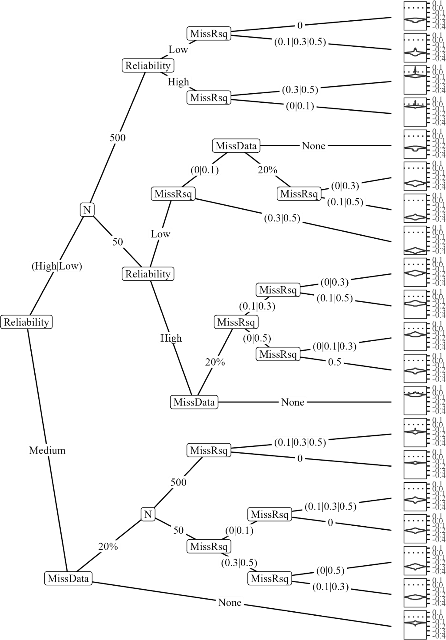
Regression Tree for Relative Bias in Slope for Observed m under EAP Scoring: TSI Not Used

Note. TSI = true score imputation; MissData = missing data; MissRsq = missingness pseudo-$R^2$.

Figure 9.

Regression Tree for Relative Bias in Slope for Mismeasured × under EAP Scoring; 10–30 Items

TSI = true score imputation; MissData = missing data; SD.x = population standard deviation (SD) of $x$.

References

- Asparouhov T, & Muthén B (2010). Plausible values for latent variables using Mplus. Unpublished. Accessed at: http://www.statmodel.com/download/Plausible.pdf.
- Beaton AE, & Gonzalez E (1995). NAEP primer. Chestnut Hill, MA: Boston College. [Google Scholar]
- Bentler PM (2017). Specificity-enhanced reliability coefficients. Psychological Methods, 22(3), 527. [DOI] [PubMed] [Google Scholar]
- Bentler PA, & Woodward JA (1980). Inequalities among lower bounds to reliability: With applications to test construction and factor analysis. Psychometrika, 45, 249–267. [Google Scholar]
- Bentler PM, & Yuan KH (1999). Structural equation modeling with small samples: Test statistics. Multivariate Behavioral Research, 34(2), 181–197. [DOI] [PubMed] [Google Scholar]
- Blackwell M, Honaker J, & King G (2017). A unified approach to measurement error and missing data: overview and applications. Sociological Methods & Research, 46(3), 303–341. [Google Scholar]
- Borsboom D, & Mellenbergh GJ (2002). True scores, latent variables, and constructs: A comment on Schmidt and Hunter. Intelligence, 30(6), 505–514. [Google Scholar]
- Breiman L (2001). Random Forests. Machine Learning, 45(1), 5–32. [Google Scholar]
- Breiman L, Friedman JH, Olshen RA, & Stone CJ (1984). Classification and Regression Trees. Chapman and Hall. [Google Scholar]
- Brennan RL (1992). Generalizability theory. Educational Measurement: Issues and Practice, 11(4), 27–34. [Google Scholar]
- Caroll RJ (1989). Covariance analysis in generalized linear measurement error models. Statistics in Medicine, 8(9), 1075–1093. [DOI] [PubMed] [Google Scholar]
- Cella D (2017). PROMIS Profiles-HUI data [Data set]. Harvard Dataverse. 10.7910/DVN/P7UKWR [DOI] [Google Scholar]
- Chalmers RP, & Adkins MC (2020). Writing effective and reliable Monte Carlo simulations with the SimDesign package. The Quantitative Methods for Psychology, 16(4), 248–280. [Google Scholar]
- Chen SK, Hou L, & Dodd BG (1998). A comparison of maximum likelihood estimation and expected a posteriori estimation in CAT using the partial credit model. Educational and Psychological Measurement, 58(4), 569–595. [Google Scholar]
- Cohen S, Kamarck T, & Mermelstein R (1983). A global measure of perceived stress. Journal of Health and Social Behavior, 385–396. [PubMed] [Google Scholar]
- Cohen S (1988). Perceived stress in a probability sample of the United States. In Spacapan S & Oskamp S (Eds.), The social psychology of health (pp. 31–67). Sage Publications, Inc. [Google Scholar]
- Cohen Y, Ben-Simon A, & Tractinsky N (1989). Computerized adaptive test of English proficiency (CATProject Report No. 6). Jerusalem, Israel: National Institute for Testing and Evaluation. [Google Scholar]
- Cole SR, Chu H, & Greenland S (2006). Multiple-imputation for measurement-error correction. International Journal of Epidemiology, 35(4), 1074–1081. [DOI] [PubMed] [Google Scholar]
- Deng L, Yang M, & Marcoulides KM (2018). Structural equation modeling with many variables: A systematic review of issues and developments. Frontiers in Psychology, 9, 580. [DOI] [PMC free article] [PubMed] [Google Scholar]
- Cronbach LJ (1951). Coefficient alpha and the internal structure of tests. Psychometrika, 16, 297–334. [Google Scholar]
- Dempster AP (1969). Elements of continuous multivariate analysis. Addison-Wesley. [Google Scholar]
- Dempster AP, Laird NM, & Rubin DB (1977). Maximum likelihood from incomplete data via the EM algorithm. Journal of the Royal Statistical Society: Series B (Methodological), 39(1), 1–22. [Google Scholar]
- Devlieger I, Mayer A, & Rosseel Y (2016). Hypothesis testing using factor score regression: A comparison of four methods. Educational and Psychological Measurement, 76(5), 741–770. [DOI] [PMC free article] [PubMed] [Google Scholar]
- Dorans NJ (2007). Linking scores from multiple health outcome instruments. Quality of Life Research, 16, 85–94. [DOI] [PubMed] [Google Scholar]
- Ellis JL (2021). A test can have multiple reliabilities. Psychometrika, 86(4), 869–876. [DOI] [PMC free article] [PubMed] [Google Scholar]
- Enders CK (2010). Applied missing data analysis. Guilford press. [Google Scholar]
- Enders CK, Keller BT, & Levy R (2018). A fully conditional specification approach to multilevel imputation of categorical and continuous variables. Psychological Methods, 23(2), 298. [DOI] [PubMed] [Google Scholar]
- Gelman A, Carlin JB, Stern HS, & Rubin DB (1995). Bayesian data analysis. Chapman and Hall/CRC. [Google Scholar]
- Ghosh-Dastidar B, & Schafer JL (2003). Multiple edit/multiple imputation for multivariate continuous data. Journal of the American Statistical Association, 98(464), 807–817. [Google Scholar]
- Goodnight JH (1979). A tutorial on the SWEEP operator. The American Statistician, 33(3), 149–158. [Google Scholar]
- Gottschall AC, West SG, & Enders CK (2012). A comparison of item-level and scale-level multiple imputation for questionnaire batteries. Multivariate Behavioral Research, 47(1), 1–25. [Google Scholar]
- Grubinger T, Zeileis A, & Pfeiffer KP (2014). evtree: Evolutionary learning of globally optimal classification and regression trees in R. Journal of Statistical Software, 61, 1–29. [Google Scholar]
- Guttman L (1945). A basis for analyzing test-retest reliability. Psychometrika, 10, 255–282. [DOI] [PubMed] [Google Scholar]
- Guo Y (2010). Multiple Imputation for Measurement Error Correction Based on a Calibration Sample [Doctoral dissertation, University of Michigan]. University of Michigan Library, Deep Blue Documents. https://deepblue.lib.umich.edu/bitstream/handle/2027.42/77676/guoy_1.pdf [Google Scholar]
- Guo Y, Little RJ, & McConnell DS (2012). On using summary statistics from an external calibration sample to correct for covariate measurement error. Epidemiology, 23(1), 165–174. [DOI] [PubMed] [Google Scholar]
- Harwell MR (1991, April). Analyzing and reporting the results of Monte Carlo studies in educational and psychological research. Paper presented at the annual meeting of the American Educational Research Association, Chicago. [Google Scholar]
- Harwell MR (1997). Analyzing the results of Monte Carlo studies in item response theory. Educational and Psychological Measurement, 57(2), 266–279. [Google Scholar]
- Harwell M, Stone CA, Hsu TC, & Kirisci L (1996). Monte Carlo studies in item response theory. Applied Psychological Measurement, 20(2), 101–125. [Google Scholar]
- Hays RD, Revicki DA, Feeny D, Fayers P, Spritzer KL, & Cella D (2016). Using linear equating to map PROMIS® global health items and the PROMIS-29 V2.0 profile measure to the health utilities index mark 3. Pharmacoeconomics, 34(10), 1015–1022. [DOI] [PMC free article] [PubMed] [Google Scholar]
- HealthMeasures. HealthMeasures Scoring Service powered by Assessment Center. Accessed October 5, 2022. https://www.assessmentcenter.net/ac_scoringse
- Honaker J, King G, & Blackwell M (2011). Amelia II: A program for missing data. Journal of Statistical Software, 45, 1–47. [Google Scholar]
- Jackson PH, & Agunwamba CC (1977). Lower bounds for the reliability of the total score on a test composed of non-homogeneous items: I: Algebraic lower bounds. Psychometrika, 42, 567–578. [Google Scholar]
- Jorgensen TD, Pornprasertmanit S, Schoemann AM, & Rosseel Y (2021). semTools: Useful tools for structural equation modeling. R package version 0.5–5. Retrieved from https://CRAN.R-project.org/package=semTools [Google Scholar]
- Jurek AM, Maldonado G, Greenland S, & Church TR (2006). Exposure-measurement error is frequently ignored when interpreting epidemiologic study results. European Journal of Epidemiology, 21(12), 871–876. [DOI] [PubMed] [Google Scholar]
- Kelley TL (1927). Interpretation of educational measurements. World Book Co. [Google Scholar]
- Kim JK, & Nicewander WA (1993). Ability estimation for conventional tests. Psychometrika, 58(4), 587–599. [Google Scholar]
- Kupst MJ, Butt Z, Stoney CM, Griffith JW, Salsman JM, Folkman S, & Cella D (2015). Assessment of stress and self-efficacy for the NIH Toolbox for Neurological and Behavioral Function. Anxiety, Stress, & Coping, 28(5), 531–544. [DOI] [PMC free article] [PubMed] [Google Scholar]
- Little RJ, and Rubin DB (2014). Statistical analysis with missing data. John Wiley & Sons. [Google Scholar]
- Lord FM (1983). Unbiased estimators of ability parameters, of their variance, and of their parallel-forms reliability. Psychometrika, 48(2), 233–245. [Google Scholar]
- Lord FM (1986). Maximum likelihood and Bayesian parameter estimation in item response theory. Journal of Educational Measurement, 23(2), 157–162. [Google Scholar]
- Mansolf, 2022. A True Score Imputation Method to Account for Psychometric Measurement Error. OSF repository. Retrieved from https://osf.io/83ghx/ [DOI] [PMC free article] [PubMed] [Google Scholar]
- Masters GN, Lokan J, Doig BA, Khoo ST, Lindsey J, Robinson L, & Zammit S (1990). Profiles of learning: The Basic Skills Testing Program in New South Wales, 1989. Hawthorn, Australia: Australian Council for Educational Research. [Google Scholar]
- Mazza GL, Enders CK, & Ruehlman LS (2015). Addressing item-level missing data: A comparison of proration and full information maximum likelihood estimation. Multivariate Behavioral Research, 50(5), 504–519. [DOI] [PMC free article] [PubMed] [Google Scholar]
- McDonald RP (1999). Test theory: A unified approach. Mahwah, NJ: Erlbaum. [Google Scholar]
- McKelvey RD, & Zavoina W (1975). A statistical model for the analysis of ordinal level dependent variables. Journal of Mathematical Sociology, 4(1), 103–120. [Google Scholar]
- Mislevy RJ (1991). Randomization-based inference about latent variables from complex samples. Psychometrika, 56, 177–196. [Google Scholar]
- Mislevy RJ, Beaton AE, Kaplan B, & Sheehan KM (1992). Estimating population characteristics from sparse matrix samples of item responses. Journal of Educational Measurement, 29(2), 133–161. [Google Scholar]
- Muthén LK, & Muthén BO (1998–2017). Mplus User’s Guide. Eighth Edition. Muthén & Muthén. [Google Scholar]
- Nunnally JC (1978). Psychometric theory (2nd ed.). New York: McGraw-Hill. [Google Scholar]
- R Core Team (2022). R: A language and environment for statistical computing. R Foundation for Statistical Computing. URL https://www.R-project.org/. [Google Scholar]
- Revelle W, & Zinbarg RE (2009). Coefficients alpha, beta, omega, and the glb: Comments on Sijtsma. Psychometrika, 74(1), 145–154. [Google Scholar]
- Robitzsch A, & Grund S (2022). miceadds: Some Additional Multiple Imputation Functions, Especially for ‘mice’. R package version 3.14–3. https://CRAN.R-project.org/package=miceadds [Google Scholar]
- Rubin DB (1987). Multiple imputation for nonresponse in surveys (Vol. 81). John Wiley & Sons. [Google Scholar]
- Samejima F (1968). Estimation of latent ability using a response pattern of graded scores 1. ETS Research Bulletin Series, 1968(1), i–169. [Google Scholar]
- Schafer Joseph L. Analysis of incomplete multivariate data. Chapman and Hall/CRC, 1997. [Google Scholar]
- Schmidt FL & Hunter JE (1999). Theory testing and measurement error. Intelligence, 27(3), 183–198. [Google Scholar]
- Sijtsma K, & Pfadt JM (2021). Rejoinder: The future of reliability. Psychometrika, 86(4), 887–892. [DOI] [PMC free article] [PubMed] [Google Scholar]
- Spearman C (1904). The proof and measurement of association between two things. American Journal of Psychology, 15, 72–101. [PubMed] [Google Scholar]
- Spearman C (1910). Correlation calculated from faulty data. British Journal of Psychology, 3, 271–295. [Google Scholar]
- Strobl C, Malley J, & Tutz G (2009). An introduction to recursive partitioning: rationale, application, and characteristics of classification and regression trees, bagging, and random forests. Psychological Methods, 14(4), 323. [DOI] [PMC free article] [PubMed] [Google Scholar]
- Van Buuren S & Groothuis-Oudshoorn K (2011). mice: Multivariate Imputation by Chained Equations in R. Journal of Statistical Software, 45(3), 1–67. doi: 10.18637/jss.v045.i03. [DOI] [Google Scholar]
- Van Buuren S & Oudshoorn K (1999). Flexible multivariate imputation by MICE. TNO Prevention and Health. [Google Scholar]
- Wandall J (2011). National tests in Denmark–CAT as a pedagogic tool. Journal of Applied Testing Technology, 12(1). [Google Scholar]
- Wang T, & Vispoel WP (1998). Properties of ability estimation methods in computerized adaptive testing. Journal of Educational Measurement, 35(2), 109–135. [Google Scholar]
- Winkler WE (2003), “A Contingency-Table Model for Imputing Data Satisfying Analytic Constraints,” technical report, Statistical Research Division, U.S. Bureau of the Census. [Google Scholar]
- Woodhouse B, & Jackson PH (1977). Lower bounds for the reliability of the total score on a test composed of non-homogeneous items: II: A search procedure to locate the greatest lower bound. Psychometrika, 42, 579–591. [Google Scholar]
- Wright MN & Ziegler A (2017). ranger: A fast implementation of random forests for high dimensional data in C++ and R. Journal of Statistical Software, 77(1), 1–17. doi: 10.18637/jss.v077.i01 [DOI] [Google Scholar]
Associated Data
This section collects any data citations, data availability statements, or supplementary materials included in this article.