

Abstract
Within the aortic valve (AV) leaflet exists a population of interstitial cells (AVICs) that maintain the constituent tissues by extracellular matrix (ECM) secretion, degradation, and remodeling. AVICs can transition from a quiescent, fibroblast-like phenotype to an activated, myofibroblast phenotype in response to growth or disease. AVIC dysfunction has been implicated in AV disease processes, yet our understanding of AVIC function remains quite limited. A major characteristic of the AVIC phenotype is its contractile state, driven by contractile forces generated by the underlying stress fibers (SF). However, direct assessment of the AVIC SF contractile state and structure within physiologically mimicking three-dimensional environments remains technically challenging, as the size of single SFs are below the resolution of light microscopy. Therefore, in the present study, we developed a three-dimensional (3D) computational approach of AVICs embedded in 3D hydrogels to estimate their SF local orientations and contractile forces. One challenge with this approach is that AVICs will remodel the hydrogel, so that the gel moduli will vary spatially. We thus utilized our previous approach (Khang et al. 2023, “Estimation of Aortic Valve Interstitial Cell-Induced 3D Remodeling of Poly (Ethylene Glycol) Hydrogel Environments Using an Inverse Finite Element Approach,” Acta Biomater., 160, pp. 123–133) to define local hydrogel mechanical properties. The AVIC SF model incorporated known cytosol and nucleus mechanical behaviors, with the cell membrane assumed to be perfectly bonded to the surrounding hydrogel. The AVIC SFs were first modeled as locally unidirectional hyperelastic fibers with a contractile force component. An adjoint-based inverse modeling approach was developed to estimate local SF orientation and contractile force. Substantial heterogeneity in SF force and orientations were observed, with the greatest levels of SF alignment and contractile forces occurring in AVIC protrusions. The addition of a dispersed SF orientation to the modeling approach did not substantially alter these findings. To the best of our knowledge, we report the first fully 3D computational contractile cell models which can predict locally varying stress fiber orientation and contractile force levels.
Keywords: aortic valve interstitial cell, cell mechanics modeling, 3D traction force microscopy, computational modeling, adjoint method
1 Introduction
The aortic valve (AV), positioned between the aorta and the left ventricle, ensures unidirectional flow of oxygenated blood from the heart to the body. This deceptively simple function requires a careful interplay of cellular, tissue, and organ-level structures to ensure usually flawless function over a lifetime. The AV consists of three leaflets (often called cusps due to their shape), composed of three histologically distinct layers in the majority of the leaflet. All layers contain AV interstitial cells (AVICs), which are fibroblast-like cells that maintain the leaflet tissue structures. This role is accomplished by the AVICs through ECM secretion, degradation, and remodeling [1,2]. AVICs can also transition from a quiescent, fibroblast-like phenotype to an activated, myofibroblast phenotype in response to growth [3] or disease [1,2,4–6]. The activated AVIC phenotype is characterized by increases in proliferation, ECM remodeling and deposition, increased expression of α smooth muscle actin (α-SMA), and enhanced cellular contractility induced by augmented contraction of the stress fibers (SFs) (Fig. 1) [1,2,4,5]. Pathological persistence of the myofibroblast phenotype has been implicated in excessive ECM deposition, eventually leading to fibrosis or stiffening of the valve, resulting in AV stenosis.
Fig. 1.
![AVIC subcellular structures. (a) Superimposed image of an AVIC within a three-dimensional (3D) PEG hydrogel environment generated by combining images of (b) filamentous actin, (c) α-SMA, and (d) the nucleus. The images are maximum intensity projections of a 3D image set in the x-z plane. (Images taken from Khang et al. [7]).](https://cdn.ncbi.nlm.nih.gov/pmc/blobs/f504/10680985/7907fb690a86/bio-23-1085_121005_g001.jpg)
AVIC subcellular structures. (a) Superimposed image of an AVIC within a three-dimensional (3D) PEG hydrogel environment generated by combining images of (b) filamentous actin, (c) α-SMA, and (d) the nucleus. The images are maximum intensity projections of a 3D image set in the x-z plane. (Images taken from Khang et al. [7]).
Local variations in SF expression and orientation affect AVIC mechanical function [1,2,4–6] and can serve as a biophysical marker of AVIC activation levels and phenotypic state [1,2,4–6,8,9]. This is supported by ex situ studies of diseased valves which showed that AVIC activation levels, as assessed by expression levels of α-SMA, are elevated in diseases such as calcific AV disease [10,11], bicuspid AV disease [12,13], and fibrotic cardiac disease [14]. Thus, it is clear that SFs play a critical role in AVIC function, yet our knowledge of their pathophysiological function remains quite limited. As a critical part of cellular function, SFs are dynamic structures that exist in a diffuse or discrete form in response to mechanical and pathological cues. Previous studies have largely utilized two-dimensional (2D) in vitro techniques [8,9,15–18] or explanted native AV tissues [17–20] to assess AVIC contractile behaviors toward understanding underlying SF properties. For example, AVICs in 2D in vitro studies increase their contractility through the formation of discrete and densely packed SF bundles when seeded on stiff substrates [8,9]. However, imparting realistic 3D cues continues to be a challenge in 2D in vitro studies. As with most cells, AVICs exist in a complex 3D micro-environment and respond to physical queues, such as cyclic stretch at the tissue level [21,22]. However, studies within the native 3D environment are also quite challenging. Specifically, direct imaging of AVIC subcellular structures within native tissues is not possible due to the dense nature of AV tissues. Another challenge in understanding AVIC SF behaviors is that the feature size of single SFs are well below what can be resolved using light microscopy. Although super-resolution microscopy can resolve AVIC SFs at higher resolutions, they are commonly depth limited and cannot obtain images in the ranges required to completely capture AVIC SFs within 3D environments (∼140 μm deep).
To begin to address these limitations, hydrogels have been used as 3D biomimicking environments that allow for direct imaging of AVIC structures [7,23–28]. Hydrogel materials mimic many of the key properties of native tissues such as incorporation of enzymatically degradable peptide cross-links, adhesive protein sequences, and allowing for full 3D culture and assessment [29]. Hydrogel environments also allow for 3D assessment of cell contractile behaviors through the use of three-dimensional traction force microscopy, which measures the geometry and deformation induced by biological cells [7,24,30–38]. From these measurements, the traction forces produced by the cell can be computed with prior knowledge of the material properties.
The use of hydrogels in the study of cell mechanics is not straightforward. For instance, hydrogels can be affected by cell-induced local remodeling, which can impart degradation via enzymatic activity or stiffening by ECM deposition. Traction force microscopy, widely used in cell mechanics, requires precise knowledge of the local gel mechanical behaviors for extraction of the underlying cellular forces [33]. Previous approaches have largely assumed that macroscopic-level hydrogel mechanical properties can be treated as homogeneous and remain unmodified by the cellular activity. However, both of these assumptions are likely not realistic in enzyme-degradable three-dimensional hydrogel cultures. Moreover, in situ mechanical properties of hydrogel materials are challenging to measure using extant experimental methods. To address these experimental shortcomings, we recently developed an inverse finite-element modeling approach to estimate the local hydrogel mechanical properties near an embedded AVIC [39]. In summary, this approach produced a spatially varying hydrogel modulus field that minimized the error between the experimentally measured and simulated hydrogel deformations produced by a contracting AVIC. It was determined that AVICs locally degrade (likely through enzymatic secretion) as well as stiffen the hydrogel through collagen deposition.
In the present work, we developed a fully three-dimensional continuum computational model of a contracting AVIC embedded within a hydrogel environment. Our modeling approach accounted for spatially varying hydrogel mechanical properties to determine the AVIC SF architecture and contractile forces. To inform our model on the nucleus and cytosol behaviors, we used values from our previous and other related studies [40–43]. Moreover, we utilized our previous continuum modeling approach of AVIC mechanics (seeded on 2D surfaces) that assumed that AVIC SFs have an intrinsic force generating capability per unit mass, with the local effective force being a function of the SF orientation and mass fraction [40,41]. We then developed two model forms of the local SF: a single fiber and a dispersed fiber orientation. Use of these two approaches was used to gain insights into the effects of local SF structures on predicted effective SF behaviors. For instance, the single fiber contraction model can be used to model the effective behavior of contracting AVICs, while still obtaining crucial knowledge of SF orientation and contraction levels. The fiber dispersion model can be used to gain higher fidelity information in cellular regions in which the SF orientation may be amorphous (e.g., cellular midsection). This approach allowed us to determine the effective AVIC contractile behaviors in a computationally tractable framework.
2 Methods
2.1 Summary of Three-Dimensional Traction Force Microscopy.
The experimental methods used in the current study have been described in detail in previous studies [39,7,24,35]. Briefly, AVICs were extracted from porcine hearts obtained from a local abattoir (Harvest House Farms, Johnson City, TX) using published methods [44]. Three-dimensional traction force microscopy measurements were performed by staining AVICs with CellBriteTM Red (Biotum, Hayward, CA) before encapsulation within poly (ethylene glycol) (PEG) hydrogels comprised of 8-arm 40-kDa norbornene functionalized PEG molecules (JenKem, Beijing, China), adhesive peptide sequences (CRGDS, Bachem), and matrix metalloproteinase degradable cross-linking peptides (Bachem, Bubendorf, Switzerland) [25,45]. Additionally, 0.5-μm-diameter yellow-green fluorescent microspheres (Polysciences, Warrington, PA) were added within the PEG hydrogel as fiducial markers to track AVIC-induced displacements. Three-dimensional z-stack image sets containing single AVICs and surrounding fluorescent microspheres within the PEG hydrogel were obtained for each AVIC: (1) after 40 min of incubation within Tyrode's Salt Solution (basal contraction present) and then (2) after 40 min of incubation within Cytochalasin D (relaxed condition). The spatial positions of the imaged fluorescent microspheres were tracked using our open-source software FM-Track [35]. In addition, FM-Track generated surface mesh representations of the imaged AVIC geometries.
2.2 Overall Modeling Approach.
We defined the simulation domain Ω as consisting of the hydrogel and AVIC subdomains (Fig. 2), defined as follows
| (1) |
Fig. 2.
![Schematic illustrating our integrated modeling approach consisting of the hydrogel domain model and the single SF and dispersed SF AVIC models. The modeling approach is defined over a single domain (top) representing the TFM experiment and separated into the gel and AVIC subdomains which share the AVIC membrane boundary. In the hydrogel domain, we used previously defined detailed regional mechanical properties [39]. We were then able to determine AVIC stress fiber forces and orientations in either SF model.](https://cdn.ncbi.nlm.nih.gov/pmc/blobs/f504/10680985/04a4fadc374f/bio-23-1085_121005_g002.jpg)
Schematic illustrating our integrated modeling approach consisting of the hydrogel domain model and the single SF and dispersed SF AVIC models. The modeling approach is defined over a single domain (top) representing the TFM experiment and separated into the gel and AVIC subdomains which share the AVIC membrane boundary. In the hydrogel domain, we used previously defined detailed regional mechanical properties [39]. We were then able to determine AVIC stress fiber forces and orientations in either SF model.
where Ωcyto + sf, Ωnuc, and Ωgel represent the AVIC combined cytoplasm and SF, nucleus, and hydrogel domains, respectively. We assumed that there were no inertial or body forces present, so that the conservation of linear momentum yields
| (2) |
Following [39,40,41], both the AVIC and hydrogel subdomains were modeled as hyperelastic materials with the following strain energy function (Ψ)
| (3) |
using the same subscript definition as in Eq. (1). Details of how each Ψ component was formulated is given in Secs. 2.3 and 2.4.
2.3 The Hydrogel Subdomain.
Accurate estimation of the AVIC tractions and SF force system requires detailed knowledge of spatial distribution of the hydrogel mechanical behaviors. This is particularly important when using matrix metalloproteinase-degradable hydrogels, which are subject to modification by AVIC-induced enzymatic degradation and ECM protein deposition. Not accounting for cell-induced modifications in three-dimensional environments can lead to large errors in computed cellular tractions [33]. We have recently developed an inverse finite-element modeling approach to accurately estimate the local hydrogel mechanical properties surrounding an embedded AVIC [39]. Utilization of the resultant remodeled hydrogel modulus map allowed us to develop an accurate inverse model of embedded AVIC SF behaviors.
Details of the methods and findings of the hydrogel model have been presented in [39]. In brief, the hydrogel was modeled as a neo-Hookean solid, with a modulus scaling parameter α(x0) that varied as a function of position x0. The resulting hydrogel material model was
| (4) |
where α(x0) can fall into one of the following ranges
| (5) |
and and are material constants, is the first invariant of the isochoric part of the Right Cauchy Green deformation tensor ( = J−2/3C, C = FT F, F is the deformation gradient tensor, and J = det(F)). This form is consistent with the small strain limit in which approaches one half the shear modulus of the hydrogel μgel and approaches one half the first Lamé parameter λgel. A value of α(x0) = 1 corresponded to the unmodified = 54 Pa. Thus, at each nodal position x0, the effective neo-Hookean model modulus is α(x0) . Next, we assumed that at a sufficient distance from the AVIC (i.e., near the problem domain boundary), the hydrogel remained unmodified so that α(x0) = 1. The local values of α(x0) within the domain of the hydrogel were estimated by solving an inverse problem which minimized the error between the experimental and simulated AVIC-induced hydrogel deformations. Specifically, we minimized the error between the Right Cauchy Green deformation tensors of the simulation and the experimental results at the nodes of the finite element (FE) mesh. The end point of this approach was a detailed effective modulus map of the hydrogel subdomain defined at each FE node of the hydrogel mesh. An example of the hydrogel model with spatial varying moduli clearly shows regions of both degradation and stiffening in the local vicinity of the AVIC (Fig. 3). The hydrogel materials near AVIC protrusions were stiffened to approximately two times the pristine hydrogel stiffness μgel (∼200 Pa versus 108 Pa). Degraded hydrogel regions were more uniformly distributed around the AVIC midsection and were degraded to as low as ∼60 Pa. These results underscore the need for determining accurate hydrogel mechanical properties.
Fig. 3.
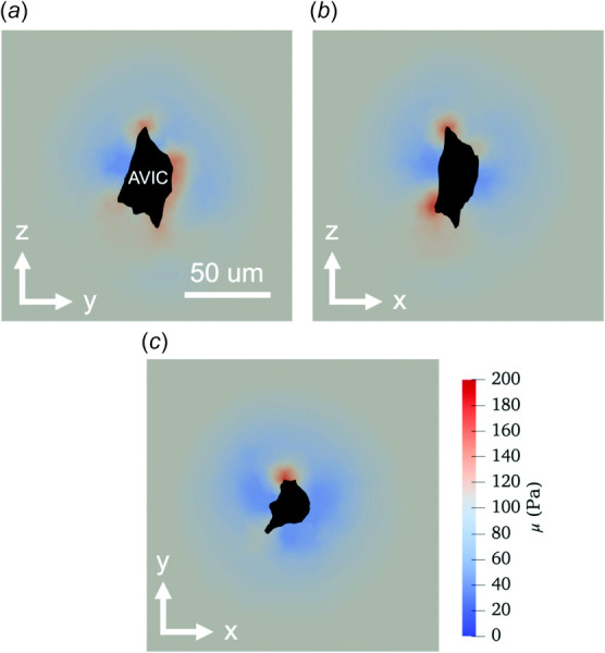
Two-dimensional cross sections of the inverse hydrogel modeling results in the (a) Y–Z, (b) X–Z, and (c) X–Y planes depicting degraded (< 108 Pa, blue), stiffened (>108 Pa, red), and unmodified (108 Pa, gray) regions within the hydrogel domain near the AVIC geometry (black). (For interpretation of the references to color in this figure legend, the reader is referred to the web version of this article.)
2.4 The Aortic Valve Interstitial Cell Subdomain
2.4.1 The Cytosol and Nucleus.
Following our previous approaches [40,41], we idealized the AVIC as consisting of cytosol, nucleus, and SFs that act as a solid mixture that deforms together. For the cytoplasm itself (i.e., without the SFs), we utilized an isotropic neo-Hookean hyperelastic material model using a nearly incompressible formulation
| (6) |
where = in the small strain limit, μcyto is the shear modulus of the cytoplasm, = in the small strain limit, and λcyto is Lamé's first parameter. The second Piola–Kirchoff stress, Scyto, was then determined using
| (7) |
Next, we idealized the AVIC nucleus as a general ellipsoid, with the average nuclear volume, aspect ratio, centroid, and orientation determined from extant fluorescent images of AVICs embedded within 3D hydrogels similar to those shown in Fig. 1. In brief, we found that on average, the AVIC volume to nuclear volume ratio was approximately 4.5 to 1, AVIC nuclear aspect ratio was 4:2.5:1, and that the AVIC nucleus shared the same centroid and orientation as the AVIC body. This information allowed for the generation of nuclear geometries for the simulations, despite the nuclear geometries not being imaged/captured during the live 3D TFM experiments. We note that the mechanical contributions of the nucleus are likely small but felt it added a degree of realism to the present models. The AVIC nucleus was assumed to be a neo-Hookean solid with the following strain energy density function
| (8) |
where = in the small strain limit, μnuc is the shear modulus of the nucleus, = in the small strain limit, and λnuc is Lamé's first parameter. Snuc was then determined using
| (9) |
2.4.2 The Aortic Valve Interstitial Cell Single Fiber Contraction Model.
SFs were modeled within the cytoplasm domain Ωcyto + sf and continuity of displacement is assumed so that
| (10) |
As in [40,41], we split the SF response into a passive and active component. For the passive component, the SF strain energy function (Ψsf) was [46]
| (11) |
where μsf is the SF modulus and ϕsf is the SF mass fraction. Alternatively, ϕsf can be interpreted as the SF expression level. The resulting stress tensor Sp can be computed using [47]
| (12) |
where
| (13) |
and
| (14) |
where m0 = m0(θ, ϕ) is the local SF fiber orientation vector expressed using (θ, ϕ) spherical coordinates in the referential configuration (Fig. 4(a)). The resulting complete form of Sp is
| (15) |
Fig. 4.
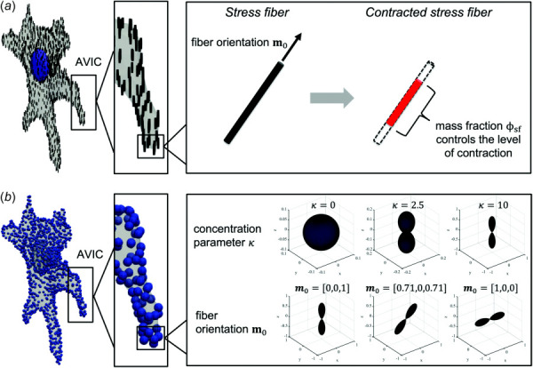
Schematic illustrating parameters estimated from the two inverse cell modeling approaches. (a) The parameters estimated from the single fiber contraction model include the SF orientation m0 and the SF mass fraction ϕsf, which controls the level of SF contraction. (b) The parameters estimated from the fiber dispersion model include the von Mises orientation distribution function concentration parameter κ, fiber orientation m0, and the SF mass fraction ϕsf (not shown in schema).
Here, a Heaviside step function H was introduced to ensure that passive stretch only arises from fiber extension and not compression. Specifically,
| (16) |
Next, the SF active stress Sa was defined as
| (17) |
where fsf is the SF contractile force per unit fiber mass and ϕsf is the SF mass fraction. This results in a total SF stress Ssf
| (18) |
2.4.3 The Aortic Valve Interstitial Cell Stress Fiber Dispersion Model.
We developed an extended mathematical formulation for the SF phase utilizing fiber dispersion as we observed that SFs can form dispersed networks (Fig. 1). The formulation of this approach is essentially the same as the single fiber contraction model, only now the SF can have a local 3D dispersion architecture. To implement this, we assumed that SF stresses were influenced by the local orientation of SFs which can be described using a 3D von Mises distribution
| (19) |
where Γ(m0, n) is a von Mises orientation distribution function with preferred direction m0 for any given orientation n. This results in the following form
| (20) |
where (κ ∗ cos(cos−1(m0 · n))) sinθ dθ dϕ and both Sp and Sa are functions of θ and ϕ through m0 (see Eqs. (15) and (17)). Here, κ is the concentration parameter, n is a given fiber orientation, and A is a scaling constant chosen such that sinθ dθ dϕ = 1 (Fig. 4(b)). Note that κ is inversely proportional to dispersion width, with a value of κ = 0 denoting a uniform distribution, whereas a high value of κ causes the distribution to become highly concentrated about m0 (Fig. 4(b)). Thus, as κ → ∞, this model will approach the single fiber contraction model discussed in Sec. 2.4.2.
2.5 Numerical Solutions of the Combined Hydrogel and Aortic Valve Interstitial Cell Models.
All simulations were performed in FEniCS, which is an open-source, Python-based finite-element solver available online2. The model parameters used in this study and how their values were determined are detailed in Table 1.
Table 1.
AVIC forward model parameters
| Parameter | Description | Value | Source |
|---|---|---|---|
| Φ sf | Stress fiber mass fraction | — | Backed out by model |
| m 0 | Stress fiber initial orientation | — | Backed out by model |
| κ | Von Mises distribution concentration parameter | — | Backed out by model |
| μ gel | Shear modulus of gel | Varying | Ref. [39] |
| μ cyto | Shear modulus of cytoplasm | 750 Pa | Ref. [40,41] |
| μ nuc | Shear modulus of nucleus | 7500 Pa | Ref. [40,41] |
| μ sf | Shear modulus of stress fiber | 390 Pa | Ref. [40,41] |
| ν gel,cyto,nuc | Lamé's first parameter | Identity | |
| λ gel,cyto,nuc | Poisson ratio | 0.49 | Assumed Ref. [40,41] |
| f sf | Stress fiber contractile stress per unit fiber | 1000 Pa | Ref. [40,41] |
2.5.1 Note on the Forward Finite Element Model.
We used the open-source software Gmsh [48] to generate 3D FE meshes of the AVIC embedded within the hydrogel mesh domain. No displacement boundary conditions were applied to the outer boundary of the hydrogel domain. The inner boundary of the hydrogel shared nodes with the boundary of the AVIC and was assumed to be perfectly bonded, so that their displacements were equivalent at the subdomain interface. Similarly, the inner boundary of the AVIC cytoplasm shared nodes with the boundary of the nucleus, so that their displacements were equivalent at the interface. The final problem mesh consisted of approximately 50,000 linear tetrahedral elements. Mesh convergence analysis was performed in our prior study [39], which showed that using more than 50,000 linear tetrahedral elements did not result in significantly different simulation results. The double integrals in Eq. (20) were computed numerically using Gaussian quadrature to ensure efficient computation time. Both forward models were ran by initially prescribing a SF contraction strength fsf = 1 kPa.
2.5.2 Adjoint-Based Inverse Modeling Approach.
Following similar methods developed for the inverse hydrogel model [39], an adjoint-based inverse computational method was used. We used dolfin-adjoint3 to automatically derive the discrete adjoint and tangent linear models from a forward computational model in FEniCS [49]. This model was employed to estimate the spatially varying parameters ϕsf, m0, and κ within the AVIC cytosol (i.e., Ωcyto + sf) by minimizing the error in the hydrogel deformation field between the experiment and simulation. This was done by minimizing the following objective function f for the 3D AVIC single fiber contraction model
| (21) |
where ξ = Csim − Cexp, Csim, and Cexp are the Right Cauchy Green deformation tensors for the hydrogel simulation and experimental results, respectively, : is the scalar tensor product operator, and β and γ are regularization parameters. Similarly, the objective function for the 3D AVIC fiber dispersion model was formulated as
| (22) |
where δ is an additional regularization parameter. The second and third terms of Eqs. (21) and (22) penalize the gradient of the SF mass fraction (ϕsf) and the gradient of the SF initial orientation (m0), respectively. The fourth term of Eq. (22) penalizes the gradient of the von Mises distribution concentration parameter κ. These terms effectively enforce the smoothness of the scalar field ϕsf, the vector field m0, and the scalar field κ. The term ∇ϕsf ∇ϕsf can be explicitly expressed as follows
| (23) |
whereas the term ∇m0:∇m0 is expressed as
| (24) |
and the term ∇κ ∇κ is expressed as
| (25) |
For both the single fiber contraction and fiber dispersion models, the optimal value for the regularization parameters were determined using the same approach in the hydrogel model [39] that utilized the “L-curve” method [50]. The regularization parameter value was determined as to prioritize the minimization of the error between the simulated and experimental deformations (first term of Eqs. (21) and (22)) while still ensuring that the estimated parameter fields of ϕsf, m0, and κ were smooth.
The AVIC inverse model pipeline is shown conceptually in Fig. 5. The initial conditions of the single fiber contraction model consisted of uniformly oriented SFs in the global z-coordinate direction (m0 = [0, 0, 1]) and uniform stress fiber mass fraction (ϕsf = 1). The initial conditions for the fiber dispersion model were the same as the single fiber contraction model with the addition of uniform von Mises distribution concentration parameter (κ = 1). The adjoint-based inverse model was run until the function tolerance was less than 1 × 10⁻⁸, resulting in the optimal values for ϕsf, m0, and κ. The remaining simulation parameters used in this study are included in Table 2. The range for the parameter ϕsf was [0,1] whose limits represent no SF expression and maximum SF expression. The range for the parameter κ was set to [0,100] whose limits represent a completely isotropic fiber distribution to a completely aligned fiber distribution. It is important to note that no information regarding SF orientation or concentration was derived from experimentally imaged AVICs.
Fig. 5.
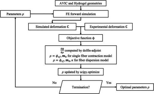
Flow chart depicting the inverse modeling approach. Discretized finite-element meshes of the AVIC and hydrogel domains are used to run the forward model. Then, the objective function, defined as the error between the simulated and experimental deformation field, is computed. Next, the gradient of the objective function with respect to all values of ρ(x0) is computed using dolfin-adjoint. Here, ρ(x0) represents the spatially varying parameters ϕsf and m0 for the single fiber contraction model and ϕsf, m0, and κ for the fiber dispersion model. Then, an updated parameter set for ρ was obtained using the L-BFGS-B algorithm in scipy.optimize, which results in a decrease to the objective function. This process is iterated until a termination criterion is met.
Table 2.
AVIC inverse model parameters
| Parameter | Description | Value |
|---|---|---|
| F tol | Function tolerance for termination | 1 × 10⁻⁸ |
| Mesh density | Number of tetrahedral elements in the finite-element mesh | 50,000 |
| Degree | Degree of finite elements | 1 |
| Scipy minimize algorithm | Algorithm used for minimization | L-BFGS-B |
| Max iterations | Maximum iterations allowed for minimization algorithm | 5000 |
| β | Regularization scaling parameter for ϕsf | 0.001 |
| γ | Regularization scaling parameter for m0 | 0.001 |
| δ | Regularization scaling parameter for κ | 0.001 |
| ϕsf [lb,ub] | Lower and upper bounds for ϕsf | [0,1] |
| m0 [lb,ub] | Lower and upper bounds for m0 | [−1,1] |
| κ [lb,ub] | Lower and upper bounds for κ | [0,100] |
2.5.3 Inverse Model Results Post-Processing.
We determined the SF contractile force using
| (26) |
where fsf is the contractile stress per unit SF determined from previous studies [40,41], ϕsf is the fiber mass fraction determined from the inverse model, and Asf is the cross-sectional area of the SFs, which were assumed to be cylindrical with a radius of 3.5 nm [51]. The computation of SF contractile force allowed for the assessment of total AVIC contractile force which was computed using
| (27) |
3 Results
3.1 Overall Inverse Model Performance.
Overall, the converged solutions featured smooth SF orientation and contractile force fields. The mean and standard deviation of the error (ξ: ξ) between the target and simulation at the hydrogel mesh nodal locations was 0.004 ± 0.01 for both cell models. We note that the single fiber contraction model and the fiber dispersion model produced virtually the same level of error. Extensive model validation for our adjoint-based inverse model was performed in our prior article [1]. In brief, test problems were created with a known parameter field, and we used our inverse modeling approach to estimate these parameters beginning from an initial guess of a homogeneous parameter field. We demonstrate excellent estimation of the parameter fields with and without the presence of experimental noise. In addition, validation specific to the cell model was performed, and the results showed good agreement between ground truth and estimated datasets (see Appendix).
3.2 Single Fiber Contraction Model.
The single direction SF model predicted that SFs are both highly aligned locally and highly contractile at AVIC protrusions (Fig. 6). Moreover, the model predicted that the greatest SF contractile forces were localized at the tip of the AVIC protrusion (Fig. 6(a)) with an average SF force of 10.02 ± 5.06 fN, which corresponded with a ϕsf value of 0.260 ± 0.132 (Table 3). Furthermore, the model predicted that the AVIC midsection (Fig. 6(c)) contained less contractile SFs relative to the protrusions, with an average contractile force of 5.93 ± 4.82 fN corresponding with a ϕsf value of 0.154 ± 0.125 (Table 3).
Fig. 6.
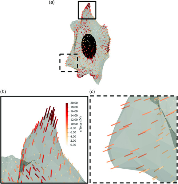
Representative inverse modeling results for the single fiber contraction model. (a) A simulated AVIC with local SF direction denoted by lines. The color scale indicates the SF force levels. (b) A close-up view of an AVIC protrusion demarcated by the solid square in panel (a). (c)A close-up view of the AVIC midsection demarcated by the dashed square in panel (a). The SF force levels are greater at AVIC protrusions than the AVIC midsection.
Table 3.
Summarized results for cell models
| Model | Location | Parameter | Mean ± STD |
|---|---|---|---|
| Single fiber contraction | Midsection | Φ sf | 0.154 ± 0.125 |
| SF force | 5.93 ± 4.82 fN | ||
| Protrusion | Φ sf | 0.260 ± 0.132 | |
| SF force | 10.02 ± 5.06 fN | ||
| Fiber dispersion | Midsection | Φsf | 0.543 ± 0.164 |
| SF force | 20.88 ± 6.30 fN | ||
| κ | 2.07 ± 0.20 | ||
| Protrusion | Φ sf | 0.619 ± 0.107 | |
| SF force | 23.82 ± 4.10 fN | ||
| κ | 2.22 ± 0.23 |
3.3 Fiber Dispersion Model.
The fiber dispersion model predicted similar fiber orientations at AVIC protrusions compared to the single fiber contraction model (Figs. 6(b) and 7(b)). However, the SF orientation at the midsection of the cell appeared to be orthogonal to the SF orientation predicted by the single fiber contraction model (Figs. 6(c) and 7(c)). Moreover, the model predicted that SFs were more highly aligned at AVIC protrusions (Fig. 7(b)) with a mean κ value of 2.22 ± 0.23 (Table 3) compared to the AVIC midsection (Fig. 7(c)) which had a mean κ value of 2.07 ± 0.20 (Table 3). In addition, the model predicted that SF contractile forces were greater at AVIC protrusions (23.82 ± 4.10 fN, Table 3) than at the AVIC midsection (20.88 ± 6.30 fN, Table 3).
Fig. 7.
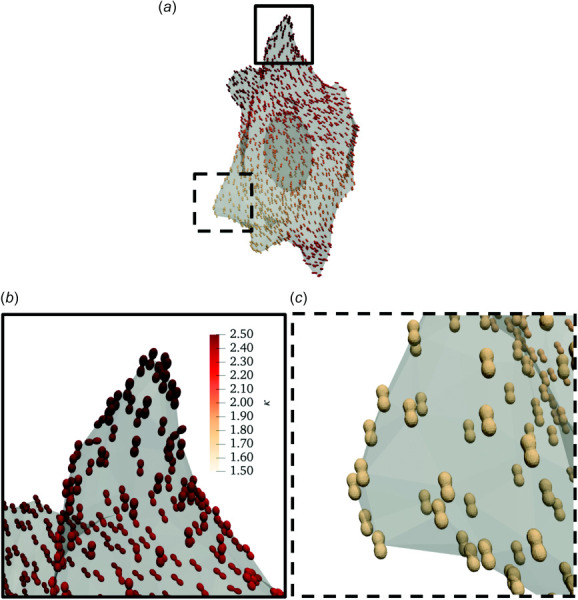
Representative inverse modeling results for the fiber dispersion model. (a) A simulated AVIC with local SF direction and concentration denoted by von Mises distributions represented as local glyphs. The color scale indicates the von Mises distribution concentration parameter κ. (b) A close-up view of an AVIC protrusion demarcated by the solid square in panel (a). (c) A close-up view of the AVIC midsection demarcated by the dashed square in panel (a). The SF concentration parameters are greater at AVIC protrusions than the AVIC midsection, indicating a greater degree of SF alignment.
4 Discussion
4.1 Major Findings
4.1.1 Stress Fiber Orientation and Contractility in Aortic Valve Interstitial Cell Protrusions.
The simulation results show that both SF orientation and contractile force were highly spatially uniform within the AVIC protrusions (Figs. 6 and 7). These results are consistent with cell images using immunostaining that depict regions of aligned SFs and abundant expression in AVIC protrusions (Fig. 1). Moreover, the simulation results are consistent with experimental findings previously reported in [15] which showed that AVIC protrusions deform in a uniform, piston-like manner which is indicative of an underlying, highly aligned SF architecture. This is in line with broadly accepted notions of cellular protrusions being highly contractile structures that allow for cell migration and mechanosensing [52].
4.1.2 Stress Fiber Orientation and Contractility at the Aortic Valve Interstitial Cell Midsection.
The SF orientation at the midsection of the AVIC varied between the single fiber contraction model (Fig. 6(c)) and the fiber dispersion model (Fig. 7(c)). The fiber orientations appeared nearly orthogonal between the two models in these regions. We hypothesize that this is partially due to the low levels of contractile force at the AVIC midsection. Specifically, because the SFs at the midsection are not very contractile relative to the protrusions, their orientation is not as critical nor as meaningful as the SF orientation at AVIC protrusions, which do show good agreement between both models. Moreover, previous experimental results suggest that the deformation of the AVIC midsection is not driven by the SFs in the local vicinity, but instead primarily dominated by passive, volumetric distentions in response to the contraction of AVIC protrusions [15]. Thus, our simulation results are consistent with experimental evidence.
4.2 Comparison of the Single Fiber Contraction Model and the Fiber Dispersion Model.
Herein, we present two AVIC mechanics models of varying complexities to predict the underlying orientation and contractile force levels of SFs. The single fiber contraction model is simpler and models the effective behavior of contracting cells whereas the fiber dispersion model can estimate all the possible fiber orientations as a distribution at a point of interest within a cell. However, this additional functionality comes at a cost: the fiber dispersion model requires approximately five times as much time to converge than the single fiber contraction model. Specifically, the single fiber contraction model took approximately 1 day or 24 h to converge whereas the fiber dispersion model took approximately 5 days or 120 h to converge on a System 76 Linux computer equipped with a NVIDIA GeForce RTX 2060 SUPER GPU, AMD RyzenTM ThreadripperTM 2970WX CPU with 24 cores and 48 threads, and 126 GB of RAM.
We note next that although the results in Figs. 6 and 7 look qualitatively similar, their meanings are distinct from one another. Specifically, the predicted SF contractile forces within AVIC protrusions appeared to be more uniform in the fiber dispersion model than in the single fiber contraction model. The single fiber contraction model estimated contractile forces between the ranges of 0 and 20 fN, whereas the fiber dispersion model estimated contractile forces between 0 and 30 fN (Table 3). In addition, the total AVIC contractile force (computed using Eq. (27)) was higher in the fiber dispersion model (∼297 pN) than in the single fiber contraction model (∼ 93 pN). The total contractile forces estimated by both models are quantitatively similar to previously reported values for various cell types [53]. The fiber dispersion model predicted overall greater SF forces in part due to the incorporation of SF dispersion, which effectively results in contraction in various directions locally. Therefore, in order to generate substantial contraction along a major direction, the fiber dispersion model compensated by increasing the local SF force levels. Alternatively, in the single fiber contraction model, SF forces occur solely along m0, thus requiring a smaller contractile force. Structurally, SF orientation varies locally due to the presence of multiple fiber families (e.g., filamentous actin, αSMA). Therefore, our current findings suggest that the fiber dispersion model is more realistic.
4.3 Clinical Relevance to Aortic Valve Disease.
Calcific AV disease (CAVD) is characterized by progressive stiffening of AV tissues, inducing stenosis and ultimately AV insufficiency. As mentioned previously, it is known that AVICs maintain the AV ECM and are typically quiescent in the normal state, transitioning into an activated, myofibroblast-like state during periods of growth or disease. One proposed mechanism of CAVD is the subsequent transition of AVICs into an osteoblast-like phenotype. A sensitive indicator of AVIC phenotypic state is enhanced basal contractility (tonus), so that AVICs from diseased AVs will exhibit a higher basal tonus level. In a recent study, we characterized AVIC basal tonus behaviors from diseased human AV tissues embedded in 3D hydrogels [54]. Established methods were utilized to track AVIC-induced gel displacements and shape changes after the application of Cytochalasin D (an actin polymerization inhibitor) to depolymerize the AVIC SFs. Results indicated that human diseased AVICs from the non-calcified region of tricuspid AVs (TAVs) were significantly more activated than AVICs from the corresponding calcified region. In addition, AVICs from the raphe region of bicuspid AVs were more activated than from the non-raphe region. Interestingly, we observed significantly greater basal tonus levels in females compared to males. These findings are the first evidence of sex-specific differences in basal tonus states of human AVICs in varying disease states.
Current treatment for CAVD remains strictly surgical replacement, with its continued morbidity and durability problems. Because of this, we and others envision that the future of heart valve therapies will likely involve targeting cellular processes that occur prior to stenosis in an effort to slow down or prevent this disease. To this end, it is our hope that the data and models presented in the present study may impact the clinic by helping to elucidate cellular or subcellular phenomena that may be the target of potential pharmaceutical treatments. Moreover, we envision that these cellular-level models will be incorporated into a multiscale model of the heart, ranging from cellular signaling events to whole organ-level function. This approach will not only enhance our understanding of the biomechanical function of the heart but will also increase our chances of engineering novel therapies that may act at different length scales. Thus, it is clear that a deeper understanding of the cellular basis for CAVD is clearly needed. Application of the present simulation methods can be used to gain insights into the alterations in SF mechanical behaviors in human AVICs to further elucidate CAVD disease mechanisms.
4.4 Conclusions and Future Work.
To the best of our knowledge, we report the first fully 3D computational contractile cell models that can predict locally varying SF orientation and contractile force levels. Results indicated substantial heterogeneity in SF forces and orientations, with the greatest levels of SF alignment and contractile forces occurring at AVIC protrusions. Application of the present simulation methods is ideal to quantify SF mechanical behaviors to further elucidate CAVD disease mechanisms in humans. Such knowledge is currently lacking and can greatly help gain insight into how the AVIC contractile machinery is altered in disease. Moreover, linking the macroscopic SF machinery to AVIC cell signaling [55] will help to link the cell-level modeling performed herein to the underlying biochemical pathways. Thus, it will be possible to link SF mechanics to elucidate specific pathological mechanisms in CAVD disease, including new evidence of sex-specific differences in basal tonus contractility in human AVICs in varying disease states [54]. This will help move us a step further to our long-term goal to understand the role contractile behaviors of AVICs play in valvular heart disease.
Supplementary Material
Supplementary Figure
Acknowledgment
We thank Dr. Kristi Anseth's research group at University of Colorado Boulder for their help with the hydrogel chemistry.
Appendix
Model Validation
We performed validation for our inverse finite-element models. For the inverse hydrogel model, validation was performed and discussed in a previous publication [1]. For the cell model, we performed the following validation: radially oriented stress fibers were assigned within the cytoplasm of a simulated AVIC. In addition, the stress fiber mass fraction was assigned to increase radially outward from the center of the AVIC. Then, our inverse finite-element model was used to recover the ground truth example. Our results indicate that our inverse model was capable of estimating the ground truth dataset to a high degree of accuracy.
Footnotes
Funding Data
National Science Foundation, United States, Graduate Research Fellowship (Grant No. DGE-1610403; Funder ID: 10.13039/100000001).
National Institutes of Health, United States, Ruth L. Kirschstein Predoctoral Fellowship (Grant No. F31HL154654; Funder ID: 10.13039/ 100000002).
National Institutes of Health, United States (Grant Nos. R01 HL-119297 and HL-142504; Funder ID: 10.13039/100000002).
National Heart, Lung, and Blood Institute (Grant No. HL-073021; Funder ID: 10.13039/100000050).
Nomenclature
- A =
scaling constant for von Mises orientation distribution function
- Asf =
cross-sectional area of stress fibers
- C =
Right Cauchy Green deformation tensor (C = FT F)
- =
the isochoric part of the Right Cauchy Green deformation tensor (J−2/3C)
- =
a material constant of the cytoplasm
- =
a material constant of the hydrogel material
- =
a material constant of the nucleus
- =
a material constant of the cytoplasm
- =
a material constant of the hydrogel material
- =
a material constant of the nucleus
- f =
objective function
- fsf =
stress fiber contractile force per unit fiber
- ftol =
function tolerance for termination
- F =
deformation gradient tensor
- =
total AVIC contractile force
- H() =
Heaviside step function
- =
first invariant of the isochoric part of the Right Cauchy Green deformation tensor
- I4 =
fourth invariant (I4 = λ2)
- J =
Jacobian (J = det(F))
- m0 =
stress fiber orientation in the initial configuration
- n =
a given stress fiber orientation
- S =
second Piola–Kirchoff (PK) stress
- Sa =
active second PK stress of the stress fibers
- Scyto =
second PK stress of the cytoplasm
- Snuc =
second PK stress of the nucleus
- Sp =
passive second PK stress of the stress fibers
- Ssf =
second PK stress of the stress fibers
- u =
displacement
- ucyto =
displacement of the cytoplasm
- usf =
displacement of the stress fibers
- x0 =
position vector
- α(x0) =
locally varying modulus scaling parameter
- β =
regularization scaling parameter for ϕsf
- γ =
regularization scaling parameter for m0
- Γ(m0) =
von Mises orientation distribution function centered around m0
- δ =
regularization scaling parameter for κ
- κ =
concentration parameter
- λ =
fiber stretch
- λcyto =
Lamé's first parameter of the cytoplasm
- λgel =
Lamé's first parameter of the hydrogel
- λnuc =
Lamé's first parameter of the nucleus
- ξ =
error between the simulated and experimental Right Cauchy Green deformation tensors
- μcyto =
shear modulus of the cytoplasm
- μgel =
shear modulus of the hydrogel
- μnuc =
shear modulus of the nucleus
- μsf =
shear modulus of the stress fibers
- ϕsf =
stress fiber mass fraction
- Ψcyto =
strain energy density of the cytoplasm
- Ψgel =
strain energy density of the hydrogel material
- Ψnuc =
strain energy density of the nucleus
- =
strain energy density of the stress fibers
- Ω =
simulation domain
- Ωcyto + sf =
cytoplasm and stress fiber domain
- Ωgel =
hydrogel domain
- Ωnuc =
nucleus domain
References
- [1]. Taylor, P. M. , Batten, P. , Brand, N. J. , Thomas, P. S. , and Yacoub, M. H. , 2003, “ The Cardiac Valve Interstitial Cell,” Int. J. Biochem. Cell Biol., 35(2), pp. 113–118. 10.1016/S1357-2725(02)00100-0 [DOI] [PubMed] [Google Scholar]
- [2]. Rutkovskiy, A. , Malashicheva, A. , Sullivan, G. , Bogdanova, M. , Kostareva, A. , Stensløkken, K.-O. , Fiane, A. , and Vaage, J. , 2017, “ Valve Interstitial Cells: The Key to Understanding the Pathophysiology of Heart Valve Calcification,” J. Am. Heart Assoc., 6(9), p. e006339. 10.1161/JAHA.117.006339 [DOI] [PMC free article] [PubMed] [Google Scholar]
- [3]. Hinton, R. B., Jr , Lincoln, J. , Deutsch, G. H. , Osinska, H. , Manning, P. B. , Benson, D. W. , and Yutzey, K. E. , 2006, “ Extracellular Matrix Remodeling and Organization in Developing and Diseased Aortic Valves,” Circ. Res., 98(11), pp. 1431–1438. 10.1161/01.RES.0000224114.65109.4e [DOI] [PubMed] [Google Scholar]
- [4]. Liu, A. C. , Joag, V. R. , and Gotlieb, A. I. , 2007, “ The Emerging Role of Valve Interstitial Cell Phenotypes in Regulating Heart Valve Pathobiology,” Am. J. Pathol., 171(5), pp. 1407–1418. 10.2353/ajpath.2007.070251 [DOI] [PMC free article] [PubMed] [Google Scholar]
- [5]. Rabkin-Aikawa, E. , Farber, M. , Aikawa, M. , and Schoen, F. J. , 2004, “ Dynamic and ReVersible Changes of Interstitial Cell Phenotype During Remodeling of Cardiac Valves,” J. Heart Valve Dis., 13(5), pp. 841–847.https://pubmed.ncbi.nlm.nih.gov/15473488/ [PubMed] [Google Scholar]
- [6]. Walker, G. A. , Masters, K. S. , Shah, D. N. , Anseth, K. S. , and Leinwand, L. A. , 2004, “ Valvular Myofibroblast Activation by Transforming Growth Factor,” Circulation Res., 95(3), pp. 253–260. 10.1161/01.RES.0000136520.07995.aa [DOI] [PubMed] [Google Scholar]
- [7]. Khang, A. , Nguyen, Q. , Feng, X. , Howsmon, D. P. , and Sacks, M. S. , 2023, “ ThreeDimensional Analysis of Hydrogel-Imbedded Aortic Valve Interstitial Cell Shape and Its ReLation to Contractile Behavior,” Acta Biomater., 163, pp. 194–209. 10.1016/j.actbio.2022.01.039 [DOI] [PMC free article] [PubMed] [Google Scholar]
- [8]. Tandon, I. , Razavi, A. , Ravishankar, P. , Walker, A. , Sturdivant, N. M. , Lam, N. T. , Wolchok, J. C. , and Balachandran, K. , 2016, “ Valve Interstitial Cell Shape Modulates Cell Contractility Independent of Cell Phenotype,” J. Biomech., 49(14), pp. 3289–3297. 10.1016/j.jbiomech.2016.08.013 [DOI] [PubMed] [Google Scholar]
- [9]. Lam, N. T. , Muldoon, T. J. , Quinn, K. P. , Rajaram, N. , and Balachandran, K. , 2016, “ Valve inTerstitial Cell Contractile Strength and Metabolic State Are Dependent on Its Shape,” Integr. Biol., 8(10), pp. 1079–1089. 10.1039/C6IB00120C [DOI] [PMC free article] [PubMed] [Google Scholar]
- [10]. Towler, D. A. , 2013, “ Molecular and Cellular Aspects of Calcific Aortic Valve Disease,” Circ. Res., 113(2), pp. 198–208. 10.1161/CIRCRESAHA.113.300155 [DOI] [PMC free article] [PubMed] [Google Scholar]
- [11]. Rajamannan, N. M. , Evans, F. J. , Aikawa, E. , Grande-Allen, K. J. , Demer, L. L. , Heistad, D. D. , Simmons, C. A. , et al., 2011, “ Calcific Aortic Valve Disease: Not Simply a Degenerative Process: A Review and Agenda for Research From the National Heart and Lung and Blood Institute Aortic Stenosis Working Group. Executive Summary: Calcific Aortic Valve Disease-2011 Update,” Circulation, 124(16), pp. 1783–1791. 10.1161/CIRCULATIONAHA.110.006767 [DOI] [PMC free article] [PubMed] [Google Scholar]
- [12]. Mordi, I. , and Tzemos, N. , 2012, “ Bicuspid Aortic Valve Disease: A Comprehensive Review,” Cardiol. Res. Pract., 2012, pp. 1–7. 10.1155/2012/196037 [DOI] [PMC free article] [PubMed] [Google Scholar]
- [13]. Aggarwal, A. , Ferrari, G. , Joyce, E. , Daniels, M. J. , Sainger, R. , Gorman, J. H., 3rd , Gorman, R. , and Sacks, M. S. , 2014, “ Architectural Trends in the Human Normal and Bicuspid Aortic Valve Leaflet and Its Relevance to Valve Disease,” Ann. Biomed. Eng., 42(5), pp. 986–998. 10.1007/s10439-014-0973-0 [DOI] [PMC free article] [PubMed] [Google Scholar]
- [14]. Schroer, A. K. , and Merryman, W. D. , 2015, “ Mechanobiology of Myofibroblast Adhesion in Fibrotic Cardiac Disease,” J. Cell Sci., 128(10), pp. 1865–1875. 10.1242/jcs.162891 [DOI] [PMC free article] [PubMed] [Google Scholar]
- [15]. Ali, M. S. , Deb, N. , Wang, X. , Rahman, M. , Christopher, G. F. , and Lacerda, C. M. , 2018, “ Correlation Between Valvular Interstitial Cell Morphology and Phenotypes: A Novel Way to Detect Activation,” Tissue Cell, 54, pp. 38–46. 10.1016/j.tice.2018.07.004 [DOI] [PubMed] [Google Scholar]
- [16]. Liu, A. C. , and Gotlieb, A. I. , 2007, “ Characterization of Cell Motilityin Single Heart Valve Interstitial Cells In Vitro,” Histol. Histopathol., 22(8), pp. 873–882. 10.14670/HH-22.873 [DOI] [PubMed] [Google Scholar]
- [17]. Khang, A. , Buchanan, R. M. , Ayoub, S. , Rego, B. V. , Lee, C.-H. , Ferrari, G. , Anseth, K. S. , and Sacks, M. S. , 2018, “ Mechanobiology of the Heart Valve Interstitial Cell: Simulation, Experiment, and Discovery,” Mechanobiology in Health and Disease, Elsevier, Amsterdam, The Netherlands, pp. 249–283. 10.1016/B978-0-12-812952-4.00008-8 [DOI] [Google Scholar]
- [18]. Khang, A. , Howsmon, D. P. , Lejeune, E. , and Sacks, M. S. , 2019, “ Multi-Scale Modeling of the Heart Valve Interstitial Cell,” Multi-Scale Extracellular Matrix Mechanics and Mechanobiology, Springer International Publishing, New York, pp. 21–53.https://sites.bu.edu/lejeunelab/files/2019/09/Multiscale_modeling_of_the_heart_valve_interstitial_cell.pdf [Google Scholar]
- [19]. Merryman, W. D. , Huang, H. Y. S. , Schoen, F. J. , and Sacks, M. S. , 2006, “ The Effects of Cellular Contraction on Aortic Valve Leaflet Flexural Stiffness,” J. Biomech., 39(1), pp. 88–96. 10.1016/j.jbiomech.2004.11.008 [DOI] [PubMed] [Google Scholar]
- [20]. Kershaw, J. D. , Misfeld, M. , Sievers, H. H. , Yacoub, M. H. , and Chester, A. H. , 2004, “ Specific Regional and Directional Contractile Responses of Aortic Cusp Tissue,” J. Heart Valve Dis., 13(5), pp. 798–803.https://pubmed.ncbi.nlm.nih.gov/15473483/ [PubMed] [Google Scholar]
- [21]. Ayoub, S. , Howsmon, D. P. , Lee, C.-H. , and Sacks, M. S. , 2021, “ On the Role of Predicted In Vivo Mitral Valve Interstitial Cell Deformation on Its Biosynthetic Behavior,” Biomech. Model. Mechanobiol., 20(1), pp. 135–144. 10.1007/s10237-020-01373-w [DOI] [PMC free article] [PubMed] [Google Scholar]
- [22]. Ayoub, S. , Tsai, K. C. , Khalighi, A. H. , and Sacks, M. S. , 2018, “ The Three-Dimensional MicroenviRonment of the Mitral Valve: Insights Into the Effects of Physiological Loads,” Cell. Mol. Bioeng., 11(4), pp. 291–306. 10.1007/s12195-018-0529-8 [DOI] [PMC free article] [PubMed] [Google Scholar]
- [23]. Khang, A. , Rodriguez, A. G. , Schroeder, M. E. , Sansom, J. , Lejeune, E. , Anseth, K. S. , and Sacks, M. S. , 2019, “ Quantifying Heart Valve Interstitial Cell Contractile State Using Highly Tunable Poly(Ethylene Glycol) Hydrogels,” Acta Biomater., 96, pp. 354–367. 10.1016/j.actbio.2019.07.010 [DOI] [PMC free article] [PubMed] [Google Scholar]
- [24]. Khang, A. , Lejeune, E. , Abbaspour, A. , Howsmon, D. P. , and Sacks, M. S. , 2021, “ On the Three-Dimensional Correlation Between Myofibroblast Shape and Contraction,” ASME J. Biomech. Eng., 143(9), p. 094503. 10.1115/1.4050915 [DOI] [PMC free article] [PubMed] [Google Scholar]
- [25]. Benton, J. A. , Fairbanks, B. D. , and Anseth, K. S. , 2009, “ Characterization of Valvular InterStitial Cell Function in Three Dimensional Matrix Metalloproteinase Degradable PEG HydroGels,” Biomaterials, 30(34), pp. 6593–6603. 10.1016/j.biomaterials.2009.08.031 [DOI] [PMC free article] [PubMed] [Google Scholar]
- [26]. Mabry, K. M. , Lawrence, R. L. , and Anseth, K. S. , 2015, “ Dynamic Stiffening of Poly(Ethylene Glycol)-Based Hydrogels to Direct Valvular Interstitial Cell Phenotype in a Three-Dimensional Environment,” Biomaterials, 49, pp. 47–56. 10.1016/j.biomaterials.2015.01.047 [DOI] [PMC free article] [PubMed] [Google Scholar]
- [27]. Mabry, K. M. , Schroeder, M. E. , Payne, S. Z. , and Anseth, K. S. , 2016, “ Three-Dimensional High-Throughput Cell Encapsulation Platform to Study Changes in Cell-Matrix Interactions,” ACS Appl. Mater. Interfaces, 8(34), pp. 21914–21922. 10.1021/acsami.5b11359 [DOI] [PubMed] [Google Scholar]
- [28]. Mabry, K. M. , Payne, S. Z. , and Anseth, K. S. , 2016, “ Microarray Analyses to Quantify AdvanTages of 2D and 3D Hydrogel Culture Systems in Maintaining the Native Valvular Interstitial Cell Phenotype,” Biomaterials, 74, pp. 31–41. 10.1016/j.biomaterials.2015.09.035 [DOI] [PMC free article] [PubMed] [Google Scholar]
- [29]. Caliari, S. R. , and Burdick, J. A. , 2016, “ A Practical Guide to Hydrogels for Cell Culture,” Nat. Methods, 13(5), pp. 405–414. 10.1038/nmeth.3839 [DOI] [PMC free article] [PubMed] [Google Scholar]
- [30]. Legant, W. R. , Miller, J. S. , Blakely, B. L. , Cohen, D. M. , Genin, G. M. , and Chen, C. S. , 2010, “ Measurement of Mechanical Tractions Exerted by Cells in Three-Dimensional Matrices,” Nat. Methods, 7(12), pp. 969–971. 10.1038/nmeth.1531 [DOI] [PMC free article] [PubMed] [Google Scholar]
- [31]. Steinwachs, J. , Metzner, C. , Skodzek, K. , Lang, N. , Thievessen, I. , Mark, C. , Mü Nster, S. , Aifantis, K. E. , and Fabry, B. , 2016, “ Three-Dimensional Force Microscopy of Cells in BiopolyMer Networks,” Nat. Methods, 13(2), pp. 171–176. 10.1038/nmeth.3685 [DOI] [PubMed] [Google Scholar]
- [32]. Koch, T. M. , Mü Nster, S. , Bonakdar, N. , Butler, J. P. , and Fabry, B. , 2012, “ 3d Traction Forces in Cancer Cell Invasion,” PloS one, 7(3), p. e33476. 10.1371/journal.pone.0033476 [DOI] [PMC free article] [PubMed] [Google Scholar]
- [33]. Song, D. , Seidl, D. T. , and Oberai, A. A. , 2020, “ Three-Dimensional Traction Microscopy Accounting for Cell-Induced Matrix Degradation,” Comput. Methods Appl. Mech. Eng., 364, p. 112935. 10.1016/j.cma.2020.112935 [DOI] [PMC free article] [PubMed] [Google Scholar]
- [34]. Dong, L. , and Oberai, A. A. , 2017, “ Recovery of Cellular Traction in Three-Dimensional NonLinear Hyperelastic Matrices,” Comput. Methods Appl. Mech. Eng., 314, pp. 296–313. 10.1016/j.cma.2016.05.020 [DOI] [Google Scholar]
- [35]. Lejeune, E. , Khang, A. , Sansom, J. , and Sacks, M. S. , 2020, “ FM-Track: A Fiducial Marker Tracking Software for Studying Cell Mechanics in a Three-Dimensional Environment,” SoftwareX, 11, p. 100417. 10.1016/j.softx.2020.100417 [DOI] [PMC free article] [PubMed] [Google Scholar]
- [36]. Toyjanova, J. , Bar-Kochba, E. , López-Fagundo, C. , Reichner, J. , Hoffman-Kim, D. , and Franck, C. , 2014, “ High Resolution, Large Deformation 3d Traction Force Microscopy,” PLoS ONE, 9(4), p. e90976. 10.1371/journal.pone.0090976 [DOI] [PMC free article] [PubMed] [Google Scholar]
- [37]. Barrasa-Fano, J. , Shapeti, A. , Jorge-Peñas, Á. , Barzegari, M. , Sanz-Herrera, J. A. , and Van Oosterwyck, H. , 2021, “ TFMLAB: A MATLAB Toolbox for 4d Traction Force Microscopy,” SoftwareX, 15, p. 100723. 10.1016/j.softx.2021.100723 [DOI] [Google Scholar]
- [38]. Barrasa-Fano, J. , Shapeti, A. , de Jong, J. , Ranga, A. , Sanz-Herrera, J. , and Oosterwyck, H. V. , 2021, “ Advanced in Silico Validation Framework for Three-Dimensional Traction Force miCroscopy and Application to an In Vitro Model of Sprouting Angiogenesis,” Acta Biomater., 126, pp. 326–338. 10.1016/j.actbio.2021.03.014 [DOI] [PubMed] [Google Scholar]
- [39]. Khang, A. , Steinman, J. , Tuscher, R. , Feng, X. , and Sacks, M. S. , 2023, “ Estimation of Aortic Valve Interstitial Cell-Induced 3D Remodeling of Poly(Ethylene Glycol) Hydrogel Environments Using an Inverse Finite Element Approach,” Acta Biomater., 160, pp. 123–133. 10.1016/j.actbio.2023.01.043 [DOI] [PubMed] [Google Scholar]
- [40]. Sakamoto, Y. , Buchanan, R. M. , and Sacks, M. S. , 2016, “ On Intrinsic Stress Fiber Contractile Forces in Semilunar Heart Valve Interstitial Cells Using a Continuum Mixture Model,” J. Mech. Behav. Biomed. Mater., 54, pp. 244–258. 10.1016/j.jmbbm.2015.09.027 [DOI] [PMC free article] [PubMed] [Google Scholar]
- [41]. Sakamoto, Y. , Buchanan, R. M. , Sanchez-Adams, J. , Guilak, F. , and Sacks, M. S. , 2017, “ On the Functional Role of Valve Interstitial Cell Stress Fibers: A Continuum Modeling Approach,” ASME J. Biomech. Eng., 139(2), p. 021007. 10.1115/1.4035557 [DOI] [PMC free article] [PubMed] [Google Scholar]
- [42]. Thoumine, O. , Cardoso, O. , and Meister, J.-J. , 1999, “ Changes in the Mechanical Properties of Fibroblasts During Spreading: A Micromanipulation Study,” Eur. Biophys. J., 28(3), pp. 222–234. 10.1007/s002490050203 [DOI] [PubMed] [Google Scholar]
- [43]. Ronan, W. , Deshpande, V. S. , McMeeking, R. M. , and McGarry, J. P. , 2012, “ Numerical Investigation of the Active Role of the Actin Cytoskeleton in the Compression Resistance of Cells,” J. Mech, Behav. Biomed. Mater., 14, pp. 143–157. 10.1016/j.jmbbm.2012.05.016 [DOI] [PubMed] [Google Scholar]
- [44]. Johnson, C. , Hanson, M. , and Helgeson, S. , 1987, “ Porcine Cardiac Valvular SubenDothelial Cells in Culture: Cell Isolation and Growth Characteristics,” J. Mol. Cell. Cardiol., 19(12), pp. 1185–1193. 10.1016/S0022-2828(87)80529-1 [DOI] [PubMed] [Google Scholar]
- [45]. Fairbanks, B. D. , Schwartz, M. P. , Halevi, A. E. , Nuttelman, C. R. , Bowman, C. N. , and Anseth, K. S. , 2009, “ A Versatile Synthetic Extracellular Matrix Mimic Via Thiol-Norbornene Photopolymerization,” Adv. Mater., 21(48), pp. 5005–5010. 10.1002/adma.200901808 [DOI] [PMC free article] [PubMed] [Google Scholar]
- [46]. Qiu, G. , and Pence, T. , 1997, “ Remarks on the Behavior of Simple Directionally Reinforced Incompressible Nonlinearly Elastic Solids,” J. Elasticity, 49(1), pp. 1–30. 10.1023/A:1007410321319 [DOI] [Google Scholar]
- [47]. Feng, Y. , Okamoto, R. J. , Genin, G. M. , and Bayly, P. V. , 2016, “ On the Accuracy and Fitting of Transversely Isotropic Material Models,” J. Mech. Behav. Biomed. Mater., 61, pp. 554–566. 10.1016/j.jmbbm.2016.04.024 [DOI] [PMC free article] [PubMed] [Google Scholar]
- [48]. Geuzaine, C. , and Remacle, J.-F. , 2009, “ Gmsh: A 3-D Finite Element Mesh Generator With Built-in Preand Post-Processing Facilities,” Int. J. Numer. Methods Eng., 79(11), pp. 1309–1331. 10.1002/nme.2579 [DOI] [Google Scholar]
- [49]. Mitusch, S. , Funke, S. , and Dokken, J. , 2019, “ Dolfin-Adjoint 2018.1: Automated Adjoints for FEniCS and Firedrake,” J. Open Source Software, 4(38), p. 1292. 10.21105/joss.01292 [DOI] [Google Scholar]
- [50]. Hansen, P. C. , 1992, “ Analysis of Discrete ill-posed Problems by Means of the l-Curve,” SIAM Rev., 34(4), pp. 561–580. 10.1137/1034115 [DOI] [Google Scholar]
- [51]. Grazi, E. , 1997, “ What is the Diameter of the Actin Filament?,” FEBS Lett., 405(3), pp. 249–252. 10.1016/S0014-5793(97)00214-7 [DOI] [PubMed] [Google Scholar]
- [52]. Lauffenburger, D. A. , and Horwitz, A. F. , 1996, “ Cell Migration: A Physically Integrated Molecular Process,” Cell, 84(3), pp. 359–369. 10.1016/S0092-8674(00)81280-5 [DOI] [PubMed] [Google Scholar]
- [53]. Feld, L. , Kellerman, L. , Mukherjee, A. , Livne, A. , Bouchbinder, E. , and Wolfenson, H. , 2020, “ Cellular Contractile Forces Are Nonmechanosensitive,” Sci. Adv., 6(17), p. eaaz6997. 10.1126/sciadv.aaz6997 [DOI] [PMC free article] [PubMed] [Google Scholar]
- [54]. Tuscher, R. , Khang, A. , West, T. M. , Camillo, C. , Ferrari, G. , and Sacks, M. S. , 2023, “ Functional Differences in Human Aortic Valve Interstitial Cells From Patients With Varying Calcific Aortic Valve Disease,” Front. Physiol., 14, p. 1168691. 10.3389/fphys.2023.1168691 [DOI] [PMC free article] [PubMed] [Google Scholar]
- [55]. Howsmon, D. P. , and Sacks, M. S. , 2021, “ On Valve Interstitial Cell Signaling: The Link Between Multiscale Mechanics and Mechanobiology,” Cardiovasc. Eng. Technol., 12(1), pp. 15–27. 10.1007/s13239-020-00509-4 [DOI] [PMC free article] [PubMed] [Google Scholar]
Associated Data
This section collects any data citations, data availability statements, or supplementary materials included in this article.
Supplementary Materials
Supplementary Figure