Studies on solubility measurement of codeine phosphate (pain reliever drug) in supercritical carbon dioxide and modeling

Abstract

In this study, the solubilities of codeine phosphate, a widely used pain reliever, in supercritical carbon dioxide (SC-CO₂) were measured under various pressures and temperature conditions. The lowest determined mole fraction of codeine phosphate in SC-CO₂ was 1.297 × 10⁻⁵ at 308 K and 12 MPa, while the highest was 6.502 × 10⁻⁵ at 338 K and 27 MPa. These measured solubilities were then modeled using the equation of state model, specifically the Peng-Robinson model. A selection of density models, including the Chrastil model, Mendez-Santiago and Teja model, Bartle et al. model, Sodeifian et al. model, and Reddy-Garlapati model, were also employed. Additionally, three forms of solid–liquid equilibrium models, commonly called expanded liquid models (ELMs), were used. The average solvation enthalpy associated with the solubility of codeine phosphate in SC-CO₂ was calculated to be − 16.97 kJ/mol. The three forms of the ELMs provided a satisfactory correlation to the solubility data, with the corresponding average absolute relative deviation percent (AARD%) under 12.63%. The most accurate ELM model recorded AARD% and AICc values of 8.89% and − 589.79, respectively.

Introduction

The importance of supercritical fluids (SCFs) as solvents in various processes has been recognized for decades^1,2. Significant applications of SCFs encompass particle sizing, extraction, reactions, and separations³. SCFs serve as solvents in all of these applications^3–6. However, it is essential to note that while theoretically, all substances can attain a supercritical state, some necessitate exceedingly high pressures and temperatures to achieve this state, rendering it impractical and resource-intensive^7–10. Carbon dioxide is a well-known substance that readily reaches its supercritical state with minimal effort^11–13. Consequently, CO₂ as an SCF is extensively documented in the literature^14–16.

The sizing of drug particles, whether at the micro or nano level, primarily depends on their solubility^17–20. The desired drug particle size can be achieved by rapidly expanding supercritical solutions (RESS) or anti-solvent processes^21–23. The size of a drug particle can play a crucial role in treating various illnesses, as it significantly influences bioavailability^24–28. Therefore, determining solubility is a fundamental step in micronization/nanonization. While recent literature reports the solubility of codeine phosphate in conventional solvents, information regarding its solubility in SCFs is notably absent^29–31. Hence, this study focuses on measuring the solubility of codeine phosphate in supercritical carbon dioxide (SC-CO₂) under various conditions. A modeling task is also undertaken to facilitate the application of the acquired data.

Several methodologies are available in the literature for modeling solubility data; however, only three are considered user-friendly^32–34. The first method involves the use of the Equation of State (EoS), which requires critical properties of both the solute (the drug) and the solvent (SC-CO₂). The second method relies on semi-empirical models, often referred to as density-based models, which necessitate data on the density of the solvent, as well as temperature and pressure data. The final method is the solid–liquid equilibrium model, also known as the expanded liquid model (ELM), which requires information about the solute's enthalpy of melting and the solute's melting temperature^35–38.To obtain the required properties such as critical temperature, critical pressure, acentric factor, molar volume, and sublimation pressures, standard group contribution techniques are employed^39–41.However, there are instances where the application of group contribution methods becomes challenging due to the absence of functional group contributions, such as phosphate and sulfates. Applying EoS modeling and the solid–liquid equilibrium model can prove challenging^42–45.Codeine phosphate, an analgesic drug, exemplifies such a compound where critical properties ($T_c$ and $P_c$), molar volume($v_2$)and sublimation pressures are unavailable, and existing group contribution techniques cannot be applied due to the presence of phosphate in its structure. However, experimental data for the melting temperature (155 °C) and the heat of fusion (18.86 cal/g or 78.91 J/g or 31,358.83 J/mol) of codeine phosphate are readily accessible^46–48. The magnitude of codeine phosphate's solubility in SC-CO₂ determines the technique employed for drug micronization/nanonization using SC-CO₂.

The present work unfolds in two distinct phases. In the first phase, the solubilities of codeine phosphate in SC-CO₂ are measured under various conditions. The second phase evaluates the collected data using EoS, density, and ELM models.

Experiment section

Materials

Codeine phosphate was provided by Parsian Pharmaceutical Co. (Tehran, Iran) with a CAS number of 52-28-8 and a mass purity exceeding 99%. CO₂ (carbon dioxide) with a CAS number of 124-38-9 and a mass purity exceeding 99.9% was supplied by Fadak Company, Kashan, Iran. Table 1 provides information about the chemicals used in this study.

Table 1.

Molecular structure and physiochemical properties of used materials.

Compound	Formula	Structure	MW (g/mol)	λmax (nm)	CAS number	Minimum purity Mass fraction
Codeine phosphate	C18H21NO3. H3PO4		397.4	281	52-28-8	99%
Carbon dioxide	CO2		44.01		124-38-9	0.9999

Equipment details

Static equipment was employed for solubility measurements, as depicted in Fig. 1. Comprehensive equipment details can be found in our previous studies^49–51. This section offers a concise explanation of the experimental setup and methodology. Thermodynamically, the measurement method falls under the category of isobaric-isothermal methods⁵². Throughout the experiments, temperatures and pressures were rigorously controlled at the desired experimental conditions with a precision of ± 0.1 K for temperature and ± 0.1 MPa for pressure, respectively. Solubility measurements were conducted in triplicate for each data point. In each measurement, a known quantity of codeine phosphate drug (1 g) was utilized, and after reaching equilibrium, the saturated sample was collected through a 2-position 6-way port valve into a vial preloaded with demineralized water (DM water). After discharging 600 µL of saturated SC-CO₂ the port valve was rinsed with 1 ml of DM water, resulting in a total saturation solution volume of 5 ml.

Figure 1.

Experimental setup for solubility measurement, E1- CO₂ cylinder; E2- Filter; E3- Refrigerator unit; E4- Air compressor; E5- High pressure pump; E6- Equilibrium cell; E7- Magnetic stirrer; E8- Needle valve; E9- Back-pressure valve; E10- Six-port, two position valve; E11- Oven; E12- Syringe; E13- Collection vial; and E14- Control panel.

The drug solubility values were measured by absorbance assays at ${\lambda }_{\max }$ (281 nm) on a UNICO-4802 UV–Vis spectrophotometer with 1-cm pass length quartz cells and the solubility was calculated from the concentration of solute by using the calibration curve (with regression coefficient 0.999) and the UV-absorbance, Fig. 2.

Figure 2.

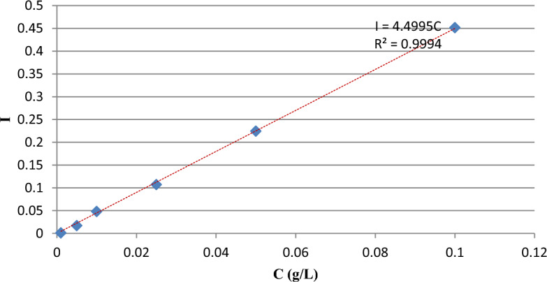
The calibration curve of drug in DM water.

For solubility calculations, the following equations were employed:

$$y_2=\frac{n_{\mathit{drug}}}{n_{\mathit{drug}}+n_{C{O}_2}}$$ 1

where $n_{\text{drug}}$ and $n_{{\text{CO}}_2}$ represent the moles of codeine phosphate and CO₂, respectively.

Moreover, these quantities are defined as follows:

$$n_{\text{drug}}=\frac{C_s·V_s}{M_s}$$ 2

$$n_{{\text{CO}}_2}=\frac{V_1·\rho }{M_{{\text{CO}}_2}}$$ 3

In the above relations, $C_{\text{s}}$ is defined as the drug concentration in saturated sample vial in g/L. Also, the volume of the sampling loop and vial collection are expressed as V₁(L) = 600 $\times$ 10^–6 m³ and V_s(L) = 5 $\times$ 10^–3 m³, respectively. The $M_s$ and $M_{C{O}_2}$ are the molecular weights of the codeine phosphate drug (component 2) and CO₂, respectively.

Solubility can be also expressed as:

$$S=\frac{C_S{V}_s}{V_1}$$ 4

where, one can find the relation between S and $y_2$ as follows:

$$S=\frac{\rho M_s}{M_{C{O}_2}}\frac{y_2}{1-y_2}$$ 5

Codeine phosphate’s solubility was determined using a UV–visible spectrophotometer (Model UNICO-4802, double beam, with multipurpose software, USA), with DM water as the solvent.

Modeling

The solubility data obtained in this study were correlated with one equation of state (EoS), five density-based models, and three ELM models. we considered the Peng-Robinson (PR) EoS. In the case of density-based modeling, several well-known models, namely Chrastil, Mendez-Santiago, Teja (MT), Bartle et al., Sodeifian et al., and Reddy-Garlapati were employed. Three forms of ELMs with different parameters were used for data fitting. Detailed information about all the models considered in this work is discussed in the following sections.

EoS modeling

This model is an extension to the model framework suggested by Schmitt⁵³ and Reid and Estévez et al.⁵⁴. PR EoS was used for the modeling. Solubility of codeine phosphate (solute, component 2) in SC-CO₂ (solvent, component 1) is expressed as⁵⁵

$${\text{y}}_2=\frac{P_2^S{\widehat{\varphi }}_2^S}{P{\widehat{\varphi }}_2^{SC-C{O}_2}}exp\left[\frac{\left(P-P_{2i}^S\right)v_S}{\mathit{RT}}\right]$$ 6

where $P_2^s$, ${\widehat{\varphi }}_2^{SC-C{O}_2}$, ${\widehat{\varphi }}_2^S$ $P$, $v_2$, $T$ and R, are sublimation pressure, solid solute fugacity coefficient, saturation fugacity coefficient, system pressure, drug molar volume, system temperature and universal gas constant, respectively. The required equation for the solid solute fugacity coefficient in the SC-CO₂ (${\widehat{\varphi }}_2^{SC-C{O}_2}$) is calculated using PR EoS. It is obtained from the following thermodynamic equation.

$$ln\left({\widehat{\phi }}_2^{SC-C{O}_2}\right)=\frac{1}{\mathit{RT}}\underset{v}{\overset{\infty }{\int }}\left[{\left(\frac{\partial P}{\partial N_i}\right)}_{T,V,N_1}-\frac{\mathit{RT}}{v}\right]dv-lnZ$$ 7

Equation (8) represents the fugacity coefficients expression for PR EoS.

$$ln\left({\widehat{\phi }}_2^{SC-C{O}_2}\right)=b_2/b\left(Z-1\right)-ln\left(P\left(V-b\right)/RT\right)-a/(2\sqrt{2}RTb)\left\{[2(a_{12}{y}_1+a_2{y}_2)/a]-b_2/b\right\}ln\left[\frac{V+2.414b}{V-0.414b}\right]$$ 8

For modeling tasks, critical temperature, critical pressure, centric factor, molar volume, and sublimation pressures of the codeine phosphate are required. Unfortunately, they are unavailable for this typical drug. Therefore, to overcome this drawback, the following assumptions are applied.

Assumption 1

Solute in the solvent is very dilute. Thus, the required ${\widehat{\varphi }}_2^{SC-C{O}_2}$ is obtained by applying William J. Schmitt and Robert C. Reid assumptions to Eq. (8) (i.e., for dilute system $z\to z_1$, $a\to a_1$ and $b\to b_1$). Thus, ${\widehat{\varphi }}_2^{SC-C{O}_2}$ PR EoS (Eq. 8) is reduced to Eq. (9). In which solute parameters are adjustable (i.e., $a_2$ and $b_2$)⁵³.

$$ln\left({\widehat{\phi }}_2^{SC-C{O}_2}\right)\approx {b_2/b}_1\left(Z_1-1\right)-ln\left(P\left(V_1-b_1\right)/RT\right)-a_1/(2\sqrt{2}RT{b}_1)\left\{[2(a_2)/a_1]-b_2/b_1\right\}ln\left[\frac{V_1+2.414b_1}{V_1-0.414b_1}\right]$$ 9

Assumption 2

The molar volume of solute ($v_2$) is a function of SC-CO₂ (solvent) density (${\rho }_1$)⁵⁶ and in this work the following expression is used

$$v_2=K_1+K_2{\rho }_1+K_3{\rho }_1^2$$ 10

where $K_1,$$K_2,$$K_3$ have units are m³/mol, m⁶/mol kg, m⁹/mol kg², respectively.

Assumption 3

The sublimation pressure of the solute is expressed as a function of temperature, and it is expressed as Eq. (11)⁵⁵

$$Rln\left(P_A^{\mathit{sub}}\right)=\beta +\frac{\gamma }{T}+{\mathrm{\Delta }}_{\mathit{sub}}\delta ln\left(\frac{T}{298.15}\right)$$ 11

where $\beta$, $\gamma$ and ${\mathrm{\Delta }}_{\mathit{sub}}\delta$ are sublimation pressure expression coefficients. They are substituting Eqs. (9)–(11), in Eq. (6), results in the solubility model based on PR EoS in terms of pressure, temperature, density, and some adjustable parameters. The adjustable parameters are $a_2$, $b_2$, $\beta$, $\gamma$,${\mathrm{\Delta }}_{\mathit{sub}}\delta$,$K_1$,$K_2$ and $K_3$. These parameters are treated as temperature-independent in the temperature range considered in the present work. The adjustable parameters are obtained by regression with experimental data.

For the data regression, the objective function, Eq. (12), is used⁵⁷

$$OF=\sum _{i=1}^N\frac{\left|y_{2i}^{exp}-y_{2i}^{\mathit{calc}}\right|}{y_{2i}^{exp}}$$ 12

where $y_{2i}^{exp}$ is the experimental mole fraction of solute, and $y_{2i}^{\mathit{calc}}$ is the model predicted mole fraction of solute.

Density-based modeling

Chrastil model^58–60

Solute concentration and solvent density are related as follows:

$$c_m={\left({\rho }_{m1}\right)}^{\kappa }exp\left(A_1+B_1/T/K\right)$$ 13

where $c_m$ is the mass concentration of solute,${\rho }_{m1}$ is the mass concentration of solvent, and $\kappa$,$A_1$ and $B_1$ are model constants.

Equation (1) can be rearranged to mole fraction as follows:

$$\frac{c_m}{{\rho }_{m1}}\frac{M_{\mathit{ScF}}}{M{}_{\mathit{Solute}}}=\frac{M_{\mathit{ScF}}}{M{}_{\mathit{Solute}}}{\left({\rho }_1\right)}^{\kappa -1}exp\left(A_1+B_1\left./\phantom{B_{1}T/K}\right)T/K\right)$$ 14

where $M_{\mathit{ScF}}$, $M{}_{\mathit{Solute}}$ and $c_m/M_{\mathit{solute}}$ are molar mass of SCF, molar mass of solute, and molar concentration of solute ($c$), respectively. Also,${\rho }_{m1}/M_{\mathit{ScF}}$ and $\kappa$ are molar concentration of solvent(${\rho }_1$), and association number, respectively. Furthermore, $A_1$ and $B_1$ are model constants.

$$moleratio=\frac{c}{{\rho }_1}=\frac{M_{\mathit{ScF}}}{M{}_{\mathit{Solute}}}{\left({\rho }_1\right)}^{\kappa -1}exp\left(A_1+B_1/T/K\right)$$ 15

Mole fraction ($y_2$) and mole ratios are related as follows:

$$\frac{c}{{\rho }_1}=\frac{y_2}{1-y_2}$$ 16

$$y_2=moleratio/\left[1+moleratio\right]$$ 17

$$y_2=\frac{M_{\mathit{ScF}}}{M{}_{\mathit{Solute}}}{\left({\rho }_1\right)}^{\kappa -1}exp\left(A_1+B_1/T/K\right)\left./\phantom{\frac{M_{\mathit{ScF}}}{M{}_{\mathit{Solute}}}{\left({\rho }_1\right)}^{\kappa -1}exp\left(A_1+B_1\left./\phantom{B_{1}T/K}\right)T/K\right)\left[1+\frac{M_{\mathit{ScF}}}{M{}_{\mathit{Solute}}}{\left({\rho }_1\right)}^{\kappa -1}exp\left(A_1+B_1/T/K\right)\right]}\right)\left[1+\frac{M_{\mathit{ScF}}}{M{}_{\mathit{Solute}}}{\left({\rho }_1\right)}^{\kappa -1}exp\left(A_1+B_1/T/K\right)\right]$$ 18

where $\kappa$,$A_1$ and $B_1$ are the model constants and their units are dimensionless, dimensionless and K, respectively.

Méndez-Santiago and Teja (MT) model⁶¹

This model can generally be used for checking thermodynamic consistency. It is stated as Eq. (19) and when $Tln\left(y_{2}P\right)-C_{2}T$ vs. ${\rho }_1$ is established, all data points fall around a single straight line

$$Tln\left(y_{2}P\right)=A_2+B_2·{\rho }_1+C_{2}T$$ 19

where $A_2$, $B_2$ and $C_2$ are the model constants and their units are K, K m³/kg and dimensionless, respectively

Bartle et al. model⁶²

According to the model, the solubility is expressed as Eq. (20)

$$ln\left(\frac{y_2·P}{P_{\mathit{ref}}}\right)=A_3+\frac{B_3}{T}+C_3\left({\rho }_1-{\rho }_{\mathit{ref}}\right)$$ 20

where the pressure ($P_{\mathit{ref}}$) and density for reference states (${\rho }_{\mathit{ref}}$) are considered 0.1 MPa, and 700 kg m⁻³. Also, $A_3$, $B_3$ and $C_3$ are the model constants and their units are dimensionless, K and m³/kg, respectively. From the constant $B_3$, sublimation enthalpy can be obtained (i.e.,${\mathrm{\Delta }}_{\mathit{sub}}H=-B_{3}R$ J/mol).

Sodeifian et al. model⁶³

According to this model, the solubility is represented by Eq. (21)

$$y_2=A_4+B_4\frac{P^2}{T}+C_{4}ln\left({\rho }_{1}T\right)+D_4{\rho }_{1}ln\left({\rho }_1\right)+E_{4}Pln\left(T\right)+F_4\frac{ln\left({\rho }_1\right)}{T}$$ 21

where $A_4$, $B_4$, $C_4$, $D_4$, $E_4$ and $F_4$ are the model constants and their units are dimensionless, K/MPa², dimensionless, m³/Kg, 1/MPa and K, respectively.

Reddy-Garlapati model⁶⁴

According to the model, the solubility is expressed as Eq. (22)

$$y_2=\left(A_5+B_5{P}_r+C_5{P}_r^2\right)T_r+(D_5+E_5{P}_r+F_5{P}_r^2)$$ 22

where $A_5$ $B_5$, $C_5$, $D_5$, $E_5$ and $F_5$ are the model constants and all are dimensionless quantities;$P_r$ is reduced pressure and $T_r$ is reduced temperature.

Expanded Liquid Models (ELMs)

This section deals with models under the solid–liquid equilibrium model (also known as ELMs). It relies on the solution theory, where SC-CO₂ was considered an expanded liquid with infinite dissolved codeine phosphate. The essential solubility expression is given by^65–68

$$y_2=\frac{1}{{\gamma }_2^{\infty }}\frac{f_2^S}{f_2^L}$$ 23

where ${\gamma }_2^{\infty }$ is the activity coefficient of solute at infinite dilution,$f_2^S$, $f_2^L$ are fugacity of codeine phosphate compound in the solid phase and expanded liquid phase, respectively. The basic equation for the fugacity ratio is represented by

$$ln\left(\frac{f_2^S}{f_L^L}\right)=\frac{\mathrm{\Delta }{H}_2^m}{\mathit{RT}}\left(\frac{T}{T_m}-1\right)-\underset{T_m}{\overset{T}{\int }}\frac{1}{R{T}^2}\left[\underset{T_m}{\overset{T}{\int }}\left[\mathrm{\Delta }{C}_p\right]dT\right]dT$$ 24

where $\mathrm{\Delta }{C}_p$ implies the difference between the heat capacity of solid and expanded liquid states. When Eqs. (23 and 24) are combined, the solubility expression for ELM is obtained as Eq. (25)

$$y_2=\frac{1}{{\gamma }_2^{\infty }}exp\left[\frac{\mathrm{\Delta }{H}_2^m}{\mathit{RT}}\left(\frac{T}{T_m}-1\right)-\underset{T_m}{\overset{T}{\int }}\frac{1}{R{T}^2}\left[\underset{T_m}{\overset{T}{\int }}\left[\mathrm{\Delta }{C}_p\right]dT\right]dT\right]$$ 25

The solubility expression may be estimated with and without $\mathrm{\Delta }{C}_p$ term. In the following section, three cases are presented. For all three cases, a unique expression for ${\gamma }_2^{\infty }$ used^23,69 was $exp\left(l_1+l_2(p/(RT)\right)+l_3{(p/(RT))}^2)$.

Case 1. $\mathrm{\Delta }{C}_p=0$.

The solubility expression for this case is written as

$$y_2=exp\left[\frac{\mathrm{\Delta }{H}_2^m}{\mathit{RT}}\left(\frac{T}{T_m}-1\right)\right]/exp\left(l_1+l_2\left(\frac{p}{\mathit{RT}}\right)+l_3{\left(\frac{p}{\mathit{RT}}\right)}^2\right)$$ 26

Thus Eq. (26) has three maximum parameters (l₁, l₂ and l₃).

Case 2. $\mathrm{\Delta }{C}_p=\text{contant}$. Consider the constant $\mathrm{\Delta }{C}_p$ is D²³.

The solubility expression for this case iswritten as

$$y_2=exp[\frac{\mathrm{\Delta }{H}_2^m}{\mathit{RT}}\left(\frac{T}{T_m}-1\right)-\raisebox{1ex}{$D$}\!\left/ \!\raisebox{-1ex}{$R$}\right.\left[ln\left(\frac{T}{T_m}\right)-T_m\left(\frac{1}{T_m}-\frac{1}{T}\right)\right]/exp\left(l_1+l_2\left(\frac{p}{\mathit{RT}}\right)+l_3{\left(\frac{p}{\mathit{RT}}\right)}^2\right)$$ 27

Thus Eq. (27) has four maximum of parameters ($D$, l₁, l₂ and l₃) and respective units are J/mole K, dimensionless, J/mole MPa and J²/mole² MPa², respectively.

Case 3. $\mathrm{\Delta }{C}_p=f(T)$.

Generally,$C_p$ it is a third-order polynomial equation in temperature equation; however, a recent study on solubility modeling shows that a good fit is achieved with the second-order polynomial. Thus, it is assumed that the $\mathrm{\Delta }{C}_p$ quadratic function in temperature as Eq. (28)⁷⁰

$$\mathrm{\Delta }{C}_p={\beta }_1+{\beta }_{2}T+{\beta }_3{T}^2$$ 28

Integral evaluation of Eq. (25) by substituting Eq. (28) results in Eq. (29)

$$\begin{array}{cc}\hfill ln\left(\frac{f_2^S}{f_L^L}\right)& =\frac{\mathrm{\Delta }{H}_2^m}{\mathit{RT}}\left(\frac{T}{T_m}-1\right)-\frac{{\beta }_1}{R}\left[ln\left(\frac{T}{T_m}\right)-T_m\left(\frac{1}{T_m}-\frac{1}{T}\right)\right]-\frac{{\beta }_2}{2R}\left[\left(T-T_m\right)-T_m^2\left(\frac{1}{T_m}-\frac{1}{T}\right)\right]\hfill \\ \hfill & -\frac{{\beta }_3}{3R}\left[\left(\frac{T^2}{2}-\frac{T_m^2}{2}\right)-T_m^3\left(\frac{1}{T_m}-\frac{1}{T}\right)\right]\hfill \\ \hfill \end{array}$$ 29

Thus, the solubility expression for this case is written as

$$\begin{array}{c}{y}_2=exp[\frac{\mathrm{\Delta }{H}_2^m}{\mathit{RT}}\left(\frac{T}{T_m}-1\right)-\frac{{\beta }_1}{R}\left[ln\left(\frac{T}{T_m}\right)-T_m\left(\frac{1}{T_m}-\frac{1}{T}\right)\right]-\frac{{\beta }_2}{2R}\left[\left(T-T_m\right)-T_m^2\left(\frac{1}{T_m}-\frac{1}{T}\right)\right]\\ -\frac{{\beta }_3}{3R}\left[\left(\frac{T^2}{2}-\frac{T_m^2}{2}\right)-T_m^3\left(\frac{1}{T_m}-\frac{1}{T}\right)\right]]/exp\left(l_1+l_2\left(\frac{p}{\mathit{RT}}\right)+l_3{\left(\frac{p}{\mathit{RT}}\right)}^2\right)]\\ \end{array}$$ 30

In Eq. (30), six parameters are there and they are ${\beta }_1$,${\beta }_2$,${\beta }_3$, l₁, l₂ and l₃ and their units are J/K kg, J/K²kg, J/K³kg, dimensionless, J/mole MPa and J²/mole² MPa², respectively. These parameters are optimally fitted to experimental solubility data by minimizing the error with the help of the objective function defined in Eq. (12). It is also important to note that all three expressions for solubility are explicit functions of composition.

Results and discussion

The present study reports the measured solubilities of codeine phosphate (C₁₈H₂₁NO₃) in supercritical carbon dioxide (SC-CO₂) at temperatures of 308, 318, 328, and 338 K, spanning a pressure range of 12–27 MPa. Three types of models mentioned in the previous section were used in data correlation. The correlation task was carried out in MATLAB 2019® using the inbuilt fminsearch algorithm. The optimization algorithm minimized the error and was used for parameter estimation for all the models mentioned in the previous section. The measured data are shown in Table 2. The solvent density was obtained from the NIST database⁷¹. Considering the order of magnitude of codeine phosphate solubility in SC-CO₂, supercritical anti-solvent methods can be regarded an appropriate choice for producing fine particles of this drug.

Table 2.

Solubility of crystalline codeine phosphatein SC-CO₂ at various temperatures and pressures.

Temperature (K)a	Pressure (MPa)a	Density of SC-CO2 (kg/m3)1	y2 × 105 (Mole fraction)	Experimental standard deviation, S(ȳ) × (105)	S (Equilibrium solubility) (g/L)	Expanded uncertainty of Mole fraction (105 U)
308	12	769	1.297	0.021	0.090	0.072
	15	817	1.615	0.014	0.119	0.078
	18	849	1.702	0.022	0.131	0.086
	21	875	1.754	0.083	0.138	0.113
	24	896	1.897	0.031	0.153	0.104
	27	914	1.991	0.055	0.164	0.103
318	12	661	1.387	0.038	0.083	0.099
	15	744	2.614	0.091	0.176	0.041
	18	791	2.742	0.021	0.196	0.130
	21	824	3.158	0.077	0.235	0.108
	24	851	3.422	0.093	0.263	0.109
	27	872	3.817	0.040	0.300	0.106
328	12	509	1.891	0.082	0.087	0.115
	15	656	3.594	0.011	0.213	0.124
	18	725	3.949	0.088	0.259	0.150
	21	769	4.284	0.062	0.298	0.127
	24	802	4.521	0.095	0.327	0.176
	27	829	5.441	0.063	0.407	0.171
338	12	388	2.294	0.071	0.080	0.178
	15	557	3.959	0.081	0.199	0.142
	18	652	4.395	0.033	0.259	0.108
	21	710	4.927	0.128	0.316	0.137
	24	751	5.521	0.141	0.375	0.173
	27	783	6.502	0.065	0.459	0.115

The experimental standard deviation was obtained by $S\left(y_k\right)=\sqrt{\frac{{\sum }_{j=1}^n{\left(y_j,-,\overline{y}\right)}^2}{n-1}}$. Expanded uncertainty (U) and the relative combined standard uncertainty (u_combined/y) are defined, respectively, as follows: (U) = k*u_combined (k = 2) and $\raisebox{1ex}{$u_{\mathit{combined}}$}\!\left/ \!\raisebox{-1ex}{$y$}\right.=\sqrt{\sum _{i=1}^N{\left(P_{i}u\left(x_i\right)/x_i\right)}^2}$. In this research, u(x_i) was considered as standard uncertainties of temperature, pressure, mole fraction, volumes and absorption. P_i, sensitivity coefficients, are equal to the partial derivatives of y equation (Eq. 1) with respect to the x_i.

^aStandard uncertainty u are u(T) =  ± 0.1 K; u(p) =  ± 1 bar.

The value of the coverage factor k = 2 was chosen on the basis of the level of confidence of approximately 95 percent for calculating the expanded uncertainty.

The solubility of codeine phosphate in SC-CO₂ vs. pressure is depicted in Fig. 3. From the solubility plot, it is evident that a cross-over pressure is not observed for codeine phosphate. Since conducting experimental investigations at each required condition (pressure and temperature) is tedious, modeling becomes necessary. Therefore, modeling was performed in all three modes. Numerous equations of state (EoS) are available in the literature for modeling solubility data. However, the PR EoS was selected in this work due to its success in modeling the solubilities of solid substances in supercritical fluids (SCFs)^53–55,70. When correlating the data, the PR EoS model parameters were treated as temperature-independent over 308–338 K. The objective function indicated in Eq. (12) was utilized for data correlation, and all the adjustable parameters were obtained through regression with experimental data. Table 3 presents the correlation constants of the PR EoS model. Sublimation enthalpies at 308, 318, 328, and 338 K were calculated from the vapor pressure expression constants using the following relation:

$${\mathrm{\Delta }}_{\mathit{sub}}H=\left(-\gamma +{\mathrm{\Delta }}_{\mathit{sub}}\delta T\right)R\text{J}/\text{mol}$$ 31

Figure 3.

Codeine phosphate solubility in SC-CO₂, $y_2$ versus P (MPa).

Table 3.

Correlation constant of EoS model.

Name of the model	Parameters	AARD%	$R^2$	$R_{\mathit{adj}}^2$
PREoS	$a_1$ = 2.3463 × 10–4	8.61	0.918	0.899
	$b_1$ = 4.2013 × 10–4
	$\beta$ = 23.310
	$\gamma$ = − 9127.5
	${\mathrm{\Delta }}_{\mathit{sub}}\delta$ = − 5.9988
	$K_1$ = 7.516 × 10–4
	$K_2$ = − 7.3793 × 10–8
	$K_3$ = − 7.8339 × 10–11
Estimated Sublimation Enthalpies at T (K)	Sublimation Enthalpy (kJ/mol) Estimated using ${\mathrm{\Delta }}_{\mathit{sub}}H=(-\gamma +{\mathrm{\Delta }}_{\mathit{sub}}\delta T)R$	Average Sublimation Enthalpy in kJ/mol
308	60.524	59.776
318	60.026
328	59.527
338	59.028

The estimated sublimation enthalpies are presented in Table 3. The correlating ability of the equation of state (EoS) method is depicted in Fig. 3.

When considering density-based models for data correlation, the Chrastil model (Eq. 18), treated constants as independent variables, and their values were determined through regression with experimental data. The obtained constants are reported in Table 4. The correlating ability of the Chrastil model is illustrated in Fig. 4. Reasonable fit is observed when the data is represented as y₂ versus ${\rho }_1$, this confirms the applicability of the Chrastil model to the solubility data^72,73. From the parameters of the Chrastil model, the total enthalpy for codeine phosphate was derived, and its value is reported in Table 5.

Table 4.

Correlation constant of density-based models.

Name of the model	Parameters	AARD%	$R^2$	$R_{\mathit{adj}}^2$
Chrastil	$\kappa$ = 2.8403	9.48	0.902	0.897
	$A_1$ = − 4.0221
	$B_1$ = − 5284.7
MT model	$A_2$ = − 8817.9	11.8	0.891	0.886
	$B_2$ = 17.341
	$C_2$ = 15.802
Bartle et al.	$A_3$ = 17.257	12.3	0.894	0.889
	$B_3$ = − 7326
	$C_3$ = 5.2862 × 10–3
Sodeifian et al.	$A_4$ = − 0.015589	8.52	0.936	0.933
	$B_4$ = − 3.2068 × 10–5
	$C_4$ = 0.40046
	$D_4$ = 1.1612 × 10–3
	$E_4$ = − 4.7474 × 10–3
	$F_4$ = − 1005.1
Reddy and Garlapati	$A_5$ = 1.68 × 10–4	9.48	0.954	0.952
	$B_5$ = − 1.2939 × 10–6
	$C_5$ = 2.2027 × 10–5
	$D_5$ = − 2.0904 × 10–4
	$E_5$ = 3.8763 × 10–5
	$F_5$ = − 2.8153 × 10–5

Figure 4.

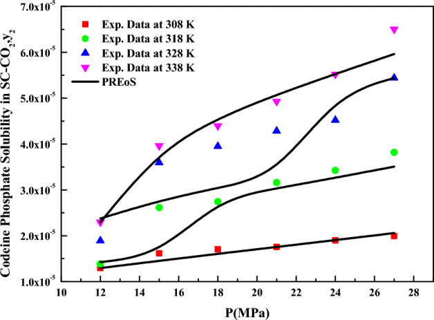
Codeine phosphate solubility in SC-CO₂, $y_2$ versus P (MPa). Symbols are experimental points; lines are PREoS model fit.

Table 5.

Thermodynamic parameters of codeine phosphate-SC-CO₂ system.

Model	Name of property
	Total enthalpy ΔHtotal (kJ/mol)	Enthalpy of sublimation ΔHsub (kJ/mol)	Enthalpy of solvation ΔHsol (kJ/mol)
Chrastil model	43.94a		− 16.97d
Bartle et al. model		60.91b (average value)	− 15.84e
PREoS		59.78c (average value)

^dObtained as a result of difference between ΔH_sub^b and ΔH_total^a.

^eObtained as a result of difference between ΔH_sub^c and ΔH_total^a.

The results for data fitting of the MT model (Eq. 19) are presented in Fig. 6, and the corresponding parameters are reported in Table 4. The correlating ability of the MT model is evident in Fig. 5, where linear plots are observed when the data is plotted as $T/Kln\left(y_2·P\right)-C_{2}T$ versus ${\rho }_1$ (Fig. 6), this further confirms the suitability of the MT model for the solubility data^72,73. Similarly, the model proposed by Bartle et al. (Eq. 20) was correlated with solubility data, and the obtained results are reported in Table 4. Linear plots are also observed when the data is represented as $ln\left(y_{2}P/P_{\mathit{ref}}\right)$ versus $\left({\rho }_1-{\rho }_{\mathit{ref}}\right)$ (Fig. 7),confirming the applicability of the Bartle et al. model to the solubility data^72,73.From the parameters of the Bartle et al. model, the vaporization enthalpy was determined, and its value is reported in Table 5.

Figure 6.

$Tln(y_{2}P)-C_{2}T$ vs. ${\rho }_1$(kg m⁻³). Symbols are experimental points, and lines are MT model fit.

Figure 5.

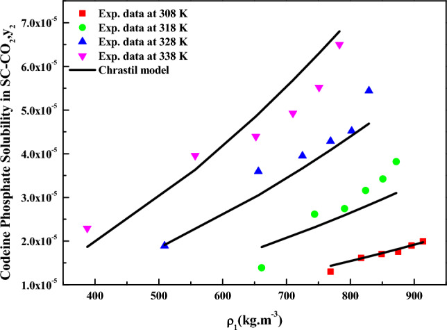
Codeine Phosphate Solubility, y₂ versus ${\rho }_1$. Symbols are experimental points, and lines are Chrastil model fit.

Figure 7.

$ln(y_{2}P/P_{\mathit{ref}})$ versus $({\rho }_1-{\rho }_{\mathit{ref}})$ kg m⁻³. Symbols are experimental points, and lines are Bartle et al., model fit.

The solvation enthalpy was computed using the values of total and vaporization enthalpies, and the computed solvation enthalpy values are reported in Table 5. Notably, there is good agreement between the calculated average sublimation enthalpies from the PR EoS model (59.78 kJ/mol, as derived from Tables 3 and 5) and the calculated sublimation enthalpies from the Bartle et al. model (60.91 kJ/mol, as derived from Table 5). This suggests that using the PR EoS method in this study can yield meaningful correlation constants. However, the PR EoS accuracy decreases as the temperature increases from 308 to 338 K, possibly due to the temperature dependency of adjustable parameters. Figure 8 depicts the data fitting achieved using the Sodeifian and Reddy–Garlapati models.

Figure 8.

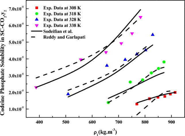
Codeine phosphate solubility in SC-CO₂, $y_2$ versus ${\rho }_1$(kg m⁻³). Symbols are experimental points, lines are Sodeifian and Reddy-Garlapati model’s fit.

Three forms of expanded liquid models, precisely Eqs. (26), and (30), underwent evaluation with experimental data using the objective function mentioned in Eq. (12). Among these models, Eq. (30), which possesses the highest number of parameters, strongly agrees with the experimental data. Table 6 presents all the parameters associated with the expanded liquid models, and Fig. 9 shows the data correlation capabilities of these models.

Table 6.

Correlation constant of ELM models.

Name of the model	Parameters	AARD%	$R^2$	$R_{\mathit{adj}}^2$
ELM1	$l_1$ = 10.134	11.1	0.919	0.890
	$l_2$ = − 598.37
	$l_3$ = 31,626
ELM2	$l_1$ = 10.196	11.0	0.919	0.891
	$l_2$ = − 600.81
	$l_3$ = 31,962
	$D$ = − 11.85
ELM3	$l_1$ = 7.4325	8.89	0.952	0.935
	$l_2$ = − 609.58
	$l_3$ = 32,270
	${\beta }_1$ = 224,920
	${\beta }_2$ = − 1269.3
	${\beta }_3$ = 13.166

Figure 9.

Codeine phosphate solubilities in SC-CO₂, $y_2$ versus ${\rho }_1$(kg m⁻³). Symbols are experimental points; lines are ELMs model’s fit.

The quality of data fit is contingent upon the number of parameters employed in the model. The Akaike Information Criterion (AIC) and the corrected AIC (AICc) are utilized to discern the optimal model. AIC_cis computed based on AIC^74–77, mathematical criteria commonly employed for assessing the compatibility of a solubility model with the corresponding solubility data. In statistics, these criteria compare solubility models and determine whichbest fits the data. AIC is appropriate when the data set comprises more than 40 data points, whereas AIC_c is preferred when the data set contains fewer than 40 data points^75,76. The following is relation between AIC and AIC_c. Additionally, the adjustable or mode parameters may be determined by different algorithms or methods such as nonlinear regression models^78,79.

$$AI{C}_c=AIC+\frac{2Q\left(Q+1\right)}{N-Q-1}$$ 32

In Eq. (32), N represents the number of experimental data points, Q denotes the adjustable constants of the model, and AIC is defined as the sum of $Nln\left(\mathit{SSE}/N\right)$&$2Q$, where SSE stands for the sum of squared error. Table 7 displays all the computed values, revealing that Eq. (30) exhibits the lowest AIC_c value, establishing it as the most suitable model for the given data.

Table 7.

Statistical values (AIC and AIC_c) of all models.

Name of the model	RMSE	SSE	AIC	AICc
EoS model	3.945 × 10–6	4.359 × 10–10	− 578	− 567.97
Chrastil	4.0383 × 10–3	3.5878 × 10–4	− 261	− 259.46
MT model	5.6176 × 10–6	6.9426 × 10–10	− 576	− 575.19
Bartle et al.	5.4034 × 10–6	6.4233 × 10–10	− 578	− 577.06
Sodeifian et al.	4.0748 × 10–6	3.6529 × 10–10	− 586	− 580.86
Reddy-Garlapati	3.3912 × 10–6	2.5301 × 10–10	− 595	− 587.67
ELM1	4.2894 × 10–6	4.4157 × 10–10	− 587	− 586.05
ELM2	4.2145 × 10–6	4.263 × 10–10	− 586	− 583.99
ELM3	3.2394 × 10–6	2.5185 × 10–10	− 595	− 589.79

The best model has the lowest AIC_c value. The six-parameter ELM model is identified as the optimal choice, while based on AIC_c, the Chrastil model exhibits a weaker correlation than the other models considered in this study.

Conclusion

This research presents, for the first time, solubility data of codeine phosphate in SC-CO₂ measured at various conditions ranging between 308 and 338 K and 12–27 MPa. The measured data was found to vary within the range of (1.297–6.502) × 10^–5 in mole fraction. The obtained solubility data were modeled using the PREoS model, with solute properties as one of the adjustable constants. Among the density models, the Chrastil, MT, and Bartle et al. models effectively captured the data. From the model constants, the enthalpies of the SC-CO₂-codeine phosphate mixture were determined. Three expanded liquid models (ELMs) were applied to the solubility data. The model results indicate that all the expanded liquid models (ELMs) reasonably fit the data compared to the PR EOS and density models. Finally, AICc analysis indicates that the six-parameter ELM model is the most suitable model for data correlation. Considering the order of magnitude of solubility of codeine phosphate in SC-CO₂, supercritical anti-solvent methods can be considered an appropriate choice for producing fine particles of this drug.

List of symbols

$A_1,B_1$

Chrastil’s model parameters (dimensionless, K)

$A_2,B_2,C_2$

MT model parameters (K, K m³/kg, dimensionless)

$A_3,B_3,C_3$

Bartle’s model parameters (dimensionless, K m³/kg)

$A_4,B_4,C_4,D_4,E_4,F_5$

Sodeifian’s model parameters (dimensionless, K/MPa², m³/kg K, m⁶/kg², 1/K MPa, K m³/kg)

$A_5,B_5,C_5,D_5,E_5,F_5$

Reddy-Garlapati’s model parameters (all are dimensionless)

AARD%

Average absolute relative deviation percentage

AIC

Akaike information criterion

AIC_c

Corrected AIC

C_s

The drug in the sample in vial (g/L)

D

Equation (27) parameter (J/molK)

E1 to E14

Symbols used in the experimental setup

${\text{H}}_{\text{sol}},{\text{H}}_{\text{sub}},{\text{H}}_{\text{total}}$

Enthalpy (J/mol or kJ/mol)

$K_1,K_2,K_3$

Equation (10) parameters (m³/mol, m⁶/mol kg, m⁹/mol kg²)

$l_1,l_2,l_3$

Activity coefficient parameters (dimensionless, J/mole MPa, J²/mole² MPa²)

${\text{M}}_{{\text{CO}}_2},{\text{M}}_{\text{Solute}}$

The molar mass of CO₂ and drug solute (g/mol)

$n_{{\text{CO}}_2}$

CO₂ moles

$n_{d\mathrm{rug}}$

Drug moles

N

Data points

NIST

National Institute of Standards and Technology

OF

Objective function

Q

Equation (32) parameter

P

Pressure (MPa)

${\text{P}}_{\text{c}},{\text{P}}_{\text{r}}$

Critical (Pa or MPa) and reduced pressures

Ps

Sublimation pressure (Pa or MPa)

R

Universal gas constant, 8.314 J/(mol K)

RMSD

Root mean square deviation

S

Solubility (kg/m₃; kg mol/m₃)

SSE

The sum of squares error

SC-CO₂

Supercritical carbon dioxide

$\text{T},{\text{T}}_{\text{c}}$

System temperature and critical temperature (K)

$v_1{,v}_2,v_s$

Molar volume (m³/mol)

$V_1,V_{\text{s}}$

Sampling loop and collection vial volumes, in (μL)

$y_2$

Drug solute solubility in mole fraction

Greek symbols

$\beta$

Equation (11) parameters (dimensionless)

${\beta }_1,{\beta }_2\text{and}{\beta }_3$

Equation (30) parameters (J/K kg, J/K²kg and J/K³kg)

$\gamma$

Equation (11) parameters (K)

$\rho ,{\rho }_r$

Density (kg/m³, kgmol/m³), reduced density

$\kappa$

Association numbers

${\mathrm{\Delta }}_{\mathit{sub}}\delta$

Equation (11) parameters (dimensionless)

Subscript

C

Critical

r

Reduced

Sol

Solvation

Sub

Sublimation

Total

Total

Superscript

S

Saturation

Author contributions

G.S. Conceptualization, Methodology, Validation, Investigation, Supervision, Project administration, Writing-review & editing; C.G. Methodology, Investigation, Software, Writing-original draft; M.A.N Validation, Measurement, Resources; F.R. Investigation, Software, Validation; A.R. Resources.

Data availability

Upon request, the data can be obtained from the corresponding author.

Competing interests

The authors declare no competing interests.

References

- 1.Tabernero A, del Valle EMM, Galán MA. Supercritical fluids for pharmaceutical particle engineering: Methods, basic fundamentals and modelling. Chem. Eng. Process Intensif. 2012;60:9–25. doi: 10.1016/j.cep.2012.06.004. [DOI] [Google Scholar]
- 2.Subramaniam B, Rajewski RA, Snavely K. Pharmaceutical processing with supercritical carbon dioxide. J. Pharm. Sci. 1997;86(8):885–890. doi: 10.1021/js9700661. [DOI] [PubMed] [Google Scholar]
- 3.Mukhopadhyay M. Partial molar volume reduction of solvent for solute crystallization using carbon dioxide as antisolvent. J. Supercrit. Fluids. 2003;25(3):213–223. doi: 10.1016/S0896-8446(02)00147-X. [DOI] [Google Scholar]
- 4.Elvassore NK. Pharmaceutical processing with supercritical fluids. In: Bertucco A, editor. High Pressure Process Technology: Fundamentals and Applications. Elsevier Science; 2001. pp. 612–625. [Google Scholar]
- 5.Gupta, R. B & Chattopadhyay, P. Method of forming nanoparticles and microparticles of controllable size using supercritical fluids and ultrasound. US patent No. 20020000681 (2002).
- 6.Reverchon E, Adami R, Caputo G, De Marco I. Spherical microparticles production by supercritical antisolvent precipitation: interpretation of results. J. Supercrit. Fluids. 2008;47(1):70–84. doi: 10.1016/j.supflu.2008.06.002. [DOI] [Google Scholar]
- 7.Sodeifian G, Ardestani NS, Sajadian SA, Panah HS. Experimental measurements and thermodynamic modeling of Coumarin-7 solid solubility in supercritical carbon dioxide: Production of nanoparticles via RESS method. Fluid Phase Equilib. 2019;483:122–143. doi: 10.1016/j.fluid.2018.11.006. [DOI] [Google Scholar]
- 8.Sodeifian G, Sajadian SA, Ardestani NS, Razmimanesh F. Production of loratadine drug nanoparticles using ultrasonic-assisted rapid expansion of supercritical solution into aqueous solution (US-RESSAS) J. Supercrit. Fluids. 2019;147:241–253. doi: 10.1016/j.fluid.2018.05.018. [DOI] [Google Scholar]
- 9.Sodeifian G, Sajadian SA, Ardestani NS. Determination of solubility of Aprepitant (an antiemetic drug for chemotherapy) in supercritical carbon dioxide: Empirical and thermodynamic models. J. Supercrit. Fluids. 2017;128:102–111. doi: 10.1016/j.supflu.2017.05.019. [DOI] [Google Scholar]
- 10.Sodeifian G, Razmimanesh F, Sajadian SA, Hazaveie SM. Experimental data and thermodynamic modeling of solubility of Sorafenib tosylate, as an anti-cancer drug, in supercritical carbon dioxide: Evaluation of Wong-Sandler mixing rule. J. Chem. Thermodyn. 2020;142:105998. doi: 10.1016/j.jct.2019.105998. [DOI] [Google Scholar]
- 11.Sodeifian G, Razmimanesh F, Sajadian SA. Prediction of solubility of sunitinib malate (an anti-cancer drug) in supercritical carbon dioxide (SC–CO2): Experimental correlations and thermodynamic modeling. J. Mol. Liq. 2020;297:111740. doi: 10.1016/j.molliq.2019.111740. [DOI] [Google Scholar]
- 12.Sodeifian G, Sajadian SA. Solubility measurement and preparation of nanoparticles of an anticancer drug (Letrozole) using rapid expansion of supercritical solutions with solid cosolvent (RESS-SC) J. Supercrit. Fluids. 2018;133(1):239–252. doi: 10.1016/j.supflu.2017.10.015. [DOI] [Google Scholar]
- 13.Sodeifian G, Razmimanesh F, Ardestani NS, Sajadian SA. Experimental data and thermodynamic modeling of solubility of Azathioprine, as an immunosuppressive and anti-cancer drug, in supercritical carbon dioxide. J. Mol. Liq. 2019;299:112179. doi: 10.1016/j.molliq.2019.112179. [DOI] [Google Scholar]
- 14.Hazaveie SM, Sodeifian G, Sajadian SA. Measurement and thermodynamic modeling of solubility of Tamsulosin drug (anti cancer and anti-prostatic tumor activity) in supercritical carbon dioxide. J. Supercrit. Fluids. 2020;163:104875. doi: 10.1016/j.supflu.2020.104875. [DOI] [Google Scholar]
- 15.Sodeifian G, Alwi RS, Razmimanesh F, Roshanghias A. Solubility of pazopanib hydrochloride (PZH, anticancer drug) in supercritical CO2: Experimental and thermodynamic modeling. J. Supercrit. Fluids. 2022;190:105759. doi: 10.1016/j.supflu.2022.105759. [DOI] [Google Scholar]
- 16.Sodeifian G, Alwi RS, Razmimanesh F, Abadian M. Solubility of Dasatinib monohydrate (anticancer drug) in supercritical CO2: Experimental and thermodynamic modeling. J. Mol. Liq. 2022;346:117899. doi: 10.1016/j.molliq.2021.117899. [DOI] [Google Scholar]
- 17.Sodeifian G, Alwi RS, Razmimanesh F, Tamura K. Solubility of quetiapine hemifumarate (antipsychotic drug) in supercritical carbon dioxide: Experimental, modeling and hansen solubility parameter application. Fluid Phase Equilib. 2021;537:113003. doi: 10.1016/j.fluid.2021.113003. [DOI] [Google Scholar]
- 18.Sodeifian G, Garlapati C, Razmimanesh F, Ghanaat-Ghamsari M. Measurement and modeling of clemastine fumarate (antihistamine drug) solubility in supercritical carbon dioxide. Sci. Rep. 2021;11(1):1–16. doi: 10.1038/s41598-021-03596-y. [DOI] [PMC free article] [PubMed] [Google Scholar]
- 19.Sodeifian G, Nasri L, Razmimanesh F, Abadian M. CO2 utilization for determining solubility of teriflunomide (immunomodulatory agent) in supercritical carbon dioxide: Experimental investigation and thermodynamic modeling. J. CO2 Util. 2022;58:101931. doi: 10.1016/j.jcou.2022.101931. [DOI] [Google Scholar]
- 20.Sodeifian G, Ardestani NS, Sajadian SA, Panah HS. Measurement, correlation and thermodynamic modeling of the solubility of Ketotifen fumarate (KTF) in supercritical carbon dioxide: Evaluation of PCP-SAFT equation of state. J. Fluid Phase Equilib. 2018;458:102–114. doi: 10.1016/j.fluid.2017.11.016. [DOI] [Google Scholar]
- 21.Sodeifian G, Detakhsheshpour R, Sajadian SA. Experimental study and thermodynamic modeling of Esomeprazole (proton-pump inhibitor drug for stomach acid reduction) solubility in supercritical carbon dioxide. J. Supercrit. Fluids. 2019;154:104606. doi: 10.1016/j.supflu.2019.104606. [DOI] [Google Scholar]
- 22.Sodeifian G, Garlapati C, Razmimanesh F, Sodeifian F. Solubility of amlodipine besylate (calcium channel blocker drug) in supercritical carbon dioxide: Measurement and correlations. J. Chem. Eng. Data. 2021;66(2):1119–1131. doi: 10.1021/acs.jced.0c00913. [DOI] [Google Scholar]
- 23.Sodeifian G, Garlapati C, Razmimanesh F, Sodeifian F. The solubility of Sulfabenzamide (an antibacterial drug) in supercritical carbon dioxide: Evaluation of a new thermodynamic model. J. Mol. Liq. 2021;335:116446. doi: 10.1016/j.molliq.2021.116446. [DOI] [Google Scholar]
- 24.Sodeifian G, Hazaveie SM, Sajadian SA, Saadati Ardestani N. Determination of the solubility of the repaglinide drug in supercritical carbon dioxide: Experimental data and thermodynamic modeling. J. Chem. Eng. Data. 2019;64(12):5338–5348. doi: 10.1021/acs.jced.9b00550. [DOI] [Google Scholar]
- 25.Sodeifian G, Hsieh C-M, Derakhsheshpour R, Chen Y-M, Razmimanesh F. Measurement and modeling of metoclopramide hydrochloride (anti-emetic drug) solubility in supercritical carbon dioxide. Arab. J. Chem. 2022 doi: 10.1016/j.arabjc.2022.103876. [DOI] [Google Scholar]
- 26.Sodeifian G, Nasri L, Razmimanesh F, Abadian M. Measuring and modeling the solubility of an antihypertensive drug (losartan potassium, Cozaar) in supercritical carbon dioxide. J. Mol. Liq. 2021;331:115745. doi: 10.1016/j.molliq.2021.115745. [DOI] [Google Scholar]
- 27.Sodeifian G, Razmimanesh F, Sajadian SA, Panah HS. Solubility measurement of an antihistamine drug (Loratadine) in supercritical carbon dioxide: Assessment of qCPA and PCP-SAFT equations of state. Fluid Phase Equilib. 2018;472:147–159. doi: 10.1016/j.fluid.2018.05.018. [DOI] [Google Scholar]
- 28.Sodeifian G, Sajadian SA, Razmimanesh F. Solubility of an antiarrhythmic drug (amiodarone hydrochloride) in supercritical carbon dioxide: Experimental and modeling. Fluid Phase Equilib. 2017;450:149–159. doi: 10.1016/j.fluid.2017.07.015. [DOI] [Google Scholar]
- 29.Rezaei H, Jouyban A, Acree WE, Jr, Barzegar-Jalali M, Rahimpour E. Solubility of codeine phosphate in cabitol +2-propanol mixtuers at different temperatuers. Drug. Dev. Ind. Pharm. 2020;46:910–915. doi: 10.1080/03639045.2020.1762203. [DOI] [PubMed] [Google Scholar]
- 30.Rezaei H, Jouyban A, Martinez F, Barzegar-Jalali M, Rahimpour E. Solubility of coedeine phosphate in N-methyl -2-pyrrollidone+2-Propanol mixture at different temperatuers. J. Mol. Liq. 2020;316:113859. doi: 10.1016/j.molliq.2020.113859. [DOI] [PubMed] [Google Scholar]
- 31.Rezaei H, Kuentz M, Zhao H, Rahimpour E, Jouyban A. Experimental, modeling and molecular dynamics simulation of codeine phosphate dissolution in N-methyl2-pyrrolidone + ethanol. Pharm. Sci. 2023 doi: 10.34172/PS.2023.2. [DOI] [Google Scholar]
- 32.Sodeifian G, Garlapati C, Hazaveie SM, Sodeifian F. Solubility of 2,4,7-triamino-6-phenylpteridine (triamterene, diuretic drug) in supercritical carbon dioxide: Experimental data and modeling. J. Chem. Eng. Data. 2020;65(9):4406–4416. doi: 10.1021/acs.jced.0c00268. [DOI] [Google Scholar]
- 33.Sodeifian G, Garlapati C, Arbab Nooshabadi M, et al. Solubility measurement and modeling of hydroxychloroquine sulfate (antimalarial medication) in supercritical carbon dioxide. Sci. Rep. 2023;13:8112. doi: 10.1038/s41598-023-34900-7. [DOI] [PMC free article] [PubMed] [Google Scholar]
- 34.Sodeifian G, Ardestani NS, Sajadian SA, Golmohammadi MR, Fazlali A. Solubility of sodium valproate in supercritical carbon dioxide: Experimental study and thermodynamic modeling. J. Chem. Eng. Data. 2020;65(4):1747–1760. doi: 10.1021/acs.jced.9b01069. [DOI] [Google Scholar]
- 35.Sodeifian G, Garlapati C, Razmimanesh F, Nateghi H. Experimental solubility and thermodynamic modeling of empagliflozin in supercritical carbon dioxide. Sci. Rep. 2022;12:9008. doi: 10.1038/s41598-022-12769-2. [DOI] [PMC free article] [PubMed] [Google Scholar]
- 36.Sodeifian G, Alwi RS, Razmimanesh F. Solubility of Pholcodine (antitussive drug) in supercritical carbon dioxide: Experimental data and thermodynamic modeling. J. Fluid Phase Equilib. 2022;566:113396. doi: 10.1016/j.fluid.2022.113396. [DOI] [Google Scholar]
- 37.Sodeifian G, Sajadian SA, Derakhsheshpour R. Experimental measurement and thermodynamic modeling of Lansoprazole solubility in supercritical carbon dioxide: Application of SAFT-VR EoS. Fluid Phase Equilib. 2020;507:112422. doi: 10.1016/j.fluid.2019.112422. [DOI] [Google Scholar]
- 38.Sodeifian G, Hazaveie SM, Sajadian SA, Razmimanesh F. Experimental investigation and modeling of the solubility of oxcarbazepine (an anti convulsant agent) in supercritical carbon dioxide. Fluid Phase Equilib. 2019;493:160–173. doi: 10.1016/j.fluid.2019.04.013. [DOI] [Google Scholar]
- 39.Sodeifian G, Sajadian SA. Experimental measurement of solubilities of sertraline hydrochloride in supercritical carbon dioxide with/without menthol: Data correlation. J. Supercrit. Fluids. 2019;149:79–87. doi: 10.1016/j.supflu.2019.03.020. [DOI] [Google Scholar]
- 40.Sodeifian G, Usefi MM, Razmimanesh F, Roshanghias A. Determination of the solubility of rivaroxaban (anticoagulant drug, for the treatment and prevention of blood clotting) in supercritical carbon dioxide: Experimental data correlations. Arab. J. Chem. 2023;16:104421. doi: 10.1016/j.arabjc.2022.104421. [DOI] [Google Scholar]
- 41.Abadian M, Sodeifian G, Razmimanesh F, Mahmoudabadi SZ. Experimental measurement and thermodynamic modeling of solubility of Riluzole drug (neuroprotective agent) in supercritical carbon dioxide. Fluid Phase Equilib. 2023;567:113711. doi: 10.1016/j.fluid.2022.113711. [DOI] [Google Scholar]
- 42.Sodeifian G, Garlapati C, Roshanghias A. Experimental solubility and modelling of crizotinib (anti cancer medication) in supercritical carbon dioxide. Sci. Rep. 2022;12:17494. doi: 10.1038/s41598-022-22366-y. [DOI] [PMC free article] [PubMed] [Google Scholar]
- 43.Sodeifian G, Alwi RS, Razmimanesh F, Sodeifian F. Solubility of prazosin hydrochloride (alpha blocker antihypertensive drug) in supercritical CO2: Experimental and thermodynamic modeling. J. Mol. Liq. 2022;362:119689. doi: 10.1016/j.molliq.2022.119689. [DOI] [Google Scholar]
- 44.Sodeifian G, Nasri L, Razmimanesh F, Nooshabadi MA. Solubility of ibrutinib in supercritical carbon dioxide (Sc-CO2): Data correlation and thermodynamic analysis. J. Chem. Thermodyn. 2023;182:107050. doi: 10.1016/j.jct.2023.107050. [DOI] [Google Scholar]
- 45.Sodeifian G, Hsieh C-M, Tabibzadeh A, Wang H-C, Nooshabadi MA. solubility of palbocilib in supercritical carbon dioxide from experimental measurement and Peng-Robinson equation of state. Sci. Rep. 2023;13:2172. doi: 10.1038/s41598-023-29228-1. [DOI] [PMC free article] [PubMed] [Google Scholar]
- 46.Yang L, Yin H, Zhu W, Niu S. Determination of codeine phosphate and codeine in thermal characterization by differential scanning calorimetry. J Therm. Anal. 1995;45:207–210. doi: 10.1007/BF02548681. [DOI] [Google Scholar]
- 47.Roy SD, Flynn GL. solubility and related physicochemical properties of narcotic analgesics. Pharm. Res. 1988;5:580–586. doi: 10.1023/A:1015994030251. [DOI] [PubMed] [Google Scholar]
- 48.Dahan A, et al. Biowaiver monographs for immediate release solid oral dosage forms: Codeine phosphate. J. Pharm. Sci. 2014;103:1592–1600. doi: 10.1002/jps.23977. [DOI] [PubMed] [Google Scholar]
- 49.Sodeifian G, Sajadian SA, Razmimanesh F, Hazaveie SM. Solubility of Ketoconazole (antifungal drug) in SC-CO2 for binary and ternary systems: Measurements and empirical correlations. Sci. Rep. 2021;11(1):1–13. doi: 10.1038/s41598-021-87243-6. [DOI] [PMC free article] [PubMed] [Google Scholar]
- 50.Sodeifian G, Hazaveie SM, Sodeifian F. Determination of Galantamine solubility (an anti alzheimer drug) in supercritical carbon dioxide (CO2): Experimental correlation and thermodynamic modeling. J. Mol. Liq. 2021;330:115695. doi: 10.1016/j.molliq.2021.115695. [DOI] [Google Scholar]
- 51.Sodeifian G, Ardestani NS, Razmimanesh F, Sajadian SA. Experimental and thermodynamic analysis of supercritical CO2- solubility of minoxidil as an antihypertensive drug. Fluid Phase Equilib. 2020;522:112745. doi: 10.1016/j.fluid.2020.112745. [DOI] [Google Scholar]
- 52.Peper S, Fonseca JM, Dohrn R. High-pressure fluid-phase equilibria: Trends, recent developments, and systems investigated (2009–2012) Fluid Phase Equilib. 2019;484:126–224. doi: 10.1016/J.FLUID.2018.10.007. [DOI] [Google Scholar]
- 53.Schmitt WJ, Reid RC. Solubility of monofunctional organic solids in chemically diverse supercritical fluids. J. Chem. Eng. Data. 1986;31:204–212. doi: 10.1021/je00044a021. [DOI] [Google Scholar]
- 54.Estévez LA, Colpas FJ, Müller EA. A simple thermodynamic model for the solubility of thermolabile solids in supercritical fluids. Chem. Eng. Sci. 2021;232:116268. doi: 10.1016/j.ces.2020.116268. [DOI] [Google Scholar]
- 55.Garlapati C, Madras G. Temperature independent mixing rules to correlate the solubilities of antibiotics and anti-inflammatory drugs in SCCO2. Thermochim. Acta. 2009;496(1–2):54–58. doi: 10.1016/j.tca.2009.06.022. [DOI] [Google Scholar]
- 56.Iwai Y, Koga Y, Fukuda T, Arai Y. Correlation of solubilities of high boiling components in supercritical carbon dioxide using a solution model. J. Chem. Eng. Jpn. 1992;25:757–760. doi: 10.1252/jcej.25.757. [DOI] [Google Scholar]
- 57.Valderrama JO, Alvarez VH. Correct way of representing results when modelling supercritical phase equiliria using equation of state. Can. J. Chem. Eng. 2008;83(3):578–581. doi: 10.1002/cjce.5450830323. [DOI] [Google Scholar]
- 58.Chrastil J. Solubility of solids and liquids in supercritical gases. J. Phys. Chem. 1982;86(15):3016–3021. doi: 10.1021/j100212a041. [DOI] [Google Scholar]
- 59.Sridar R, Bhowal A, Garlapati C. A new model for the solubility of dye compounds in supercritical carbon dioxide. Thermochim. Acta. 2013;561:91–97. doi: 10.1016/j.tca.2013.03.029. [DOI] [Google Scholar]
- 60.Garlapati C, Madras G. Solubilities of palmitic and stearic fatty acids in supercritical carbon dioxide. J. Chem. Thermodyn. 2010;42(2):193–197. doi: 10.1016/j.jct.2009.08.001. [DOI] [Google Scholar]
- 61.Méndez-Santiago J, Teja AS. The solubility of solids in supercritical fluids. Fluid Phase Equilib. 1999;158:501–510. doi: 10.1016/S0378-3812(99)00154-5. [DOI] [Google Scholar]
- 62.Bartle KD, Clifford A, Jafar S, Shilstone G. Solubilities of solids and liquids of low volatility in supercritical carbon dioxide. J. Phys. Chem. Ref. Data. 1991;20(4):713–756. doi: 10.1063/1.555893. [DOI] [Google Scholar]
- 63.Sodeifian G, Razmimanesh F, Sajadian SA. Solubility measurement of a chemotherapeutic agent (Imatinib mesylate) in supercritical carbon dioxide: Assessment of new empirical model. J Supercrit. Fluids. 2019;146:89–99. doi: 10.1016/j.supflu.2019.01.006. [DOI] [Google Scholar]
- 64.Reddy TA, Garlapati C. Dimensionless empirical model to correlate pharmaceutical compound solubility in supercritical carbondioxide. Chem. Eng. Technol. 2019;42(12):2621–2630. doi: 10.1002/ceat.201900283. [DOI] [Google Scholar]
- 65.Kramer A, Thodos G. Solubility of 1-hexadecanol and palmitic acid in supercritical carbon dioxide. J. Chem. Eng. Data. 1988;33:230–234. doi: 10.1021/je00053a002. [DOI] [Google Scholar]
- 66.Iwai Y, Koga Y, Fukuda T, Arai Y. Correlation of solubilities of high boiling components in supercritical carbon dioxide using a solution model. J. Chem. Eng. Jpn. 1992;25:757–760. doi: 10.1252/jcej.25.757. [DOI] [Google Scholar]
- 67.Alwi RS, Garlapati C, Tamura K. Solubility of anthraquinone derivatives in supercrirical carbon dioxide:new correlations. Molecules. 2021;26(2):460. doi: 10.3390/molecules26020460. [DOI] [PMC free article] [PubMed] [Google Scholar]
- 68.Kramer A, Thodos G. Adaptation of the flory-Huggins theory for modeling supercritical solubilities of solids. Ind. Eng. Chem. Res. 1988;27:1506–1510. doi: 10.1021/ie00080a026. [DOI] [Google Scholar]
- 69.Cabral VF, Santos WLF, Muniz EC, Rubira AF, Cardozo-Filho I. Correlation of dye olubility in supercritical carbondioxide. J. Supercrit. Fluids. 2007;40:163–169. doi: 10.1016/j.supflu.2006.05.004. [DOI] [Google Scholar]
- 70.Mahesh G, Garlapati C. Modelling of solubility of some parabens in supercritical carbon dioxide and new correlations. Arab. J. Sci. Eng. 2021 doi: 10.1007/s13369-021-05500-2. [DOI] [Google Scholar]