Cortical origin of theta error signals

Abstract

A multi-scale approach elucidated the origin of the error-related-negativity (ERN), with its associated theta-rhythm, and the post-error-positivity (Pe) in macaque supplementary eye field (SEF). Using biophysical modeling, synaptic inputs to a subpopulation of layer-3 (L3) and layer-5 (L5) pyramidal cells (PCs) were optimized to reproduce error-related spiking modulation and inter-spike intervals. The intrinsic dynamics of dendrites in L5 but not L3 error PCs generate theta rhythmicity with random phases. Saccades synchronized the phases of the theta-rhythm, which was magnified on errors. Contributions from error PCs to the laminar current source density (CSD) observed in SEF were negligible and could not explain the observed association between error-related spiking modulation in L3 PCs and scalp-EEG. CSD from recorded laminar field potentials in SEF was comprised of multipolar components, with monopoles indicating strong electro-diffusion, dendritic/axonal electrotonic current leakage outside SEF, or violations of the model assumptions. Our results also demonstrate the involvement of secondary cortical regions, in addition to SEF, particularly for the later Pe component. The dipolar component from the observed CSD paralleled the ERN dynamics, while the quadrupolar component paralleled the Pe. These results provide the most advanced explanation to date of the cellular mechanisms generating the ERN.

Introduction

Cognitive control involves the suppression of automatic or impulsive actions and error monitoring for successful goal-directed behavior. Disorders such as attention-deficit hyperactivity disorder (Armstrong and Munoz 2003; Hanisch et al. 2006), obsessive-compulsive disorder (Penadés et al. 2007), and schizophrenia (Donohoe et al. 2006) involve insufficient cognitive control (Aron et al. 2003). Human and macaque electrophysiological studies have characterized the scalp potentials associated with error monitoring (Gehring et al. 2012), the error-related negativity (ERN) associated with prominent midfrontal theta oscillations (Cavanagh and Frank 2014; Cohen 2014). Although the ERN is known to originate from medial frontal areas (Stuphorn et al. 2000; Garavan et al. 2003; Ito et al. 2003; Emeric et al. 2008, 2010; Gehring et al. 2012; Scangos et al. 2013; Sajad et al. 2019; Fu et al. 2023), the cellular-level mechanisms producing these signals and their involvement in midfrontal theta generation are unknown. A better understanding of the mechanisms of error monitoring at the microcircuit level will provide more insights into the underlying intricacies of neurological disorders and hence aid their diagnosis and treatment by mechanistically defining ERN biomarkers.

Performance evaluation indexed by the ERN can be investigated with the stop-signal task (Verbruggen and Logan 2009). Specific neurons in the supplementary eye field (SEF) signal gaze errors, causing an imprint in the local field potential (LFP) (Stuphorn et al. 2000; Emeric et al. 2010). Recently, we have used linear electrode arrays to characterize the laminar organization of neural processing in SEF (Sajad et al. 2019, 2022). We found that most error-related neurons have broad spikes, consistent with pyramidal cells (PCs) and that the variability in spiking of neurons in layers 2 and 3, but not in layers 5 and 6, is statistically associated with the variability of the ERN. It remains unclear whether these error-related PCs contribute directly to the LFP in SEF or cause large circuit activations that are then visible in LFP. What types of brain source components in SEF generate the ERN, and the successive post-error-positivity (Pe), is another unsolved question. Also, previous studies have suggested a microcircuit origin for theta oscillations in midfrontal cortical areas (Cohen 2014), involving positive feedback between layer 3 (L3) and layer 5 (L5) PCs as well as an inhibitory close loop by Martinotti cells. Mechanisms linking error-related PCs to theta oscillation are still elusive. Current source density (CSD) and time-frequency analysis methods offer insights into layer-specific contributions but cannot resolve the distinct neuronal populations. In our opinion, biophysically detailed modeling of the activity of L3 and L5 PCs in SEF, combined with mesoscopic brain source models, is required to resolve such cell-specific mechanisms from multiscale electrophysiological data.

Here, we combined detailed biophysical modeling of individual PCs with neural data recorded in SEF from 2 macaque monkeys performing the stop-signal task (Godlove et al. 2014; Sajad et al. 2019). The spatiotemporal pattern of excitatory (NMDA and AMPA) pre-synaptic inputs was optimized in models of L3 and L5 PCs to replicate observed error-related modulation and inter-spike interval (ISI) profiles before and during the testing trials. The LFP across cortical layers derived from the parameterized model of L5 but not of L3 PCs produced a significant increase in theta power on error versus correct trials. Although peaking during the ERN, the current density derived from the simulated PCs provided a negligible contribution to both the CSD in SEF and the scalp-ERN. The observed current density included a well-defined dipolar component explaining the ERN and a significant quadrupolar contribution to the Pe component. Overall, these results suggest localized activation in SEF underlying the ERN, but the Pe component might be more diffuse in SEF or perhaps involve other cortical regions. The origin of a large monopolar source found in SEF is yet to be explained. By translating across scales, these findings offer unprecedented insights into the mechanisms of cognitive control and the origin of the ERN.

Materials and methods

Experimental model and subject details

Data were collected from 1 male bonnet macaque (Eu, Macaca radiata, ~ 8.8 kg) and 1 female rhesus macaque (X, Macaca Mulatta, ~ 6.0 kg) performing a saccade countermanding stop-signal task (Hanes and Schall 1995; Godlove et al. 2014). Further details about the 2 monkeys are available in the Supplementary Material. Monkeys were cared for in accordance with the US Department of Agriculture and Public Health Service Policies on Human Care and Use of Laboratory Animals. All procedures were performed with supervision and approval from the Vanderbilt Institutional Animal Care and Use Committee.

Anatomic images were acquired with a Philips Intera Achieva 3 Tesla scanner using SENSE Flex-S surface coils placed above and below the head. T1-weighted gradient-echo structural images were obtained with a 3D turbo field echo anatomical sequence (TR = 8.729 ms; 130 slices, 0.70 mm thickness). Anatomical images guided the placement of Cilux recording chambers in the correct area. Chambers were implanted normal to the cortex (Monkey Eu: 17°; 777 Monkey X: 9°; relative to stereotaxic vertical) centered on the midline, 30 mm (Monkey Eu) and 778 28 mm (Monkey X) anterior to the interaural line. Surgical procedures have been previously described (Godlove et al. 2011b).

Saccade countermanding stop-signal task

Monkeys performed a stop-signal saccade countermanding task (monkeys Eu and X) (Fig. 1A). All trials started with the presentation of a central fixation spot in the form of a square. Monkeys were required to hold fixation for a variable interval after which the center of the square was extinguished. Simultaneously, a peripheral target at either the right or left of the fixation spot was presented. On no-stop-signal trials, monkeys were required to generate a saccade to a peripheral target, whereupon after 600 ± 0 ms, a high-pitched auditory feedback tone was delivered, and 600 ± 0 ms later, fluid reward was provided. On stop-signal trials, following the target presentation and after a variable stop-signal delay (SSD), the fixation spot was re-illuminated instructing the monkey to inhibit the planned saccade. In the trials where the monkey successfully canceled the saccade to the peripheral target, the same high-pitch tone was presented after a 1500 ± 0 ms hold time followed, after 600 ± 0 ms, by fluid reward. SSD was adjusted such that monkeys successfully canceled the saccade in ~ 50% of the trials. Noncanceled errors occurred when monkeys generated a saccade despite the appearance of the stop-signal. In these trials, a low-pitch tone was presented 600 ± 0 ms after the saccade and no fluid reward was delivered.

Fig. 1.

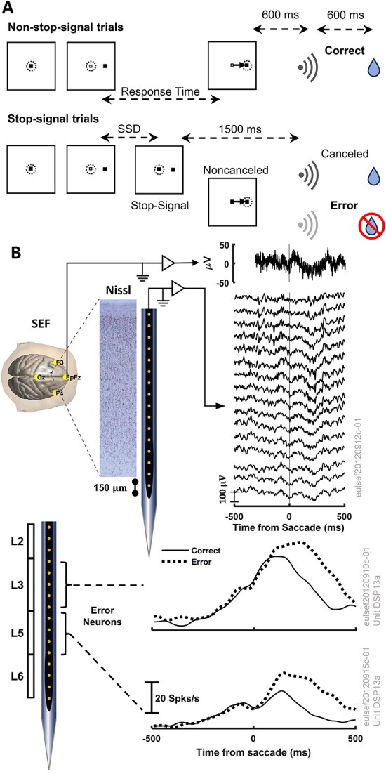
Experimental procedures and methodology. A. Stop-signal saccade countermanding task. All trials started with the presentation of a square fixation marker. Monkeys were required to hold fixation for a variable interval after which the center of the square was extinguished simultaneously with the presentation of a peripheral target on the right or left. On no-stop-signal trials, monkeys shifted their gaze to the target, whereupon after 600 ± 0 ms a high-pitched tone was delivered followed 600 ± 0 ms later by fluid reward. On stop-signal trials, a variable SSD after target presentation the center of the fixation spot was re-illuminated instructing the monkey to inhibit the planned saccade. If monkeys canceled the saccade, the high-pitch tone was presented after 1500 ± 0 followed 600 ± 0 ms later by fluid reward. SSD was adjusted such that monkeys successfully canceled the saccade in ~ 50% of the trials. If monkeys produced a noncanceled error, a low-pitch tone was presented 600 ± 0 ms after the saccade and no fluid reward was delivered. B. Schematic of concurrent EEG and LFP recording in SEF used to calculate theta power and CSD after saccades (top) and mean spike rate of representative L3 and L5 putative error PCs (bottom).

Cortical mapping and electrode placement

Chambers implanted over the medial frontal cortex were mapped using tungsten microelectrodes (2–4 MΩ, FHC, Bowdoin, ME) to apply 200 ms trains of biphasic micro-stimulation (333 Hz, 200 μs pulse width). The SEF was identified as the area from which saccades could be elicited using <50 μA of current (Schlag and Schlag-Rey 1987; Schall 1991). In both monkeys, the SEF chamber was placed over the left hemisphere. The dorsomedial location of the SEF makes it readily accessible for linear electrode array recordings across all cortical layers. A total of 5 penetrations were made into the cortex—2 in monkey Eu and 3 in monkey X. Three of these penetration locations were perpendicular to the cortex. In monkey Eu, the perpendicular penetrations sampled activity at site P1, located 5 mm lateral to the midline and 31 mm anterior to the interaural line. In monkey X, the perpendicular penetrations sampled activity at sites P2 and P3, located 5 mm lateral to the midline and 29 and 30 mm anterior to the interaural line, respectively. However, during the mapping of the bank of the cortical medial wall, we noted both monkeys had chambers placed ~ 1 mm to the right respective to the midline of the brain. This was confirmed through co-registered CT/MRI data. Subsequently, the stereotaxic estimate placed the electrodes at 4 mm lateral to the cortical midline opposed to the skull-based stereotaxic midline. A total of 16 perpendicular sessions were recorded across monkeys (Eu: 6 (Site P1), X: 6 (Site P2) and 4 (Site P3)).

Spiking activity and LFP recordings

During recordings, monkeys sat in enclosed primate chairs with heads restrained 45 cm from a CRT monitor (Dell P1130, background luminance of 0.10 , 70 Hz) subtending 46° × 36° of visual angle. Daily recording protocols were consistent across monkeys and sessions. After advancing the electrode array to the desired depth, electrodes were allowed to settle for 3–4 h to ensure stable recordings.

Spiking activity and LFPs were recorded from SEF using a 24-channel U probe (Plexon, Dallas, TX) with 150 inter-electrode distance. The U probes had 100 mm probe length with 30 mm reinforced tubing, 210 probe diameter, 30° tip angle, 500 to first contact. Contacts were referenced to the probe shaft and grounded to the metal headpost. All data were streamed to a data acquisition system (MAP, Plexon, Dallas, TX). Time stamps of trial events were recorded at 500 Hz. Eye position data were streamed to the Plexon computer at 1 kHz using an EyeLink 1000 infrared eye-tracking system (SR Research, Kanata, Ontario, Canada). LFP and spiking data were processed with unity-gain high-input impedance head stages (HST/32o25-36P-TR, Plexon).

LFP data were bandpass filtered at 0.2–300 Hz and amplified 1000 times with a Plexon preamplifier and digitized at 1 kHz. Neuronal spiking data were bandpass filtered between 100 Hz and 8 kHz and amplified 1000 times with a Plexon preamplifier, filtered in software with a 250 Hz high-pass filter, and amplified an additional 32,000 times. Waveforms were digitized from −200 to 1200 relative to threshold crossings at 40 kHz. Thresholds were typically set at 3.5 standard deviations from the mean. Single units were sorted online using a software window discriminator and refined offline using principal components analysis implemented in Plexon offline sorter.

Cortical depth and layer assignment

Depth alignment and laminar assignment were performed across sessions as described previously (Godlove et al. 2014). Briefly, flashed visual stimulation was delivered to the monkeys between sessions. Recording sessions were aligned relative to the initial visually evoked sink observed on the laminar CSD using an automated depth alignment algorithm. The procedure minimized the differences between the averaged visually evoked CSD across sessions in the 50–100 ms window after the visual stimulus onset. The minimum of the initial visually evoked sink, located in L3, was set as depth zero. Based on this convention, the algorithm identified depths 0.21, 0.36, and 1.02 mm as L1 to L2/3, L3 to L5, and L5 to L6 laminar boundaries, respectively.

Analysis of spiking activity

We examined activity in 2,386 trials (Monkey Eu: 1,608; Monkey X: 778) across 16 sessions in which the probe was verified to be perpendicular to the cortical layers. Trials were selected after response-time matching (Godlove et al. 2014; Ninomiya et al. 2015; Sajad et al. 2019). In these sessions, we isolated a total of 293 single units (Eu: 104, X: 189), of which 42 neurons (Eu: 39, X: 3) showed a greater discharge rate following erroneous (non-canceled) relative to correct saccades (Sajad et al. 2019). Two criteria have been used to define these differences: (i) if the difference in spiking rate between error and correct trials exceeded 6 standard deviations above the baseline, then it need to persist for only 50 ms, or (ii) the difference in spiking rate exceeded 2 standard deviations above a baseline difference measured during the 300 ms period before target onset and persisted for at least 100 ms.

The functional properties of these neurons, henceforth referred to as “error neurons,” were described previously (Stuphorn et al. 2000; Sajad et al. 2019). Error neurons were divided into putative PCs if their spike waveform had a peak-to-trough width >250 and interneurons if the width <250 (Sajad et al. 2019). In total, 37/42 error neurons had broad spike waveforms and were classified as putative PCs. Of these 37, 30 could be assigned to L3 (n = 18) and to L5 (n = 12) of monkey Eu. The only error PC found in monkey X was from L6 and was excluded from further analysis.

We used a combination of custom-written MATLAB functions (MATLAB 2021b, MathWorks) and the FieldTrip toolbox for performing the analyses (Oostenveld et al. 2011).

Single unit spike rate was estimated on a trial-by-trial basis by calculating the peri-stimulus time histogram (PSTH) of recorded spike trains and convolving them with a Gaussian of zero mean and 10 ms standard deviation. We utilized a bin size of 10 ms to calculate the PSTHs. Trials were defined from −500 to 1000 ms relative to saccade initiation time. The average instantaneous spike rate for each recorded unit was obtained by taking the mean across trials.

Only saccades from error and correct trials with similar reaction time (RT) (within 10 ms) and direction were used for comparison. We excluded from the analysis all error trials in which the stop-signal appeared after saccade initiation time. Trials with unstable spiking activity were also excluded from the analyses.

We characterized the spiking profiles of error neurons based on the patterns of successive ISI in the pre-target and the post-saccade periods. ISI distributions were calculated using the function ft_spike_isi() from the FieldTrip toolbox (Oostenveld et al. 2011) with a bin size of 2 ms. For calculating the pre-target ISI distributions, we considered all spikes produced from the beginning of the trial until target presentation. We calculated the pre-target ISI distribution for error and correct trials individually but found no differences. Thus, we combined all trial types for calculating the final pre-target ISI distribution. We obtained the post-saccade ISI distributions considering all spikes fired after saccade initiation and before the delivery of the feedback tone. ISI distributions were normalized by the total number of trials before calculating the averaged ISI distribution across neurons.

Analysis of LFPs

All analyses were done in MATLAB using custom-written scripts and the FieldTrip toolbox (Oostenveld et al. 2011). LFPs were epoched from −500 to 1,000 ms relative to the saccade initiation time, and low-pass filtered at 100 Hz using a 2-pass fourth-order Butterworth filter. Recorded trials were separated into correct no-stop-signal and error non-canceled trials. ERPs were time-locked to saccade initiation and baseline corrected to the 200 ms interval preceding the target onset (Godlove et al. 2014).

We computed the CSD from ERPs using the spline-iCSD method (Pettersen et al. 2006) as implemented in the CSDplotter toolbox (https://github.com/espenhgn/CSDplotter) with custom MATLAB (R2021b, The MathWorks) scripts (Herrera et al. 2020, 2022).

Frequency domain analysis

Time-varying laminar power maps per frequency band were calculated from the LFPs using the Hilbert transform. First, we bandpass filtered the raw LFPs before selecting the trials between 4–8 Hz (θ band), 9–14 Hz (alpha band), 15–29 Hz (beta band), and 30–80 Hz (gamma band). We constructed 4 Equiripple Bandpass FIR filters using Parks-McClellan optimal FIR filter design, as implemented in firpm() function from MATLAB’s Signal Processing Toolbox 6.14. The optimal filter orders were determined using firpmord() function. Supplemental Fig. S1A shows the magnitude response function of the designed filters. Second, we epoched the filtered LFPs from −500 to 1,000 ms relative to the saccade initiation time. Third, we calculated the Hilbert transform of the filtered LFPs per electrode contact for each trial. Next, we extracted the time-varying power estimates per electrode contact by taking the squared magnitude of the Hilbert transform of the filtered LFPs and then, baseline corrected them to the mean power in the 200 ms interval preceding the target onset. The final time-varying laminar LFP power maps were obtained by taking the mean across the single trial laminar power estimates. Supplemental Fig. S1A illustrates the filtering and epoching procedures and Supplemental Fig. S1B the trial-level processing steps followed to calculate the single trial laminar LFP power estimates.

Biophysical modeling

PC models

We simulated the spiking activity of L3 PCs using the previously described model by Eyal et al. (2018) (ModelDB, accession #238347, 2013_03_06_cell03_789_H41_03, active model cell0603_08_model_602). L5 PCs were modeled as previously described in Hay et al. (2011) (ModelDB, accession #139653, “cell #1”), incorporating the modifications of voltage-gated calcium channel densities as in Shai et al. (2015) and Ih channel density distribution as in Labarrera et al. (2018) and Leleo and Segev (2021). Using this modified version of Hay et al. (2011), Leleo and Segev (2021) model allowed us to decrease the bursting activity of the neuron and obtain ISI distributions closer to those observed in the experimental data.

Synaptic inputs

For all simulations, unless otherwise specified, we considered modeled neurons that received excitatory NMDA and AMPA synaptic inputs randomly distributed along their dendrites in clusters of 20 synapses within 20 (Yadav et al. 2012; Kastellakis et al. 2015). The location of the synapses varied for each simulated neuron and trial. The number of NMDA and AMPA synapses for each neuron type was set based on the approximate density of NMDA and AMPA receptors in SEF (area F7d) of macaque monkeys reported in the literature (Geyer et al. 1998; Rapan et al. 2021). We considered the total number of NMDA synapses in the oblique and basal dendrites of L5 PCs (890 synapses) as a reference and determined the number of NMDA synapses in the distal apical dendrites of these neurons based on the relative density of NMDA receptors across the neuron. The total number of AMPA synapses across a simulated L5 PC was calculated based on the ratio of NMDA and AMPA synapses (AMPA-NMDA ratio: 0.1045) (Rapan et al. 2021). Similarly, we estimated the number of AMPA and NMDA synapses on simulated L3 PCs relative to the set number of NMDA synapses on simulated L5 PCs considering the ratio of L3 to L5-distal-apical AMPA (0.59) (Datta et al. 2015). In summary, we considered a total of 1080, 600, and 1200 NMDA synapses along the basal, oblique, and distal apical dendrites of L3 PCs, and 100, 60, and 120 AMPA synapses, respectively. For L5 PCs, we considered 580 and 444 basal and distal apical dendritic NMDA synapses, and 60 and 132 AMPA synapses, respectively.

AMPA- based synaptic currents were modeled as (Eyal et al. 2018): ; with , and . NMDA-based synaptic currents were modeled according to the standard formalism (Jahr and Stevens 1990): , ; ; with representing the voltage-dependent magnesium (Mg) block. The equations for and are given by (Eyal et al. 2018): with and . and (Eyal et al. 2018), and and (Jahr and Stevens 1990). For each synapse model, represents the post-synaptic membrane potential, and the onset time of the presynaptic spike. , , and are the synaptic reversal potential, the gating variable representing the proportion of open channels, and the maximum synaptic conductance, respectively.

Estimation of synaptic inputs activation profiles from observed data

We simulated background excitatory inputs onto L3 and L5 PCs by randomly activating the excitatory synapses on the PC models following a Poisson distribution with a fixed mean. We manually adjusted the mean of the Poisson process to replicate the observed averaged ISI distribution and spike rate of recorded L3 and L5 putative error PCs during the pre-target period. To keep consistency in our model fitting, we included only error PCs satisfying criterion (1) in their spiking rate profiles, i.e. if the difference in spiking rate between error and correct trials exceeded 6 standard deviations above the baseline, then it need persist for only 50 ms (see Analysis of Spiking Activity). Therefore, from the total number of error PCs (n = 30), we used 10 from L3 and 5 from L5 for the final calculations of the averaged ISI distribution and spike rate.

We modeled time-locked saccade-related inputs as spike generators with a predefined temporal profile relative to the saccade onset time. On a trial-by-trial basis, presynaptic spike times were chosen from a skew-normal distribution (Jones et al. 2007). The number of pre-synaptic temporal profiles and their location along the neuron, as well as their skewness, mean, and standard deviation, were estimated to reproduce the spiking activity and ISI distribution of recorded L3 and L5 putative error PCs relative to saccade onset.

To account for the variable target times and RT observed in the experimental data, we calculated the distribution of target times and saccade times from the experimental data and used these distributions to randomly generate target and saccade onset times for each simulated trial.

Analysis of simulated spiking activity

Simulated ISI distributions and spike rates were calculated following the same methodology as for the experimental data. To mimic some of the variability observed in the recorded neurons, we simulated the same number of selected putative L3 (n = 10) and L5 (n = 5) error PCs and a total of 106 trials, the mean number of trials across sessions in the experimental recordings. In each of these simulations, we randomly varied the location of the pre-synaptic inputs on the modeled neurons while keeping constant the total number of NMDA and AMPA synapses. Spike times were obtained from the simulated somatic membrane potentials using the peak_detection() function of the Elephant Python package (Denker et al. 2018) with a threshold of 0 mV. To calculate the post-saccade ISI distributions of simulated neurons, we randomly generated the delivery time of the feedback tone for each simulated trial from the experimental distribution of tone times. As for the experimental data, we excluded all spikes fired after the tone.

Analysis of simulated field potentials

We studied the contribution of L3 and L5 error PCs to the extracellular field potentials by simulating the activity evoked by a population of unconnected L3 and L5 error PCs under the estimated synaptic inputs. There are approximately 40,000 neurons per in SEF—cytoarchitecturally defined as area F7 of macaque monkeys (Turner et al. 2016). We have shown that 18% and 16% of the neurons recorded from L3 and L5, respectively, are error neurons (Sajad et al. 2019, 2022), and that ~ 90% of them are putative PCs. Based on previous data collected by our group (Schall 1991; Stuphorn et al. 2010; Godlove et al. 2014) to determine the extent of SEF in macaques, we estimated that a cylindrical cortical column of 3 mm diameter representing SEF would have at least 17,177 L3 and 27,483 L5 error PCs (Turner et al. 2016), yielding a ratio of L5-to-L3 error PCs of 1.6. Simulations were accomplished using high-performance computing at Vanderbilt University (https://www.vanderbilt.edu/accre/). Simulating an unconnected network of 17,177 (L3) and 27,483 (L5) error PCs for multiple trials in both conditions (error and correct trials) was prohibitive, so to reduce the computational costs, we simulated the activity evoked by a reduced population of 625 L3 and 1,000 L5 PCs, keeping the 1.6 ratio of L5-to-L3 error PCs. Because summation of current is linear, the magnitude of the laminar CSD obtained from the simulated LFPs was multiplied by a factor of 27.48 (44,660 estimated error PCs divided by 1,625 simulated error PCs).

We calculated the LFP produced by the activity of the neurons at 16 equally spaced vertically aligned points located at the center of the 3 mm diameter cortical column. As in the experiments, the inter-electrode distance was 150 μm. The soma of the neurons was randomly located within the cylindrical cortical column in their associated cortical layers, with height corresponding to the vertical extent in area SEF of lower L3 (700–1,100 below the pia matter) and L5 (1,125–1,750 ). LFPs were calculated from the transmembrane currents using the point-source approximation in LFPy (Lindén et al. 2014; Hagen et al. 2018). The point-source approximation assumes that each transmembrane current can be represented as a discrete point in space, the center of each neuronal compartment. Considering the extracellular medium is homogeneous and isotropic with an extracellular conductivity , the extracellular potential at the electrode can be calculated by

(1)

where , , and denote the total number of distinct neuron populations, the number of neurons in the p-th population, and the number of compartments in the i-th neuron of the p-th population, respectively. indicates the coordinates of the -th compartment of the -th neuron in the -th population and the coordinates of the electrodes. is the transmembrane current of the -th compartment of the -th neuron in the -th population.

The LFP was obtained by low pass filtering the extracellular potentials () at 100 Hz. LFPs were baseline corrected to the 200 ms interval preceding the target onset. The CSD patterns of the synthetic data sets were calculated using the spline-iCSD method (Pettersen et al. 2006) with the custom MATLAB (R2021b, The MathWorks) scripts used for the experimental data (Herrera et al. 2020, 2022). We obtained the time-varying laminar power maps per frequency band from the simulated LFPs using the same analysis pipeline as for the experimental data (Supplemental Fig. S1).

Simulations

All biophysical simulations were performed in Python using NEURON 8.0 (Hines et al. 2009) and LFPy 2.2 (Hagen et al. 2018). Data analysis was performed in MATLAB (R2021b, The MathWorks).

E‌EG forward model

To calculate the EEG potential at the position of the electrodes (Fig. 7A), we modeled the monkey’s head as an isotropic and piecewise homogenous volume conductor comprised of the scalp, inner and outer skull, and the cortex surface. For both the experimental and simulated data, we utilized a volume conductor model of the monkey’s head constructed in Brainstorm (Tadel et al. 2011) from the symmetric surfaces provided in the NIMH Macaque Template version 2.0 (Jung et al. 2021) (Fig. 7A). The scalp, skull, and brain conductivities were set as 0.43, 0.0063, and 0.33 S/m (Lee et al. 2015), respectively. In the experimental recordings, only electrodes FpFz, Cz, F3, and F4 were used. Thus, we considered the same electrode positions for our EEG calculations. We obtained the position of the electrodes on the scalp surface of the NIMH Macaque Template using the algorithm from Giacometti et al. (2014) for the EEG 10–10 system.

Fig. 7.

Multipole moments derived from observed (left) and simulated (right) CSD. A. Left—volume conductor model of the monkey’s head (BEM) with surfaces color-coded and electrodes represented by yellow discs. Surfaces for constructing the BEM model of the monkey’s head were obtained from the NIMH macaque template version 2.0 (Jung et al. 2021). Right—location of the SEF current sources used in the EEG forward model. B-C. The time course of the monopole (m_z, top), dipole (d_z, middle), and quadrupole (q_z, bottom) moments are plotted for correct (thin solid) and error (thick dotted) trials and their difference (magenta, thick solid). The time of peak polarization of ERN (dash) and Pe (dot–dash) are indicated. The unbalanced current observed across depths creates the monopole moment. The simulated dipolar and quadrupolar moments were 3 orders of magnitude weaker than the observed. Scaling up multipoles by increasing the density of error PCs was not enough to reproduce the temporal profiles of these LFP and scalp potentials.

The EEG potential at the electrode position evoked by a continuous field of microscopic electric currents inside the brain can be calculated by equation (2) (Riera et al. 2012; Herrera et al. 2022):

(2a)

(2b)

(2c)

with representing the secondary currents defined for each elemental volumetric shell (i.e. a surface of thickness ). and denote the conductivity and surface potential of the k-th compartment in the head model (i.e. brain (), skull, and scalp)., and the normal vector to the surface () of the k-th compartment at the location . Considering that for and otherwise, where V is the volume of the brain region of interest SEF, centered at ; and the location of the EEG electrodes () is far enough from the center , then can be calculated as a function of the multipolar moments (Riera et al. 2012). Under this assumption, the EEG forward model can be represented by equation (2a) and the following equation for (Riera et al. 2012):

(3)

with ; ; and . is the gradient operator with respect to . The notation and denote the scalar product of 2 vectors and the full contraction of 2 second-rank tensors, respectively. Their definitions can be found in (Jerbi et al. 2002).

The first, second, and third terms in equation (3) represent the contribution of the current monopole, dipole, and quadrupole, etc., to the EEG, respectively. We demonstrated in Herrera et al. (2022) that the activity of a cortical column can be accurately represented by a single equivalent dipole at the center of the column, whose orientation corresponds to that of the cortical surface and whose temporal dynamic is obtained from the laminar CSD. Using this approach, we calculated the first 3 current multipole moments from the experimental and simulated CSDs using the following equations:

(4)

(5)

(6)

Because of the electroneutrality principle in neural tissue, theoretically the current monopole contribution (equation (4)) should be zero (Nunez and Srinivasan 2006). However, estimated CSDs from intracranial recordings are not always balanced along the cortical column, i.e. the total estimated current within the cortical column does not sum to zero. We discuss possible causes for this unbalanced current later in the Discussion. Thus, we imposed a monopole and quadrupole moment at the center of the column, at the same location as the equivalent current dipole, to compensate for the current imbalance. This was the case for the observed CSD that had no-zero monopole contribution. The simulated CSD had zero monopole contribution, as expected since the transmembrane currents of compartment models sum to zero at all times. Estimated EEGs were calculated considering there were 2 symmetric brain sources in SEF, one in each hemisphere. For computing the EEG dipolar contribution, we assumed the orientation of the dipoles corresponded to that of the cortical surface at the dipoles’ location.

Quantification and statistical analysis

Spiking activity

We used non-parametric permutation tests to compare the spike rate features (peak amplitude, peak latency, and peak half-width) between observed and simulated neurons. We used a 2-tailed paired t-test to calculate the permutation test statistic and the Monte Carlo method (100,000 permutations for L3 neurons and all possible (40,320) permutations for L5 neurons) for calculating the significance probability, an estimate of the P value under the permutation distribution. The P values were reported in the main text or figure captions. The amplitude, latency, and half-width of the peak in the spike rates after the saccade were calculated using the findpeaks() function from MATLAB’s Signal Processing Toolbox.

Laminar time-varying field potential frequency power maps

We compared the averaged time-varying laminar power maps of error versus correct trials across sessions (16 sessions, Eu: 6 and X:10) for each frequency band employing nonparametric clustered-based permutation tests (Maris and Oostenveld 2007). We used a 2-tailed paired t-test to contrast error versus correct trial averages at the sample level (channel-time-pair samples). Un-smooth power maps were used for the statistical tests. All pairs with t-statistics larger than the critical threshold () were clustered in connected sets based on spatial and temporal adjacency. The cluster-level statistic was calculated by taking the sum of the sample-specific t-statistics within each cluster, and the permutation test statistic was defined as the maximum of the cluster-level test statistic. We utilized the Monte Carlo method for calculating the significance probability, an estimate of the P value under the permutation distribution. We considered the maximum number of unique permutations for comparison across sessions from each monkey. Significant clusters were determined by comparing their Monte Carlo P value with an overall 2-tailed critical threshold, ( for each tail).

For comparing the simulated error and correct trials, we also employed a nonparametric permutation test but considered a 2-tailed unpaired t-test for the sample level statistic (10,000 permutations). In contrast to the experimental data in which we have 2 experimental conditions per session, only one experimental condition is assigned to each simulated LFP (between-trial analysis) (Maris and Oostenveld 2007).

Results

Electrophysiological recordings

Concurrent scalp EEG and laminar recordings of spiking activity and LFPs were obtained in the SEF of 2 monkeys (Godlove et al. 2014; Ninomiya et al. 2015) performing the saccade countermanding stop-signal task (Hanes and Schall 1995) (Fig. 1). Briefly, monkeys were required to generate a saccade to a peripheral target, but to inhibit this planned saccade when a stop-signal appeared. Errors occurred when monkeys generated a saccade despite the appearance of the stop-signal. Monkeys produced response errors similar to human participants and demonstrated homologous ERN features (Godlove, Emeric, et al. 2011a; Reinhart et al. 2012).

Reproducing the spiking activity of L3 and L5 error putative PCs

To evaluate the role of error PCs in the midfrontal theta and ERN generation, we first reproduced their spiking activity using detailed biophysical neuronal models. Most of the putative error PCs were recorded from L3 and L5 (30/37) (See (Godlove et al. 2014) and (Sajad et al. 2019) for these methods). Compared with those recorded from L6, they showed a similar spiking profile relative to saccade onset across neurons. Thus, we focused on modeling the activity of these 2 populations of neurons. We employed a model-optimization approach to estimate the excitatory pre-synaptic inputs received by these neurons around saccade onset. We described the activity of L3 error PCs using the model proposed by Eyal et al. (2018). L5 error PCs were described using the Hay et al. (2011) model, including modifications of voltage-gated calcium channel densities as in Shai et al. (2015) and hyperpolarization-activated cyclic nucleotide—HCN or Ih—channel density distribution as in Labarrera et al. (2018). The simulations included only excitatory NMDA and AMPA synaptic inputs with distributions and ratios corresponding to those in area F7d (SEF) estimated from the literature (Geyer et al. 1998; Rapan et al. 2021). The total number of NMDA and AMPA synapses per type was fixed for each simulated neuron, but their location was randomly selected in each neuron and simulation (Fig. 2A, 3A). Non-specific background pre-synaptic inputs were Poisson processes with a fixed mean (Fig. 2B, 3B).

Fig. 2.

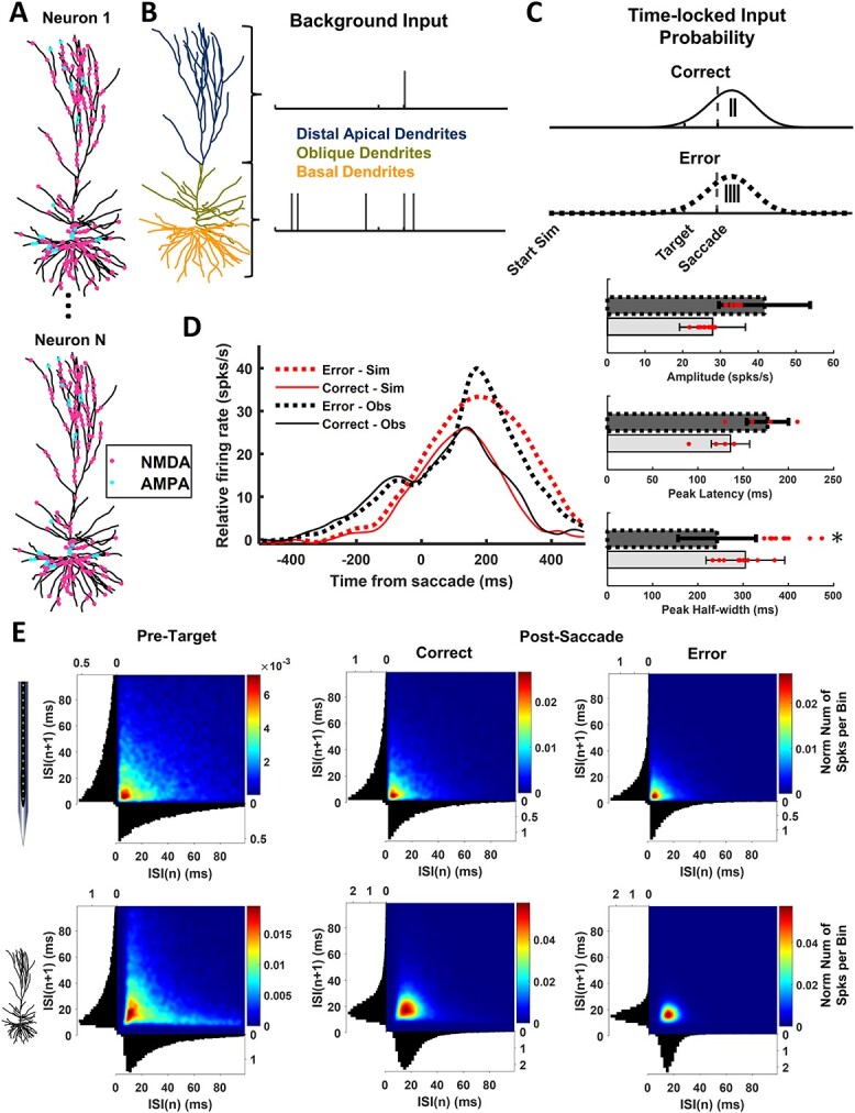
Simulation of L3 error PCs optimized to replicate observed discharge rates and ISIs. A. Representative randomized locations of NMDA and AMPA synapses on simulated L3 PC (ModelDB, accession #238347, 2013_03_06_cell03_789_H41_03, active model cell0603_08_model_602). B. Observed baseline spiking statistics were replicated by activating NMDA and AMPA synapses located on the distal apical, basal, and oblique dendrites. The timing of pre-synaptic inputs was drawn from Poisson distributions with a mean of 2 for basal and oblique dendritic synapses and a mean of 3.5 for distal apical synapses. C. Spiking statistics after saccade initiation were simulated by activating distal apical and basal synapses with spike times drawn from a left-skewed normal probability distribution (skewness = −1). To replicate observed post-saccadic error-related modulation, for correct trials 2 spikes were drawn from a distribution with a mean of 216.6 ms and a standard deviation of 141.6 ms, and for error trials 4 spikes, from a distribution with a mean of 298.6 ms and a standard deviation of 178.6 ms. The vertical lines indicate the total number of pre-synaptic spikes that each synapse will receive under its associated probability distribution. D. Observed (black) and simulated (red) mean spike rate for correct (thin solid) and error (thick dotted) trials (left) with comparisons of observed (bars) and simulated (dots) peak amplitude, peak latency, and peak half-width (right). Based on non-parametric permutation tests the simulated values were not different from observed amplitude (correct trials, P = 0.5107; error, P = 0.0654), peak latency (correct, P = 0.2449; error, P = 0.5449), and peak half width for correct (P = 0.1083) but not error trials (P = 0.00036). E. Observed (top) and simulated (bottom) ISI_n + 1 versus ISI_n with heatmap indicating the normalized number of spikes count per bin and marginal distributions before target presentation (left) and after correct (middle) and error (right) saccades. Simulated ISI produced the observed bursting pattern of successive ISI.

Fig. 3.

Simulation of L5 error PCs optimized to replicate observed discharge rates and ISIs. Conventions as in Fig. 2. A. Representative randomized locations of NMDA and AMPA synapses on simulated L5 PC (ModelDB, accession #139653, “cell #1”). B. Observed baseline spiking statistics were replicated by activating NMDA and AMPA synapses on the basal dendrites with input times drawn from Poisson distributions with a mean of 2. C. Spiking statistics before all saccades were simulated by activating basal synapses with 2 pre-synaptic spike times drawn from a normal distribution (σ = 140 ms) centered 70 ms before saccade initiation. Spiking statistics after correct saccades were simulated with inputs to distal apical dendrites drawn from a right-skewed normal distribution (skewness = 2, σ = 200 ms) centered 100 ms after the saccade plus a basal dendritic input drawn from a right-skewed normal distribution (skewness = 5, σ = 250 ms) centered 120 ms after the saccade. Spiking statistics after error saccades were simulated by distal apical inputs with the same probability distribution as in correct trials plus a basal input at 120 ms with the same probability distribution as in correct trials sufficient to yield 5 pre-synaptic spikes and a second distal apical input drawn from a right-skewed normal distribution (skewness = 5, σ = 250 ms) centered 280 ms after the saccade. D. Simulated values were not different from observed amplitude (correct trials, P = 0.4841; error, P = 0.4188), peak latency (correct, P = 0.3783; error, P = 1.0000), and peak half width (correct, P = 0.1553; error, P = 0.3669). E. Simulated ISI produced the observed shorter ISI during error trials.

We determined the mean of the Poisson process that replicated the observed mean ISI distribution and spike rate of observed error PCs during the pre-target period. Inputs synchronized on saccade production were modeled as spike generators with specified temporal profiles. On a trial-by-trial basis, pre-synaptic spike times were chosen from a skewed-normal distribution (Jones et al. 2007). The number of pre-synaptic spikes and their location along the neuron, as well as their skewness, mean, and standard deviation, were optimized to reproduce the observed spiking activity of L3 and L5 error PCs.

The ISI distribution of L3 putative error PCs during the pre-target and post-saccade period followed an exponential function (Fig. 2E). In contrast, L5 putative error PCs had a uniform ISI distribution during the pre-target interval and a double exponential distribution during the post-saccade period (Fig. 3E). Additionally, L5 error PCs exhibited more bursts after errors compared with correct trials.

To estimate the background inputs to the neurons, we distinguished 3 groups of synaptic inputs according to their dendritic location—basal, oblique, and distal apical (Fig. 2A, 3A). This distinction was also used for optimizing the inputs before and after the saccade. We assumed all synapses belonging to each of these groups were activated by a Poisson process with the same mean. We simulated the spiking activity of L3 error PCs using a Poisson process with a mean equal to 3.5 for synapses located in the basal and oblique dendrites and 2.0 for synapses located in the oblique dendrites and distal apical dendrites. Figure 2B illustrates the synaptic activation profile of a representative background input coming to the basal and oblique dendrites and the distal apical dendrites using the estimated mean of the Poisson processes. Figure 2E shows the ISI distribution of the simulated neurons before target presentation and after the saccade for correct and error trials, respectively. The optimized biophysical models replicated the observed bursting activity (Fig. 2E). However, the minimum ISI and the normalized number of spikes count per ISI bin were larger than those observed in the experimental data. We believe this is because simulated L3 PCs could not produce ISIs smaller than 5 ms.

To reproduce the baseline activity of L5 error PCs, we only activated basal dendritic synapses with a Poisson process with a mean equal to 2.0 (Fig. 3B). Activation of either oblique or distal apical synapses resulted in an increase of bursting activity that was not present in the observed data during the pre-target period (Fig. 3E). While we replicated the mean spike rate of the observed L5 error PCs (Fig. 3D), the simulated ISI distributions favored ISI around 20 ms and did not show a uniform distribution (Fig. 3E). We believe the differences in the ISI distributions of observed and simulated error neurons are attributable to differences in the biophysics of the neuronal models used and variability in the biophysics of recorded neurons, not being captured by the model (see Discussion).

After optimizing the background inputs of the models, we optimized the temporal profile, location, and sequence of time-locked inputs influencing the neuron after the execution of a correct or error saccades. We calculated the mean spike rate of recorded L3 and L5 putative error PCs during the interval from 500 before to 500 ms after saccade initiation (Fig. 2D, 3D). The observed spike rate of error PCs in L3 and L5 peaked after the execution of a saccade and slowly returned to a pre-saccadic spike rate with the pre-saccadic spike rate exceeding the pre-target firing in L5 error PCs.

To evaluate the quality of the optimization, we quantified the mean amplitude, latency, and half-width of the peak (Fig. 2D, 3D). To fit these parameters, we manually optimized the time-locked inputs for the simulated neurons. The observed spiking activity of L3 error PCs was replicated by activating half of all the synapses with the same probability distribution and increasing the number of pre-synaptic spikes in error compared with correct trials (Fig. 2C). Conversely, simulated L5 error PCs were sensitive to both the location and temporal profile of pre-synaptic inputs as well as to the number of pre-synaptic spikes. Activation of oblique dendrite synapses facilitated bursting resulting in an exponential, rather than double-exponential, post-saccade ISI distribution. Thus, our final optimization of time-locked inputs only used basal and distal apical synapses (Fig. 3C).

To replicate the activity of L5 error PCs (Fig. 3D), we needed an initial basal input 70 ms before the saccade in both trial types (normal distribution: , , 2 pre-synaptic spikes) followed by a distal apical input 100 ms after the saccade (skewed normal distribution: , , ) and another basal input 120 ms after the saccade (right skewed normal distribution: , , ) (Fig. 3C). After the saccade on correct trials, all basal dendrite synapses had a probability of receiving 2 pre-synaptic spikes, and all distal apical synapses had a probability of receiving 1 pre-synaptic spike (Fig. 3C). On error trials, we needed more pre-synaptic spikes (5) coming to the second basal input around 120 ms after the saccade and a second distal apical input of 1 spike arriving 280 ms after the saccade (right skewed normal distribution: , , ) (Fig. 3C). The increase in sustained firing after saccades observed in L5 error PCs was produced by increasing the mean of the Poisson process for the basal background inputs from 2 to 4 after the saccade. As in the simulations of L3 error PCs, only half of the synapses received the time-locked inputs. Figure 3E shows the observed and simulated ISI distributions of L5 error PCs in the post-saccade period. In summary, we replicated the spike rate profiles of error PCs and qualitatively explained their ISI distributions during both the pre-target and post-saccade periods (Figs. 2 and 3).

Error PCs drive midfrontal theta

Midfrontal theta is a prominent signature of performance monitoring in human EEG studies (Cavanagh and Frank 2014; Cohen 2014), being elevated on error compared with correct trials. Yet, the cellular mechanisms generating this signal are unknown. Here, we characterized the presence of theta oscillations in SEF and used biophysical modeling to ascertain whether error PCs in SEF can produce such a rhythm. First, we measured the laminar profiles of theta (θ) as well as alpha (α), beta (β), and gamma (γ) power after correct and error saccades. We compared modeling results with sampled data. Across sessions, we observed a 30%–74% increase in theta power after correct saccades and a 30%–122% increase after error saccades (Fig. 4, top panels). This increase in theta power was significantly larger on error versus correct trials (nonparametric clustered-based permutation test, n = 6, P < 0.01), extending from L3 to deep layers. Maximal θ power was observed just before the peak polarization of the ERN (Sajad et al. 2019). These results were consistent across monkeys (Supplemental Fig. S2). We also observed significantly greater α, β, and γ power on error trials in Monkey Eu but not in Monkey X (Supplemental Fig. S2). The increase was observed in the β and γ bands well after the saccade and in the α band after the saccade with a magnitude half that observed for the θ band (Supplemental Fig. S2).

Fig. 4.

EEG and LFP θ power. The top row illustrates the average ERP obtained from electrode FpFz aligned on saccade on correct (left) and error (middle) trials with the resulting difference wave (right). The spike potential associated with saccade production is evident in the correct and error plots. The difference wave highlights the ERN followed by the Pe component. The next rows plot observed (middle) and simulated (bottom) average θ power across sessions through time across the cortical layers on correct and error trials with the time-depth difference. Colormap plots power modulation relative to the mean power during 200 ms before target presentation (μV²) for observed and simulated power. The time of peak polarization of ERN (dash) and Pe (dot–dash) are indicated. Statistically significant regions are outlined in the difference plot.

To assess the contribution of individual error PCs to the observed increase in the laminar theta power, we simulated the activity of 625 L3 and 1,000 L5 PCs activated by random samples from the range of inputs optimized to replicate the error-related modulation and the ISI. Neuron somas were randomly positioned in L3 and L5 in a cylindrical cortical column of 3 mm diameter, with height corresponding to the vertical extent in area SEF of L3 (700–1,100 below the pia matter) and L5 (1,125–1,750 below the pia matter). We calculated the LFP evoked by the activity of the simulated ensembles of error neurons at 16 equally spaced (150 μm) vertically aligned points in the center of the cortical column. Finally, to account for summation over a plausible estimate of the number of neurons in a column of SEF, we multiplied the LFPs in all channels by the 27.48 factor. Then, we compared the observed and simulated grand average laminar LFP and CSD in correct and error trials and their differences (Fig. 5). Individual session CSDs for each monkey and recording locations are shown in the supplementary material (Supplemental Fig. S3A). Supplemental Fig. S3B shows the individual contribution of L3 and L5 error PCs to the CSD for monkey Eu. Note that the simulated CSDs are an order of magnitude smaller than the experimental observations. On the other hand, the simulated LFPs are larger than the experimental. These results suggest the existence of missing microcircuit components in our simulations. Such missing elements include, for example, the PCs that do not signal errors as well as interneurons. The strong possibility of other current sources in SEF is counterbalancing the overall contribution of error PCs to the LFPs.

Fig. 5.

Observed (top) and simulated (bottom) average LFP and CSD. Simulated LFPs were evoked by the activity of 625 L3 and 1,000 L5 error PCs located in a cylindrical cortical column of 3 mm diameter and multiplied by a factor of 27.48 to account for the actual number of error PCs in SEF (see “Materials and Methods”—Analysis of simulated field potentials). Neither observed nor simulated CSD had a simple bipolar structure, but the simulated CSD did not replicate the observed CSD.

The observed laminar CSDs do not resemble a simple dipolar distribution, unlike observations in visual areas V1 (Mehta et al. 2000; Maier et al. 2011) or V4 (Herrera et al. 2022). Instead, the observed laminar CSD associated with both correct and error saccades consisted of 3 prominent sinks, one at the L3-L5 border, another in L5, and the third in deep L6. These were accompanied by a sequence of weaker, transient sinks in upper L3. Likewise, the CSD derived from the L3 and L5 error PCs simulations consisted of 3 sinks, 2 in L3 and 1 in L5. The simulated laminar CSD accounted for only ~ 3% of the observed laminar CSD.

Following the same analysis pipeline, we calculated the laminar profiles of θ power relative to saccade initiation on the simulated LFPs in both correct and error trials (Fig. 4, bottom panels). The simulations predicted that L3 and L5 error PCs alone would evoke an increase in power with post-saccadic time lags similar to those observed experimentally in both conditions. Note that this increase is sharply terminated at the time of the ERN peak. More importantly, as in the experimental data, simulated LFPs showed a significantly greater increase in post-saccadic θ power on error versus correct trials (nonparametric clustered-based permutation test, n = 20, P < 0.01). However, the increase in power was 3 times the observed value. As mentioned before, these predictions only account for the contribution of error PCs, which constitute ~ 6% of SEF neurons, and did not consider the contributions of other PCs and of interneurons. These populations of neurons might elicit oscillations that are not synchronized with the ones triggered by error PCs, decreasing the magnitude of the laminar θ power. We believe a complete microcircuit model of SEF would explain the observed relative laminar θ power. Analysis of the contribution of the individual populations of L3 and L5 simulated error PCs indicate that L5 error PCs, but not L3 error PCs, produce the increase in θ power around saccade. These results indicate that L5 error PCs contribute to the observed laminar θ power but, unexpectedly, contribute little to the laminar current sources observed in SEF. Additionally, the simulated L3 and L5 error PCs did not produce the laminar profile observed in the other frequency bands, suggesting these signals might be generated from other circuit mechanisms (data not shown).

To explore whether these results were associated with the intrinsic properties of the neurons, we simulated the activity of 100 unconnected L3 and L5 PCs receiving randomly activated synaptic inputs. We looked at the spectral properties of their membrane potentials and evoked LFPs in the absence and presence of the synchronized activation of all synapses 1 s after the beginning of the simulation. The voltage response of simulated L3 and L5 PCs produced by the random input is shown in Supplemental Fig. S4. The power spectrum of the membrane potential of all L5 PCs but not L3 showed peaks in the low frequencies (θ and α bands) (Fig. 6). Inspection of the membrane potential θ phase revealed a phase-rest across L5 PCs for both dendritic and somatic membrane potential (Fig. 6B). In contrast, L3 PCs showed a phase-rest in their dendritic membrane potential, but not in their somatic membrane potential (Fig. 6A). Laminar LFP θ power maps showed an increase in θ power only for simulated L5 PCs under time-locked synchronized inputs (Fig. 6). These results indicate that L5 PCs can act as pacemakers of θ oscillations, but they are masked in the LFP unless the neurons receive a synchronized input to reset their phases.

Fig. 6.

Intrinsic rhythmicity of 100 simulated L3 (A) and L5 (B) error neurons with randomized distributions of AMPA (cyan) and NMDA (pink) synapses (left) activated randomly according to Poisson processes (L3: Basal mean = 2; apical mean = 1; L5: Basal mean = 5, oblique mean = 4, apical mean = 1) without (left) and with (right) a synchronized input at time zero. The mean power spectra () of somatic (salmon) and dendritic (light blue) membrane potentials (first row) illustrate the consistency of simulated neurons and pronounced peak in θ power in L5 but not L3 PCs. θ phase of the dendritic (second row) and somatic (third row) membrane potentials illustrate phase resetting of dendritic and soma membrane potentials of L5 neurons but only the dendritic potentials of L3 neurons. To quantify the laminar structure of θ power, the somas of the simulated neurons were randomly distributed within a cylindrical cortical column of 3 mm diameter with random depths within their associated cortical layers (L3 700–1,100 μm below the pia matter; L5 1,125–1,750 μm). The laminar distribution of LFP θ power (bottom row) demonstrates elevated θ power derived only from L5 PCs synchronized on the phase resetting.

Negligible contribution of error neurons to ERN current sources

Next, we employed EEG forward modeling to study SEF contributions to the ERN. We considered 2 current sources located in SEF symmetrically in each hemisphere (Fig. 7A). These current sources could comprise multipolar contributions: monopolar, dipolar, and quadripolar. The temporal dynamics of the multipolar components were calculated from the observed and simulated (scaled) laminar CSDs using the method proposed in our previous study (Herrera et al. 2022). Figure 7B-C shows the multipole moments in SEF obtained from the observed CSD and the CSDs generated by error PCs. The monopole moment of the simulated CSDs was by definition zero. In agreement with the previous results, even summing over the approximate number of error PCs in SEF, the dipole and quadrupole produced by the simulated error PCs were 3 orders of magnitude smaller than those observed in SEF. They also had different temporal dynamics. For clarity, we directly compared dipoles and quadrupoles for the error-minus-correct condition in Supplemental Fig. S5. Surprisingly, these results indicate a very weak and indirect biophysical contribution of the error PCs in SEF to the ERN. They, however, are not unexpected from a theoretical perspective because error PCs represent only ~ 6% of the total number of neurons in SEF. Future simulations incorporating other populations of neurons in SEF and the circuit dynamics are needed to test this hypothesis.

The scalp EEG at the FpFz electrode is shown in Fig. 8A. Figure 8B illustrates the forward model prediction of the scalp EEG at this electrode from each multipolar moment obtained from the observed CSDs in SEF. Note that the monopolar contribution was 1,000 times larger than the dipolar and quadrupolar contributions, with the latter two having nearly equivalent magnitudes. Finding a non-zero monopole contribution was caused by an unbalanced CSD across depth (see Discussion), a phenomenon previously reported in the somatosensory cortex of rats (Riera et al. 2012). In the absence of unbalanced current density, dipoles obtained from the observed CSD might explain better the EEG signal as previously reported for V4 (Herrera et al. 2022). However, as discussed below, the existence of monopolar sources might strongly affect EEG signal prediction as in the case of SEF. The resulting monopolar source was placed at the center of the SEF cortical column in both hemispheres. The dynamics of the dipolar moments paralleled the ERN. In contrast, the dynamics of the quadrupolar component coincided with the Pe. After normalizing EEG signals, the EEG predicted from the combination of all CSD multipole moments in SEF paralleled the dynamics of the ERN and Pe (Fig. 8C). However, the predicted scalp voltage at the ERN peak (black dashed line, Fig. 8A) was −0.60 μV, half an order of magnitude smaller than that observed experimentally (−2.43 μV). As for the Pe peak (blue dashed line, Fig. 8A), the predicted scalp potential (−1.00 μV) was substantially different from that experimentally observed (8.74 μV), including reverse sign.

Fig. 8.

Contributions of SEF to the ERN and Pe.. A. Cranial EEG during correct (thin solid) and error (thick dotted) trials with their difference (bottom panel) illustrating the ERN and Pe components. B. Comparison of the difference waves of the observed EEG (black, left axis) with the predicted EEG monopolar (top), dipolar (middle), and quadrupolar (bottom) components (red, right axis), respectively. The predicted EEG dipolar component explained ERN features and the quadrupolar component reproduced those for the Pe. The presence of a monopole might indicate strong electro-diffusion, dendritic/axonal electrotonic current leakage outside SEF, or violations of the model assumptions (see Discussion). C. Comparison of EEG observed (black) and predicted (red) from the multipolar moments derived from the CSD in SEF for correct (top) and error (middle) trials, respectively. The amplitude of the EEG signals was normalized by the maximum absolute EEG amplitude across trial types for Eu EEG and Eu CSD EEG separately. D. Variation of peak polarization of predicted ERN (left) and Pe (right) as a function of the diameter of the cortical column used in the CSD calculation. Linear regressions illustrate the significant variation, which was stronger for the Pe than the ERN.

Differences in the predicted scalp potentials could be caused by the combination of 3 main factors: (i) a non-symmetric SEF, (ii) a larger cortical extent of SEF, and (iii) participation of other cortical areas such as tissue surrounding the cingulate sulcus. Limitations with our experimental protocol do not allow the evaluation of inter-hemisphere differences in the contribution from SEF. To evaluate whether an extended SEF will suffice to account for the mismatch in the predicted versus the observed scalp potentials, we performed simulations with different diameters for the SEF cortical column (1–6 mm, at 1 mm steps, Fig. 8D). These simulations suggest that to properly describe the scalp potential at the ERN peak, SEF must have a diameter of about 10 mm. However, a 10 mm SEF will cause a larger mismatch in the prediction of the scalp potential at the time of the Pe peak, suggesting the participation of other cortical areas. These results indicate that SEF contributes largely to the ERN component, but other brain sources are gradually involved in the EEG electrogenesis with maximal participation at the time of the Pe peak. The most likely contributor is the middle cingulate cortex (MCC) given its location just below SEF, its opposite orientation, and evidence showing the activity of error neurons in pre-motor areas preceded the activity of error neurons in dMCC (Fu et al. 2019).

Discussion

The ERN and midfrontal θ have been useful biomarkers for neurological and psychiatric disorders in both basic research and clinical settings. Yet, there is a limited understanding of the cellular-level mechanisms originating these signals. Intracortical recordings in areas stipulated to be generators of these extracranial signals offer insights into their laminar origin through CSD and time-frequency analyses. However, these approaches need to be combined with detailed biophysical modeling of distinct neuronal populations to help elucidate their underlying cell-specific mechanisms. Here, we evaluated the contribution of putative error PCs to the ERN and midfrontal θ using a model-fitting approach that estimates the pre-synaptic inputs to these neurons from their spiking activity. Our biophysical model was able to capture small differences (a few spikes) in the response rates of these error PCs. Our results suggest L5 putative error PCs, but not L3, contribute to error-related increases in midfrontal θ, and neither L5 nor L3 error PCs contribute biophysically to the ERN current sources. Furthermore, we estimated the SEF contribution to the scalp ERN using a multipolar expansion. Fitting well-established biophysical models for neocortical PCs to account for the spiking rates of error neurons with broadband spikes reinforces the conjecture that most of these spikes were in fact from PCs.

Neuron and circuit contributions to θ rhythm

Cognitive conflict detection and signaling have been associated with midfrontal θ synchronization (Cavanagh and Frank 2014; Cohen 2014). In 2014, Michael X. Cohen proposed a microcircuit model for such generation in which θ bursting, transient increase in θ power, resulted from conflict detection through L5 PCs in their apical dendrites and EEG rhythmogenesis from L3 circuit interactions between PCs and interneurons (Cohen 2014). Cohen hypothesized conflict detection mechanisms carried by L5 PCs would boost ongoing oscillations in L2/3 but would not drive such oscillations or need phase resetting by an external stimulus or response (Cohen 2014). In alignment with Cohen’s hypothesis, our model predicts a transient increase in θ power due to conflict detection in L5 PCs. However, our results show that L5 PCs’ intrinsic dynamics can drive θ oscillations and that they are only visible on the LFPs and EEG after phase-reset by synchronized synaptic inputs. These oscillations can be stronger in upper layers due to ionic channels (e.g. I_h and Ca²⁺ channels) present in the apical dendrites of L5 PCs.

Studies of the origin of θ oscillation in the hippocampus showed that pharmacological blockage of HCN1 (I_h) channels or genetic deletion disrupts θ oscillations (Dickson et al. 2000; Giocomo and Hasselmo 2009; Colgin 2013; Stark et al. 2013). Additionally, it has been suggested these oscillations may originate from the inter-play between these channels and the persistent sodium (Nap), muscarinic (M), and slow low threshold (K_slow) channels (Dickson et al. 2000; Buzsáki 2002; Wang 2010; Womelsdorf et al. 2014). The L5 PC model used in our simulations included HCN1 and M channels throughout the neuron and Nap and K_slow channels only in the axon section (Leleo and Segev 2021). Hippocampal θ has also been linked to NMDA and “slow” GABA_A receptors (Buzsáki 2002). A recent computational modeling study found that subthalamic θ under response conflict required NMDA, but not AMPA, currents, and that the induced θ oscillations did not emerge from intrinsic network dynamics but were elicited in response to cortical inputs (Moolchand et al. 2022). Our model considered AMPA and NMDA synapses in both PC models, yet the L3 PC model did not show subthreshold membrane potential θ oscillations or induce LFP θ oscillations.

ERN generation

The CSD derived from the simulated L3 and L5 error PCs could not explain the observed association between error-related neuronal spiking and EEG of L3 but not L5 neurons (Sajad et al. 2019). Yet, error PCs contributed to the observed laminar θ power. This finding should not be surprising given the presence of neurons signaling error and reward gain/loss across SEF layers and the uncertainty about how error signals arise. One could hypothesize that error signals arrive in middle layers from thalamic afferents similar to visual afferents. However, the laminar organization of the error-related CSDs and visually evoked CSDs (Godlove et al. 2014) in SEF are not strictly dipolar as that found in sensory and visual areas. Because the error-related CSD is different from the visually evoked CSD, the error signal is not just an efferent copy arriving in the middle layers of SEF.

Regarding the comparison of multipolar components obtained from simulated and observed CSD, we concluded that the existence of unbalanced current sources in the CSD must be properly included while obtaining the multipole from the CSD patterns. The strong monopolar component could suggest the presence of strong electro-diffusion (Halnes et al. 2016). In addition, 2 other mechanisms were proposed in our previous study (Riera et al. 2012) as possible causes: (i) frequency dependency of the tissue’s polarization (Bédard and Destexhe 2009) and (ii) electrotonic current leakage somas to faraway presynaptic terminals (Shu et al. 2006). Here, we also propose the existence of extended dendritic currents outside the 3 mm SEF column as a possible cause. Hagen et al. (2017) demonstrated using computational simulations that monopolar sources in the CSD arise when the CSD model considered neurons whose somas or dendrites were outside the assumed cortical column diameter. In our CSD calculations, we considered a cortical column of 3 mm diameter based on previous experiments by our group that determined the location of the SEF region in monkeys Eu and X (Schall 1991; Stuphorn et al. 2010; Godlove et al. 2014). The maximum tangential extend of basal and apical dendrites of L3 and L5 PCs in macaque agranular frontal cortex ranges from 400 to 700 , and from 250 to 350 from the soma, respectively (Gilman et al. 2017; Medalla et al. 2017, 2021). Thus, dendrites of PCs whose somas are on the border of the considered cylindrical cortical column could extend up to 700 outside. Similarly, PCs whose somas are outside the cylinder could extend their dendrites at least 250 inside the modeled SEF region. The inadequacy of the proposed mesoscopic source model (x-y disks with z-dependent amplitudes) could also be a factor to be considered. However, each of the proposed factors in this study needs to be tested experimentally. But more importantly, theoretical platforms to simulate neuronal activity like the one used in our study (e.g. NEURON) must include tools to model these phenomena.

Regarding the comparison of experimentally measured scalp potentials and those predicted from observed CSD, we concluded that current sources from brain areas other than SEF underlie the ERN and Pe responses. Our results suggest that these other sources have a larger contribution to the Pe generation than the ERN. The most likely secondary source is MCC, but we have little information about the laminar CSD of dorsal/ventral MCC. Recently, Fu et al. (2019) found that both dMCC and pre-supplementary motor area (pre-SMA) contribute to the ERN, but at different times. Specifically, the activity of error neurons in pre-SMA preceded the activity of error neurons in dorsal MCC. Their findings support our hypothesis that dMCC is the most likely contributor to the Pe, which could not be explained by the SEF EEG forward model. Our EEG forward modeling indicates that dipoles explain ERN features (i.e. peak and latency), and quadrupoles reproduce those for Pe.

Limitations of the model

Our model accounted for the activity of error PCs in SEF considering excitatory synaptic inputs (NMDA and AMPA), but not GABAergic inputs. We mimicked the presence of inhibitory inputs by adjusting the number and intensity of excitatory synapses. However, SEF possesses a large density of GABA receptors throughout the cortical layers (Rapan et al. 2021), which should be incorporated into the model in future studies to evaluate their role in midfrontal θ generation. In this study, we created nonparametric representations (Supplemental Fig. S6) of the laminar density of interneuron populations in SEF (i.e. calbindin “CB,” parvalbumin “PV” and calretinin “CR”). We expect the incorporation of inhibitory synaptic inputs might change the intensity and temporal profiles of the estimated inputs to the simulated error PCs, but we expect the location and timing of the inputs to be close to those estimated in this study. We also expect changes in the morphology and biophysical properties of the neuron to affect the intensity and temporal profiles of the estimated inputs.

We used neuronal models from other species (human L3 and rat L5 PCs) to reproduce the spiking profiles of the recorded neurons. Thus, we could only reproduce to some extent their ISI distributions. The L3 PC model could not fire APs with an ISI below 5 ms, whereas the experimental data had a minimum ISI of 2 ms. The L5 PC model produced more bursting activity than observed in the experimental data. In addition, both neuronal models produced baseline spike rates slightly larger than those for the recorded neurons. This could be associated with differences in dendritic branching between rodent/human and non-human primate neurons, resulting in different electrophysiological properties (Gilman et al. 2017; Luebke 2017; Kalmbach et al. 2018, 2021; González-Burgos et al. 2019; Galakhova et al. 2022). Additionally, our model was constrained by the data of Monkey Eu alone since Monkey X had no error neurons in L3 and L5.

In the predictions of the SEF contribution to the observed EEG, we found a current unbalance across depths in the CSD. This could be attributed to electro-diffusion given the larger density of glial cells compared with neurons in the agranular pre-frontal cortex of macaque monkeys (Dombrowski et al. 2001; Turner et al. 2016) and the presence of dendrites from nearby columns whose returning currents are not within the modeled column. As expected, we did not find a current unbalance in the simulated CSDs, which were calculated using the same methods and code as the observed CSDs. Hence, we might need to incorporate monopolar compensation in the CSD analysis to guarantee the current balance and account for such phenomena.

Limitations of the data

We used data from 2 macaque monkeys recorded over 3 sites within SEF (1 site in monkey Eu and 2 in monkey X). We observed differences in the laminar CSDs across monkeys, indicating a possible modular structure of SEF (Supplemental Fig. S3A). This hypothesis is supported by the presence of L3 and L5 error neurons in Monkey Eu, but not in either recording location of Monkey X. Furthermore, the laminar CSD profiles of both monkeys associated with correct and error responses were not dipolar, unlike V1 (Mehta et al. 2000; Maier et al. 2011), and V4 (Herrera et al. 2022).

Other multiscale modeling approaches

Multiscale modeling of brain dynamics is essential for understanding the underlying mechanisms of cognitive function. Computational neuroscientists have developed multiscale biophysical models of micro and mesoscale brain signals following 2 main computational approaches: (i) large-scale realistic biophysical models of neurons, and (ii) reduced biophysical models of neurons combined with parametric models. The former models are useful for forward modeling predictions, and the later for data fitting.

Large-scale realistic biophysical models of neurons. This modeling approach focuses on developing large-scale detailed biophysical network models from detailed experimental data to replicate in vivo responses (Markram et al. 2015; Billeh et al. 2020; Herrera et al. 2022; Dura-Bernal et al. 2023; Iavarone et al. 2023; Rimehaug et al. 2023). These models allow predictions of cell-specific activity and layer-specific CSDs. All previous models have been proposed for granular cortical areas, areas with a distinctive L4. However, there is increasing evidence that there are functional differences between the cortical circuit in granular versus agranular areas, lacking a distinctive L4, such as SEF (Godlove et al. 2014; Beul and Hilgetag 2015). Biophysical models of agranular neocortical circuits have not been developed yet. Such models will require an understanding of the agranular microcircuitry. Our study constitutes the first attempt to formulate a theoretical framework to represent the activity of PCs in agranular neocortex.

Reduced parametric biophysical models. Other studies focus on inverse data fitting; hence, dimensionality reduction is needed for parsimony. Valdes et al. (1999) introduced the concept by fitting alpha rhythm EEG to a Wilson and Cowan parametric model (Wilson and Cowan 1972) using nonlinear Kalman filtering techniques. Following attempts using equivalent approaches inferred the cell-specific dynamics underlying cognitive ERPs by fitting the exogenous drives of a predefined canonical cortical microcircuit model to replicate the event-related current dipole moments estimated through inverse modeling (Jones et al. 2007, 2009; Kohl et al. 2021; Law et al. 2021). In that work, the canonical cortical microcircuit model consisted of minimal but sufficient multicompartment models of PCs. Alternatively, neural mass models have offered a high-level approach to study the mechanisms underlying macroscopic neuroimaging signals (Riera et al. 2006, 2007; Deco et al. 2008; Moran et al. 2013; Ritter et al. 2013; Pinotsis et al. 2017; Friston et al. 2019; Pinotsis 2020; Lawn et al. 2023). These models describe neuronal population responses in terms of their average membrane potential or firing rate, reducing the number of parameters and associated computational cost of simulations. Such models have been used in the simulation of whole-brain networks in platforms such as The Virtual Brain that utilizes personalized head models and structural connectivity from diffusion tensor imaging to infer the neurophysiological mechanisms across scales underlying the generation of macroscopic neuroimaging signals (e.g. fMRI, EEG, and MEG) (Ritter et al. 2013; Sanzleon et al. 2013; Sanz-Leon et al. 2015). Furthermore, neural mass models of canonical microcircuits have been combined with expandable vasculature models to study the mechanism behind electrical and vascular dynamics in the brain (Riera et al. 2006, 2007). Other approaches combine these canonical models with dynamic causal modeling of macroscopic neuroimaging signal time series to create a generative model of layer-specific responses (Moran et al. 2013; Pinotsis et al. 2017; Friston et al. 2019; Pinotsis 2020). Some of these studies constrained the neural mass models by biophysical compartmental models of neurons, allowing the study of distinct cortical laminar dynamics from noninvasive data and the validation of macroscale models from invasive animal recordings (Pinotsis et al. 2017; Pinotsis 2020). With our minimal biophysical model of PCs (Herrera et al. 2020), we have created the tools needed to transform our large-scale SEF network model of realistic biophysical neuron models into a reduced parametric model useful for data fitting.

Future directions

Although our model captured the spiking profiles of L3 and L5 error PCs, future studies will benefit from the construction of neuronal models with different morphologies for macaque monkeys’ pre-frontal cortex. Additionally, sampling more sites in and around SEF will allow us to test the generality of the spiking profiles of the modeled error PCs and, hence, of our model, and evaluate the possible modular structure of SEF. Laminar recordings in dorsal and ventral MCC are also needed to study its laminar organization and estimate the laminar current sources contributing to the ERN/Pe. This will allow us to formulate more complete EEG forward modeling frameworks to explain the neuronal origin of the ERN/Pe. Finally, a general CSD method that accounts for the existence of diffusive monopolar sources or compensates for fictitious monopolar components must be developed to have a more reliable multiscale interpretation. Such a combination of empirical and theoretical developments will locate the sources of the ERN, which will have many practical applications.

CRediT author statement

Beatriz Herrera (Conceptualization, Data curation, Formal analysis, Funding acquisition, Investigation, Methodology, Software, Validation, Visualization, Writing—original draft, Writing—review & editing), Amirsaman Sajad (Data curation, Formal analysis, Writing—review & editing), Steven P. Errington (Data curation, Formal analysis, Writing—review & editing), Jeffrey Schall (Conceptualization, Data curation, Funding acquisition, Resources, Supervision, Writing—review & editing), Jorge Riera (Conceptualization, Funding acquisition, Methodology, Resources, Software, Supervision, Writing—review & editing).

Author contributions

Conceptualization, B.H., J.D.S. and J.J.R.; Methodology, B.H. and J.J.R.; Investigation, B.H.; Experimental design, J.D.S.; Data collection, J.D.S.; Data curation, B.H., A.S., S.P.E. and J.D.S.; Validation, B.H.; Formal Analysis, B.H., A.S. and S.P.E.; Writing—Original Draft, B.H.; Writing—Review & Editing, B.H., A.S., S.P.E., J.D.S. and J.J.R.; Visualization, B.H.; Resources, J.D.S. and J.J.R.; Software, B.H. and J.J.R.; Funding Acquisition, B.H., J.D.S. and J.J.R; Supervision, J.D.S. and J.R.D.

Funding

This work was supported by the National Institute of Mental Health (grant numbers F31MH129101, R01MH55806); National Eye Institute (grant numbers P30EY008126, R01EY019882); Canadian Institutes of Health Research Postdoctoral Fellowship; Natural Sciences and Engineering Research Council of Canada (RGPIN-2022-04592); and FIU SEED Grant Wallace Coulter Foundation.

 

Conflict of interest statement: The authors declare no competing interests.

Data and software availability

Code for the simulations and analysis conducted in this study are openly available on GitHub (https://github.com/beaherrera/SEF_error-PCs_theta_ERN). Processed data are available through OSF (https://osf.io/xs9nq/). The raw data analyzed in this study are available from Jeffrey D. Schall (schalljd@yorku.ca) on reasonable request. Requests for materials should be addressed to the corresponding author Jorge J. Riera (jrieradi@fiu.edu).

References

- Armstrong IT, Munoz DP. Inhibitory control of eye movements during oculomotor countermanding in adults with attention-deficit hyperactivity disorder. Exp Brain Res. 2003:152(4):444–452. [DOI] [PubMed] [Google Scholar]
- Aron AR, Fletcher PC, Bullmore ET, Sahakian BJ, Robbins TW. Stop-signal inhibition disrupted by damage to right inferior frontal gyrus in humans. Nat Neurosci. 2003:6(2):115–116. [DOI] [PubMed] [Google Scholar]
- Bédard C, Destexhe A. Macroscopic models of local field potentials and the apparent 1/f noise in brain activity. Biophys J. 2009:96(7):2589–2603. [DOI] [PMC free article] [PubMed] [Google Scholar]
- Beul SF, Hilgetag CC. Towards a “canonical” agranular cortical microcircuit. Front Neuroanat. 2015:8:1–8. [DOI] [PMC free article] [PubMed] [Google Scholar]
- Billeh YN, Cai B, Gratiy SL, Dai K, Iyer R, Gouwens NW, Abbasi-Asl R, Jia X, Siegle JH, Olsen SR, et al. Systematic integration of structural and functional data into multi-scale models of mouse primary visual cortex. Neuron. 2020:106:388–403.e18. [DOI] [PubMed] [Google Scholar]
- Buzsáki G. Theta oscillations in the hippocampus. Neuron. 2002:33(3):325–340. [DOI] [PubMed] [Google Scholar]
- Cavanagh JF, Frank MJ. Frontal theta as a mechanism for cognitive control. Trends Cogn Sci. 2014:18(8):414–421. [DOI] [PMC free article] [PubMed] [Google Scholar]
- Cohen MX. A neural microcircuit for cognitive conflict detection and signaling. Trends Neurosci. 2014:37(9):480–490. [DOI] [PubMed] [Google Scholar]
- Colgin LL. Mechanisms and functions of theta rhythms. Annu Rev Neurosci. 2013:36(1):295–312. [DOI] [PubMed] [Google Scholar]
- Datta D, Arion D, Lewis DA. Developmental expression patterns of GABAA receptor subunits in layer 3 and 5 pyramidal cells of monkey prefrontal cortex. Cereb Cortex. 2015:25(8):2295–2305. [DOI] [PMC free article] [PubMed] [Google Scholar]
- Deco G, Jirsa VK, Robinson PA, Breakspear M, Friston K. The dynamic brain: from spiking neurons to neural masses and cortical fields. PLoS Comput Biol. 2008:4(8):e1000092. [DOI] [PMC free article] [PubMed] [Google Scholar]
- Denker M, Yegenoglu A, Grün S. Collaborative HPC-enabled workflows on the HBP Collaboratory using the elephant framework. Neuroinformatics. 2018:2018:P19. [Google Scholar]
- Dickson CT, Magistretti J, Shalinsky MH, Fransén E, Hasselmo ME, Alonso A. Properties and role of I(h) in the pacing of subthreshold oscillations in entorhinal cortex layer II neurons. J Neurophysiol. 2000:83(5):2562–2579. [DOI] [PubMed] [Google Scholar]
- Dombrowski SM, Hilgetag CC, Barbas H. Quantitative architecture distinguishes prefrontal cortical systems in the rhesus monkey. Cereb Cortex. 2001:11(10):975–988. [DOI] [PubMed] [Google Scholar]
- Donohoe G, Reilly R, Clarke S, Meredith S, Green B, Morris D, Gill M, Corvin A, Garavan H, Robertson IH. Do antisaccade deficits in schizophrenia provide evidence of a specific inhibitory function? J Int Neuropsychol Soc. 2006:12(6):901–906. [DOI] [PubMed] [Google Scholar]
- Dura-Bernal S, Neymotin SA, Suter BA, Dacre J, Moreira JVS, Urdapilleta E, Schiemann J, Duguid I, Shepherd GMG, Lytton WW. Multiscale model of primary motor cortex circuits predicts in vivo cell-type-specific, behavioral state-dependent dynamics. Cell Rep. 2023:42(6):112574. [DOI] [PMC free article] [PubMed] [Google Scholar]
- Emeric EE, Brown JW, Leslie M, Pouget P, Stuphorn V, Schall JD. Performance monitoring local field potentials in the medial frontal cortex of primates: anterior cingulate cortex. J Neurophysiol. 2008:99(2):759–772. [DOI] [PMC free article] [PubMed] [Google Scholar]
- Emeric EE, Leslie M, Pouget P, Schall JD. Performance monitoring local field potentials in the medial frontal cortex of primates: supplementary eye field. J Neurophysiol. 2010:104(3):1523–1537. [DOI] [PMC free article] [PubMed] [Google Scholar]
- Eyal G, Verhoog MB, Testa-Silva G, Deitcher Y, Piccione RB, DeFelipe J, de Kock CPJJ, Mansvelder HD, Segev I, Benavides-Piccione R, et al. Human cortical pyramidal neurons: from spines to spikes via models. Front Cell Neurosci. 2018:12:181. [DOI] [PMC free article] [PubMed] [Google Scholar]
- Friston KJ, Preller KH, Mathys C, Cagnan H, Heinzle J, Razi A, Zeidman P. Dynamic causal modelling revisited. NeuroImage. 2019:199:730–744. [DOI] [PMC free article] [PubMed] [Google Scholar]
- Fu Z, Wu DAJ, Ross I, Chung JM, Mamelak AN, Adolphs R, Rutishauser U. Single-neuron correlates of error monitoring and post-error adjustments in human medial frontal cortex. Neuron. 2019:101(1):165–177.e5. [DOI] [PMC free article] [PubMed] [Google Scholar]
- Fu Z, Sajad A, Errington SP, Schall JD, Rutishauser U. Neurophysiological mechanisms of error monitoring in human and non-human primates. Nat Rev Neurosci. 2023:24(3):1–20. [DOI] [PMC free article] [PubMed] [Google Scholar]
- Galakhova AA, Hunt S, Wilbers R, Heyer DB, de Kock CPJ, Mansvelder HD, Goriounova NA. Evolution of cortical neurons supporting human cognition. Trends Cogn Sci. 2022:26(11):909–922. [DOI] [PMC free article] [PubMed] [Google Scholar]
- Garavan H, Ross TJ, Kaufman J, Stein EA. A midline dissociation between error-processing and response-conflict monitoring. NeuroImage. 2003:20(2):1132–1139. [DOI] [PubMed] [Google Scholar]
- Gehring WJ, Liu Y, Orr JM, Carp J. The error-related negativity (ERN/Ne). In: Kappenman ES, Luck SJ, editors. The Oxford handbook of event-related potential components. Oxford Library of Psychology. Oxford University Press; 2012. [Google Scholar]
- Geyer S, Matelli M, Luppino G, Schleicher A, Jansen Y, Palomero-Gallagher N, Zilles K. Receptor autoradiographic mapping of the mesial motor and premotor cortex of the macaque monkey. J Comp Neurol. 1998:397(2):231–250. [DOI] [PubMed] [Google Scholar]
- Giacometti P, Perdue KL, Diamond SG. Algorithm to find high density EEG scalp coordinates and analysis of their correspondence to structural and functional regions of the brain. J Neurosci Methods. 2014:229:84–96. [DOI] [PMC free article] [PubMed] [Google Scholar]
- Gilman JP, Medalla M, Luebke JI. Area-specific features of pyramidal neurons-a comparative study in mouse and rhesus monkey. Cereb Cortex. 2017:27:2078–2094. [DOI] [PMC free article] [PubMed] [Google Scholar]
- Giocomo LM, Hasselmo ME. Knock-out of HCN1 subunit flattens dorsal-ventral frequency gradient of medial entorhinal neurons in adult mice. J Neurosci. 2009:29(23):7625–7630. [DOI] [PMC free article] [PubMed] [Google Scholar]
- Godlove DC, Emeric EE, Segovis CM, Young MS, Schall JD, Woodman GF. Event-related potentials elicited by errors during the stop-signal task. I. Macaque monkeys. J Neurosci. 2011a:31(44):15640–15649. [DOI] [PMC free article] [PubMed] [Google Scholar]
- Godlove DC, Garr AK, Woodman GF, Schall JD. Measurement of the extraocular spike potential during saccade countermanding. J Neurophysiol. 2011b:106(1):104–114. [DOI] [PMC free article] [PubMed] [Google Scholar]
- Godlove DC, Maier A, Woodman GF, Schall JD. Microcircuitry of Agranular frontal cortex: testing the generality of the canonical cortical microcircuit. J Neurosci. 2014:34(15):5355–5369. [DOI] [PMC free article] [PubMed] [Google Scholar]
- González-Burgos G, Miyamae T, Krimer Y, Gulchina Y, Pafundo DE, Krimer O, Bazmi H, Arion D, Enwright JF, Fish KN, et al. Distinct properties of layer 3 pyramidal neurons from prefrontal and parietal areas of the monkey neocortex. J Neurosci. 2019:39(37):7277–7290. [DOI] [PMC free article] [PubMed] [Google Scholar]
- Hagen E, Fossum JC, Pettersen KH, Alonso J-M, Swadlow HA, Einevoll GT. Focal local field potential signature of the single-axon monosynaptic Thalamocortical connection. J Neurosci. 2017:37:5123–5143. [DOI] [PMC free article] [PubMed] [Google Scholar]
- Hagen E, Næss S, Ness TV, Einevoll GT. Multimodal Modeling of neural network activity: computing LFP, ECoG, EEG, and MEG signals with LFPy 2.0. Front Neuroinform. 2018:12:92. [DOI] [PMC free article] [PubMed] [Google Scholar]
- Halnes G, Mäki-Marttunen T, Keller D, Pettersen KH, Andreassen OA, Einevoll GT. Effect of ionic diffusion on extracellular potentials in neural tissue. PLoS Comput Biol. 2016:12(11):e1005193. [DOI] [PMC free article] [PubMed] [Google Scholar]
- Hanes DP, Schall JD. Countermanding saccades in macaque. Vis Neurosci. 1995:12(5):929–937. [DOI] [PubMed] [Google Scholar]
- Hanisch C, Radach R, Holtkamp K, Herpertz-Dahlmann B, Konrad K. Oculomotor inhibition in children with and without attention-deficit hyperactivity disorder (ADHD). J Neural Transm. 2006:113(5):671–684. [DOI] [PubMed] [Google Scholar]
- Hay E, Hill S, Schürmann F, Markram H, Segev I. Models of neocortical layer 5b pyramidal cells capturing a wide range of dendritic and perisomatic active properties. PLoS Comput Biol. 2011:7(7):e1002107. [DOI] [PMC free article] [PubMed] [Google Scholar]
- Herrera B, Sajad A, Woodman GF, Schall JD, Riera JJ. A minimal biophysical model of neocortical pyramidal cells: implications for frontal cortex microcircuitry and field potential generation. J Neurosci. 2020:40(44):8513–8529. [DOI] [PMC free article] [PubMed] [Google Scholar]
- Herrera B, Westerberg JA, Schall MS, Maier A, Woodman GF, Schall JD, Riera JJ. Resolving the mesoscopic missing link: biophysical modeling of EEG from cortical columns in primates. NeuroImage. 2022:263:119593. [DOI] [PMC free article] [PubMed] [Google Scholar]
- Hines ML, Davison AP, Muller E. NEURON and python. Front Neuroinform. 2009:3:1. [DOI] [PMC free article] [PubMed] [Google Scholar]
- Iavarone E, Simko J, Shi Y, Bertschy M, García-Amado M, Litvak P, Kaufmann AK, O’Reilly C, Amsalem O, Abdellah M, et al. Thalamic control of sensory processing and spindles in a biophysical somatosensory thalamoreticular circuit model of wakefulness and sleep. Cell Rep. 2023:42(3):112200. [DOI] [PMC free article] [PubMed] [Google Scholar]
- Ito S, Stuphorn V, Brown JW, Schall JD. Performance monitoring by the anterior cingulate cortex during saccade countermanding. Science (1979). 2003:302(5642):120–122. [DOI] [PubMed] [Google Scholar]
- Jahr C, Stevens C. A quantitative description of NMDA receptor-channel kinetic behavior. J Neurosci. 1990:10(6):1830–1837. [DOI] [PMC free article] [PubMed] [Google Scholar]
- Jerbi K, Mosher JC, Baillet S, Leahy RM. On MEG forward modelling using multipolar expansions. Phys Med Biol. 2002:47(4):523–555. [DOI] [PubMed] [Google Scholar]
- Jones SR, Pritchett DL, Stufflebeam SM, Hamalainen M, Moore CI. Neural correlates of tactile detection: a combined magnetoencephalography and biophysically based computational Modeling study. J Neurosci. 2007:27(40):10751–10764. [DOI] [PMC free article] [PubMed] [Google Scholar]
- Jones SR, Pritchett DL, Sikora MA, Stufflebeam SM, Hämäläinen M, Moore CI. Quantitative analysis and biophysically realistic neural modeling of the MEG mu rhythm: rhythmogenesis and modulation of sensory-evoked responses. J Neurophysiol. 2009:102(6):3554–3572. [DOI] [PMC free article] [PubMed] [Google Scholar]
- Jung B, Taylor PA, Seidlitz J, Sponheim C, Perkins P, Ungerleider LG, Glen D, Messinger A. A comprehensive macaque fMRI pipeline and hierarchical atlas. NeuroImage. 2021:235:117997. [DOI] [PMC free article] [PubMed] [Google Scholar]
- Kalmbach BE, Buchin A, Long B, Close J, Nandi A, Miller JA, Bakken TE, Hodge RD, Chong P, de Frates R, et al. H-channels contribute to divergent intrinsic membrane properties of Supragranular pyramidal neurons in human versus mouse cerebral cortex. Neuron. 2018:100(5):1194–1208.e5. [DOI] [PMC free article] [PubMed] [Google Scholar]
- Kalmbach BE, Hodge RD, Jorstad NL, Owen S, de Frates R, Yanny AM, Dalley R, Mallory M, Graybuck LT, Radaelli C, et al. Signature morpho-electric, transcriptomic, and dendritic properties of human layer 5 neocortical pyramidal neurons. Neuron. 2021:109(18):2914–2927.e5. [DOI] [PMC free article] [PubMed] [Google Scholar]
- Kastellakis G, Cai DJ, Mednick SC, Silva AJ, Poirazi P. Synaptic clustering within dendrites: An emerging theory of memory formation. Prog Neurobiol. 2015:126:19–35. [DOI] [PMC free article] [PubMed] [Google Scholar]
- Kohl C, Parviainen T, Jones SR. Neural mechanisms underlying human auditory evoked responses revealed by human neocortical Neurosolver. Brain Topogr. 2021:1(1):3–35. [DOI] [PMC free article] [PubMed] [Google Scholar]
- Labarrera C, Deitcher Y, Dudai A, Weiner B, Kaduri Amichai A, Zylbermann N, London M. Adrenergic modulation regulates the dendritic excitability of layer 5 pyramidal neurons in vivo. Cell Rep. 2018:23:1034–1044. [DOI] [PubMed] [Google Scholar]
- Law RG, Pugliese S, Shin H, Sliva DD, Lee S, Neymotin S, Moore C, Jones SR. Thalamocortical mechanisms regulating the relationship between transient Beta events and human tactile perception. Cereb Cortex. 2021:32(4):668–688. [DOI] [PMC free article] [PubMed] [Google Scholar]
- Lawn T, Howard MA, Turkheimer F, Misic B, Deco G, Martins D, Dipasquale O. From neurotransmitters to networks: transcending organisational hierarchies with molecular-informed functional imaging. Neurosci Biobehav Rev. 2023:150:105193. [DOI] [PMC free article] [PubMed] [Google Scholar]
- Lee WH, Lisanby SH, Laine AF, Peterchev A, v. Electric field model of transcranial electric stimulation in nonhuman primates: correspondence to individual motor threshold. IEEE Trans Biomed Eng. 2015:62(9):2095–2105. [DOI] [PMC free article] [PubMed] [Google Scholar]
- Leleo EG, Segev I. Burst control: synaptic conditions for burst generation in cortical layer 5 pyramidal neurons. PLoS Comput Biol. 2021:17(11):e1009558. [DOI] [PMC free article] [PubMed] [Google Scholar]
- Lindén H, Hagen E, Łęski S, Norheim ES, Pettersen KH, Einevoll GT. LFPy: a tool for biophysical simulation of extracellular potentials generated by detailed model neurons. Front Neuroinform. 2014:7:41. [DOI] [PMC free article] [PubMed] [Google Scholar]
- Luebke JI. Pyramidal neurons are not generalizable building blocks of cortical networks. Front Neuroanat. 2017:11:11. [DOI] [PMC free article] [PubMed] [Google Scholar]
- Maier A, Aura CJ, Leopold DA. Infragranular sources of sustained local field potential responses in macaque primary visual cortex. J Neurosci. 2011:31:1971–1980. [DOI] [PMC free article] [PubMed] [Google Scholar]
- Maris E, Oostenveld R. Nonparametric statistical testing of EEG- and MEG-data. J Neurosci Methods. 2007:164:177–190. [DOI] [PubMed] [Google Scholar]
- Markram H, Muller E, Ramaswamy S, Reimann MW, Abdellah M, Sanchez CA, Ailamaki A, Alonso-Nanclares L, Antille N, Arsever S, et al. Reconstruction and simulation of neocortical microcircuitry. Cell. 2015:163:456–492. [DOI] [PubMed] [Google Scholar]
- Medalla M, Gilman JP, Wang JY, Luebke JI. Strength and diversity of inhibitory signaling differentiates primate anterior cingulate from lateral prefrontal cortex. J Neurosci. 2017:37:4717–4734. [DOI] [PMC free article] [PubMed] [Google Scholar]
- Medalla M, Chang W, Ibañez S, Guillamon-Vivancos T, Nittmann M, Kapitonava A, Busch SE, Moore TL, Rosene DL, Luebke JI. Layer-specific pyramidal neuron properties underlie diverse anterior cingulate cortical motor and limbic networks. Cereb Cortex. 2021:32(10):2170–2196. [DOI] [PMC free article] [PubMed] [Google Scholar]
- Mehta AD, Ulbert I, Schroeder CE. Intermodal selective attention in monkeys. I: distribution and timing of effects across visual areas. Cereb Cortex. 2000:10:343–358. [DOI] [PubMed] [Google Scholar]
- Moolchand P, Jones SR, Frank MJ. Biophysical and architectural mechanisms of subthalamic theta under response conflict. J Neurosci JN-RM-2433-19. 2022:42(22):4470–4487. [DOI] [PMC free article] [PubMed] [Google Scholar]
- Moran R, Pinotsis DA, Friston K. Neural masses and fields in dynamic causal modeling. Front Comput Neurosci. 2013:7:57. [DOI] [PMC free article] [PubMed] [Google Scholar]
- Ninomiya T, Dougherty K, Godlove DC, Schall JD, Maier A. Microcircuitry of agranular frontal cortex: contrasting laminar connectivity between occipital and frontal areas. J Neurophysiol. 2015:113:3242–3255. [DOI] [PMC free article] [PubMed] [Google Scholar]
- Nunez PL, Srinivasan R. Electric fields of the brain, electric fields of the brain: the neurophysics of EEG. Oxford University Press, USA; 2006. [Google Scholar]
- Oostenveld R, Fries P, Maris E, Schoffelen J-M. FieldTrip: open source software for advanced analysis of MEG, EEG, and invasive electrophysiological data. Comput Intell Neurosci. 2011:2011:156869. [DOI] [PMC free article] [PubMed] [Google Scholar]
- Penadés R, Catalán R, Rubia K, Andrés S, Salamero M, Gastó C. Impaired response inhibition in obsessive compulsive disorder. European Psychiatry. 2007:22:404–410. [DOI] [PubMed] [Google Scholar]
- Pettersen KH, Devor A, Ulbert I, Dale AM, Einevoll GT. Current-source density estimation based on inversion of electrostatic forward solution: effects of finite extent of neuronal activity and conductivity discontinuities. J Neurosci Methods. 2006:154:116–133. [DOI] [PubMed] [Google Scholar]
- Pinotsis DA. Statistical decision theory and multiscale analyses of human brain data. J Neurosci Methods. 2020:346:108912. [DOI] [PubMed] [Google Scholar]
- Pinotsis DA, Geerts JP, Pinto L, FitzGerald THB, Litvak V, Auksztulewicz R, Friston KJ. Linking canonical microcircuits and neuronal activity: dynamic causal modelling of laminar recordings. NeuroImage. 2017:146:355–366. [DOI] [PMC free article] [PubMed] [Google Scholar]
- Rapan L, Froudist-Walsh S, Niu M, Xu T, Funck T, Zilles K, Palomero-Gallagher N. Multimodal 3D atlas of the macaque monkey motor and premotor cortex. NeuroImage. 2021:226:117574. [DOI] [PMC free article] [PubMed] [Google Scholar]
- Reinhart RMG, Carlisle NB, Kang MS, Woodman GF. Event-related potentials elicited by errors during the stop-signal task. II: human effector-specific error responses. J Neurophysiol. 2012:107:2794–2807. [DOI] [PMC free article] [PubMed] [Google Scholar]
- Riera JJ, Wan X, Jimenez JC, Kawashima R. Nonlinear local electrovascular coupling. I: a theoretical model. Hum Brain Mapp. 2006:27:896–914. [DOI] [PMC free article] [PubMed] [Google Scholar]
- Riera JJ, Jimenez JC, Wan X, Kawashima R, Ozaki T. Nonlinear local electrovascular coupling. II: from data to neuronal masses. Hum Brain Mapp. 2007:28:335–354. [DOI] [PMC free article] [PubMed] [Google Scholar]
- Riera JJ, Ogawa T, Goto T, Sumiyoshi A, Nonaka H, Evans A, Miyakawa H, Kawashima R. Pitfalls in the dipolar model for the neocortical EEG sources. J Neurophysiol. 2012:108:956–975. [DOI] [PubMed] [Google Scholar]
- Rimehaug AE, Stasik AJ, Hagen E, Billeh YN, Siegle JH, Dai K, Olsen SR, Koch C, Einevoll GT, Arkhipov A. Uncovering circuit mechanisms of current sinks and sources with biophysical simulations of primary visual cortex. elife 12:2022 February 22.481540. 2023:12:e87169. [DOI] [PMC free article] [PubMed] [Google Scholar]
- Ritter P, Schirner M, Mcintosh AR, Jirsa VK. The virtual brain integrates computational Modeling and multimodal neuroimaging. Brain Connect. 2013:3:121–145. [DOI] [PMC free article] [PubMed] [Google Scholar]
- Sajad A, Godlove DC, Schall JD. Cortical microcircuitry of performance monitoring. Nat Neurosci. 2019:22(2):265–274. [DOI] [PMC free article] [PubMed] [Google Scholar]
- Sajad A, Errington SP, Schall JD. Functional architecture of executive control and associated event-related potentials in macaques. Nat Commun. 2022:13(1):6270. [DOI] [PMC free article] [PubMed] [Google Scholar]
- Sanzleon P, Knock SA, Woodman MM, Domide L, Mersmann J, Mcintosh AR, Jirsa V. The virtual brain: a simulator of primate brain network dynamics. Front Neuroinform. 2013:7:47900. [DOI] [PMC free article] [PubMed] [Google Scholar]
- Sanz-Leon P, Knock SA, Spiegler A, Jirsa VK. Mathematical framework for large-scale brain network modeling in the virtual brain. NeuroImage. 2015:111:385–430. [DOI] [PubMed] [Google Scholar]
- Scangos KW, Aronberg R, Stuphorn V. Performance monitoring by presupplementary and supplementary motor area during an arm movement countermanding task. J Neurophysiol. 2013:109:1928–1939. [DOI] [PMC free article] [PubMed] [Google Scholar]
- Schall JD. Neuronal activity related to visually guided saccades in the frontal eye fields of rhesus monkeys: comparison with supplementary eye fields. J Neurophysiol. 1991:66:559–579. [DOI] [PubMed] [Google Scholar]
- Schlag J, Schlag-Rey M. Evidence for a supplementary eye field. J Neurophysiol. 1987:57:179–200. [DOI] [PubMed] [Google Scholar]
- Shai AS, Anastassiou CA, Larkum ME, Koch C. Physiology of layer 5 pyramidal neurons in mouse primary visual cortex: coincidence detection through bursting. PLoS Comput Biol. 2015:11(3):e1004090. [DOI] [PMC free article] [PubMed] [Google Scholar]
- Shu Y, Hasenstaub A, Duque A, Yu Y, McCormick DA. Modulation of intracortical synaptic potentials by presynaptic somatic membrane potential. Nature. 2006:441(7094):761–765. [DOI] [PubMed] [Google Scholar]
- Stark E, Eichler R, Roux L, Fujisawa S, Rotstein HG, Buzsáki G. Inhibition-induced theta resonance in cortical circuits. Neuron. 2013:80(5):1263–1276. [DOI] [PMC free article] [PubMed] [Google Scholar]
- Stuphorn V, Taylor TL, Schall JD. Performance monitoring by the supplementary eye field. Nature. 2000:408(6814):857–860. [DOI] [PubMed] [Google Scholar]
- Stuphorn V, Brown JW, Schall JD. Role of supplementary eye field in saccade initiation: executive, not direct, control. J Neurophysiol. 2010:103:801–816. [DOI] [PMC free article] [PubMed] [Google Scholar]
- Tadel F, Baillet S, Mosher JC, Pantazis D, Leahy RM. Brainstorm: a user-friendly application for MEG/EEG analysis. Comput Intell Neurosci. 2011:2011:13–13. [DOI] [PMC free article] [PubMed] [Google Scholar]
- Turner EC, Young NA, Reed JL, Collins CE, Flaherty DK, Gabi M, Kaas JH. Distributions of cells and neurons across the cortical sheet in old world macaques. Brain Behav Evol. 2016:88(1):1–13. [DOI] [PubMed] [Google Scholar]
- Valdes PA, Jimenez JC, Riera J, Biscay R, Ozaki T. Nonlinear EEG analysis based on a neural mass model. Biol Cybern. 1999:81:415–424. [DOI] [PubMed] [Google Scholar]
- Verbruggen F, Logan GD. Models of response inhibition in the stop-signal and stop-change paradigms. Neurosci Biobehav Rev. 2009:33(5):647–661. [DOI] [PMC free article] [PubMed] [Google Scholar]
- Wang X-J. Neurophysiological and computational principles of cortical rhythms in cognition. Physiol Rev. 2010:90(3):1195–1268. [DOI] [PMC free article] [PubMed] [Google Scholar]
- Wilson HR, Cowan JD. Excitatory and inhibitory interactions in localized populations of model neurons. Biophys J. 1972:12(1):1–24. [DOI] [PMC free article] [PubMed] [Google Scholar]
- Womelsdorf T, Valiante TA, Sahin NT, Miller KJ, Tiesinga P. Dynamic circuit motifs underlying rhythmic gain control, gating and integration. Nat Neurosci. 2014:17(8):1031–1039. [DOI] [PubMed] [Google Scholar]
- Yadav A, Gao YZ, Rodriguez A, Dickstein DL, Wearne SL, Luebke JI, Hof PR, Weaver CM. Morphologic evidence for spatially clustered spines in apical dendrites of monkey neocortical pyramidal cells. J Comp Neurol. 2012:520(13):2888–2902. [DOI] [PMC free article] [PubMed] [Google Scholar]
Associated Data
This section collects any data citations, data availability statements, or supplementary materials included in this article.
Supplementary Materials
Data Availability Statement