A fully interpretable machine learning model for increasing the effectiveness of urine screening

Abstract

Objectives

This article addresses the need for effective screening methods to identify negative urine samples before urine culture, reducing the workload, cost, and release time of results in the microbiology laboratory. We try to overcome the limitations of current solutions, which are either too simple, limiting effectiveness (1 or 2 parameters), or too complex, limiting interpretation, trust, and real-world implementation (“black box” machine learning models).

Methods

The study analyzed 15,312 samples from 10,534 patients with clinical features and the Sysmex Uf-1000i automated analyzer data. Decision tree (DT) models with or without lookahead strategy were used, as they offer a transparent set of logical rules that can be easily understood by medical professionals and implemented into automated analyzers.

Results

The best model achieved a sensitivity of 94.5% and classified negative samples based on age, bacteria, mucus, and 2 scattering parameters. The model reduced the workload by an additional 16% compared to the current procedure in the laboratory, with an estimated financial impact of €40,000/y considering 15,000 samples/y. Identified logical rules have a scientific rationale matched to existing knowledge in the literature.

Conclusions

Overall, this study provides an effective and interpretable screening method for urine culture in microbiology laboratories, using data from the Sysmex UF-1000i automated analyzer. Unlike other machine learning models, our model is interpretable, generating trust and enabling real-world implementation.

KEY POINTS.

• A fully interpretable machine learning model makes urine screening more effective.

• Discovered rules can be interpreted and are found to have a plausible explanation in the literature.

• The model improves cost-effectiveness of the laboratory and turnaround time of results.

INTRODUCTION

One of the main activities of a microbiology laboratory is the diagnosis of suspected urinary tract infection (UTI) by urine culture (UC). Urine culture requires seeding of urine on a culture plate by a technician, followed by visual inspection after overnight incubation. The possible results of visual inspection are no significant growth, contaminated sample, or positive growth. A UC with positive growth is further processed to identify the microorganism responsible for the infection and test antibiotic sensitivity. The whole process usually takes 24 to 48 hours. Typically, a large number of UCs are eventually deemed negative (no growth or contaminated, around 66% in our records), and thus screening methods to identify negative samples before UC are highly desirable to decrease the workload and cost of the laboratory while shortening the release time of negative samples.

In the past years, several studies on urine screening by automated urine analyzers have been published,^1-14 with results ranging from 35% to 55% for workload reduction at the cost of 2% to 7% of false negatives. Most methods are essentially based on the combined levels of leukocytes and bacteria, with minor differences. Our laboratory adopted a similar screening method in 2018, using the Sysmex UF-1000i, resulting in an estimated 37% to 43% reduction in workload and 3% to 4% of false negatives.

Recently, research has sought to improve screening efficiency with data science techniques.^15-17 Some of these works use mass spectrometry¹⁶ and light-scattering¹⁷ methods. Despite promising results, currently these methods can hardly fit into the routine microbiology laboratory because of their complexity, low stability, and prototype status with respect to industrial-grade automated analyzers. Burton et al¹⁵ used data from automated urine analyzers, comparing heuristic models (combined levels of leukocytes and bacteria) to more complex supervised machine learning (ML) models. However, this work took into account only the “processed” results of the automated analyzers (ie, number of leukocytes, bacteria, etc), overlooking “raw” data (ie, light-scattering values). Since automated analyzers process raw data by clusterization and classification into biological categories, such a process might lead to a loss of information. In addition, the models used in that study—random forest and neural networks—are notoriously not transparent, thus preventing their deployment in the routine laboratory due to regulatory issues. As a matter of fact, in the cited study, just the heuristic model (the simple rule including leukocytes and bacteria) was actually implemented in a real health care setting. Furthermore, ML models cannot be simply uploaded into automated analyzers in the same manner as common set of rules, and even if this might be addressed by manufacturers in the future, it still represents a relevant obstacle to their rapid implementation.

The clinical need for rapid and cost-efficient decision-supporting tools is critical, so their development is becoming increasingly important to support clinicians making decisions, particularly when decisions need to be effective and reliable. For these reasons, we chose a fully transparent decision tree (DT) model and aimed to optimize it with new strategies. The DTs are clear models that can be broken down into a set of logical rules. They are well suited for use in medicine because they allow for the analysis of decisions, risks, consequences, and measures, as well as offer a successful alternative to traditional methods and have already been used effectively in health care.¹⁸ The information they provide is visually displayed, making it easy for experts to understand and evaluate the suggested decisions in the routine setting or as a tool for clinical review.

The DTs have been around since 1963 and can be used for classification or regression tasks. Some well-known DT models include ID3,^19,20 C4.5,²¹ and CART,²² each taking advantage of different approaches for tree creation. Although DTs are not new and relatively simple compared to other models, their transparency is crucial in building trust within medical professionals, allowing them to fully understand the model and easily convert it into a set of logical rules for automated analyzers. As a result, ML can have a real-world impact on the day-to-day activities of laboratories.

Thus, the aim of this study was to identify a new set of logic rules that, using parameters from the automated analyzer as well as clinical data, maximizes the detection of negative samples, thus further reducing the laboratory workload.

METHODS

Data Collection

In total, 15,312 urine samples were obtained by the Sysmex UF-1000i automated analyzer over the course of 1 year, from May 2021 to May 2022 (the system automatically deletes data older than 1 year, so recovery of more data was not possible). The current screening rule employed by the laboratory defines a sample as negative if

$${\displaystyle \begin{array}{l}{\displaystyle \mathrm{B}\mathrm{A}\mathrm{C}\mathrm{T}\le 100\wedge \mathrm{W}\mathrm{B}\mathrm{C}\le 75\wedge \mathrm{Y}\mathrm{S}\mathrm{T}\le 30}\end{array}}$$ (1)

where the description of the features BACT, WBC, and YST can be found in TABLE 1. Among all samples, 6995 were labeled as negative by rule 1, and for these samples, matched UC results are not available. This rule alone yields a workload reduction of 45.6%. The remaining 8317 samples were labeled “positive” and cultured. The results of UC could be alternatively “no significant growth,” “positive,” or “contaminated.” A UC is deemed contaminated when more than 2 types of bacteria are detected by visual inspection, with no clear predominance of 1 type.

TABLE 1.

Features Extracted by the Analyzer Sysmex UF-1000i

Feature	Description
“Derived” data
RBC	Red blood cells
WBC	White blood cells
EC	Epithelial cells
CAST	Casts
PATCAST	Pathologic casts
TRANSIT	Transitional cells
YST	Yeast
XTAL	Crystals
SPERM	Sperm
SRC	Small round cells
BACT	Bacteria
CONDU	Urine conductivity
OTHER	Others
NLRBCA(QN)	Nonlyzed RBC
NLRBCP(QN)	Nonlyzed RBC
CONTM(QN)	Contaminants
LARGERBC(QN)	Large RBC
SMALLRBC(QN)	Small RBC
LYZEDRBC(QN)	Lyzed RBC
DEBRIS(QN)	Debris
MUCUS(QN)	Mucus
BACTOCO(QN)	Bacteria count
XTALCODE(QN)	Crystal code
JUMUCUS(QN)	Mucus
BACWBC(QN)	Bacteria on WBC channel
SEDCHVOL(QN)	Sediment channel—Volume
BACCHVOL(QN)	Bacteria channel—Volume
“Raw” data
SFSC(QN)	Sediment channel—Forward scatter
SFSCW(QN)	Sediment channel—Forward scatter for measuring the cell length
SFLH(QN)	Sediment channel—Fluorescence light intensity high sensitivity
SFLL(QN)	Sediment channel—Fluorescent light intensity low sensitivity
SFLLW(QN)	Sediment channel—Fluorescent light intensity low sensitivity for measuring the cell length
SSSC(QN)	Sediment channel—Side scatter
BFSC(QN)	Bacteria channel—Forward scatter
BFSCW(QN)	Bacteria channel—Forward scatter for measuring the cell length
BFLH(QN)	Bacteria channel—Fluorescent light high intensity sensitivity

For the purpose of our analysis, we grouped together the “no significant growth” and the “contaminated” patients, resulting in 2 classes:

1. Positives: patients with positive UC results

2. Negatives: patients with either negative UC or contaminated

This aggregation of “contaminated” with “no significant growth” is consistent with clinical practice, since an antibiotic therapy is administered only to “positive” samples: “contaminated samples” can thus be screened out without the necessity of UC, with no consequences for the patient.

Sysmex UF-1000i

Flow cytometry analysis is a method to identify and enumerate bacteria, leukocytes, erythrocytes, epithelial cells, casts, and other particles in urine. Sysmex UF-1000i (Medical Electronics) uses 2 stains with fluorescent dye: one to study the sediment (S) and the other to study bacteria (B). The aliquots are stained with polymethine dyes, and the signal of fluorescent light is subject to 2 different types of amplification, named high (H) and low (L), which corresponds to 2 different scattergrams used to discriminate clusters/type of cells.

Particles in the urine are categorized by a proprietary algorithm based on forward scatter, side scatter, fluorescence staining characteristics, and impedance signals FIGURE 1.

FIGURE 1.

A, Schematics of the architecture of the automated urine analyzer. B, Scatterplots and particle classification of the Sysmex UF-1000i. The left graph shows forward scatter of the sediment channel (S FSC) against fluorescence high gain of the same channel (S FLH). The right graph shows forward scatter of the sediment channel (S FSC) against fluorescence low gain of the same channel (S FLL). Every dot represents an object detected by the cytometer. The device has an internal proprietary clustering algorithm classifying objects into different classes (white blood cells [WBC], red blood cells [RBC], yeast [YLC], endothelial cells [EC]).

These parameters are combined in scatter diagrams, and the instrument uses a proprietary cluster analysis to label the different type of cells, such as WBC, RBC, BACT, EC, and YST FIGURE 1.

The analyzer extracts about 40 features for each sample TABLE 1 that can be grouped as follows:

• “Raw” light-scattering data:

  • Particle size in the sediment and bacteria channels, using forward scatter: S FSC and B FSC, S FSCW and B FSCW

  • Particle fluorescence intensity in the sediment and bacteria channels: SFLH, SFLL, SFLLW, BFLH, WSFLLW

  • The shape and internal complexity of particles: SSSC

• “Derived” data: parameters obtained by processing the light scattering by automated clustering: RBC (erythrocytes), WBC (leukocytes), EC (epithelial cells), CAST (casts), BACT (bacteria), Path. Cast (pathologic casts), X’TAL (crystals), Sperm, YLC (yeast), Mucus, SRC (small round cells), Cond. (urine conductivity)

Note that an important difference between “raw” and “processed” data is that processed parameters are calculated evaluating the scatter values of each particle, categorizing said particle using the scattergrams, and then counting how many particles of a certain type (WBC, BACT, etc) are present in the sample. The raw parameters instead are the mean of the scatter values of each particle in the sample.

Decision Trees

The idea behind DTs is simple and resembles human procedural reasoning. The DT is a series of questions that are answered to arrive at a final decision or outcome. If we try to split data into parts, our first steps would be based on questions. Step by step, data would be separated into pieces, and finally, we would split samples. A DT consists thus of tests or attribute nodes linked to 2 or more subtrees and leaves or decision nodes labeled with a class, which means the decision. The attribute nodes are questions that are asked to determine the characteristics of the data being evaluated. The subtrees are the possible outcomes of the questions, while the decision nodes are the final verdict. The decision nodes are labeled with a class, which represents the decision that has been made based on the answers to the questions asked.

The construction of the best possible DT for a given problem is not trivial. This is because the selection of the best sequence of decisions involves the generation of all the possible decisions and their ramifications, and this becomes intractable even with small data sets. Such problems, characterized by a high number of options without an algorithm offering a solution, are called NP-hard tasks.²³ To deal with NP-hard tasks, there are workarounds, called heuristics, yielding fast but suboptimal solutions, thus offering a compromise between computational load and performance. One of the most popular heuristics for DT building is CART, which is greedy by nature and builds classification-tree models in a linear or close to linear time complexity. It uses statistical criteria to decide which feature should be used to split the node, and it is applied iteratively until either all nodes cannot be split any further, or the desired tree depth has been reached. This makes the creation of the tree very fast but is limited to the evaluation of the best split one at a time.

To overcome this, an alternative approach can be implemented. This means that more than 1 split is considered at the same time and at each stage; then, the best combination is selected. These approaches are called “k-step lookahead,” where k indicates the number of splits considered at the same time. Every increment of k greatly increases the computational load; therefore, the lookahead steps are usually limited to 1 or 2.

Tree-Pruning Strategy

In this article, we focus on classification (CART) using the Gini impurity function. The Gini impurity measures the probability of misclassifying a randomly chosen element from the data set if it were labeled randomly according to the class distribution. First, we create a DT using the default parameters of the scikit-learn python library, the de facto standard ML library. Then, we proceeded to prune the tree with a custom procedure designed to identify the node in the tree where the number of positive samples is below the given threshold (2% of false-negative samples, which corresponds to 98% of sensitivity) and the number of negatives is maximum (identified here as the end node).

The threshold of false-negative samples was set to avoid going below 95% of total sensitivity, considering that the current screening method already has 3% of false-negative samples. The total sensitivity thus must be computed by the current screening (97%) multiplied by the new screening method (98%), leading to 95.06%.

Once the end node is found, only internal nodes of the tree leading from the root to the end node are considered, while all the other branches are pruned. All samples in the end node are classified as negative, while all the samples in the leaves of the pruned branches are classified as positive (ie, they are sent to UC), regardless of the majority class identified by the training samples. This ensures that the sensitivity does not drop below the desired threshold, while the number of negative samples identified by the end node is maximized. FIGURE 2 shows an example of the complete procedure.

FIGURE 2.

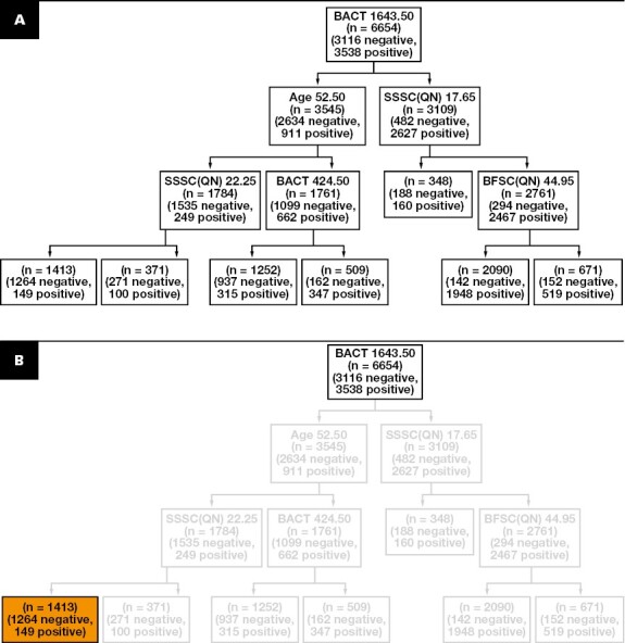
Tree-pruning strategy. A, Generation of the initial decision tree using the standard configuration of sk-learn. B, Selection of the end node by the identification of the node with the highest number of negative samples (in orange) while keeping the number of positive within the sensitivity threshold.

In addition to this analysis based on classic CART DT, we conducted additional experiments to investigate whether it was possible to improve the classification power of the DT while retaining its innate interpretability. To achieve this, we implemented a procedure that applies lookahead in the creation of the tree splits.

Decision Trees With Lookahead

The DTs apply a variety of induction algorithms that are based on traditional heuristic techniques to split the nodes and create the tree. Popular greedy algorithms like CART have proven to work well in practice but still sometimes manifest the flaws of the greedy approaches, like convergence to local optima, leading to overfit and poor generalization. To overcome this, a “lookahead” approach was implemented.

In traditional DTs, each node represents a decision point based solely on the current state of the system. Lookahead DTs, on the other hand, consider future states of the system when making decisions. The lookahead strategy works by simulating the effects of each possible decision at each node in the tree and then selecting the decision that leads to the best outcome in the long run. This allows the DT to take into account not only the immediate consequences of a decision but also the future consequences, which can result in better overall performance. Oversimplifying the concept, classic DTs select the best features one at a time, while the lookahead procedure allows it to consider different combinations of features, in order to find the best.

FIGURE 3 shows an example with a table containing a small data set, the creation of a regular tree, and a tree with a 1-step lookahead. The data set exemplifies the case where a test with a certain outcome (positive if 1, negative if 0) is performed on 8 samples where the age and the sex of the samples’ patients are given. On the basis of these data, we want to create a model that classifies the outcome of the test based on the age and sex of the patient. A quick glance at the data set reveals that the male patients are younger than the female ones and that the outcome depends on the age of the patients.

FIGURE 3.

Example of the lookahead procedure. A, The data set shows 8 samples with patients with a certain age, sex, and the outcome of the test. The classic decision tree (B) is not able to recognize that the first split should be done based on the sex of the patient, while the lookahead procedure (C) is more capable and achieves the perfect split of all the leaves. The color represents whether the samples are negative (orange), positive (blue), or no majority (gray).

The tree with lookahead is capable of detecting that the age threshold is different based on the sex of the patients, and therefore it first splits the patients by sex and then identifies the best age threshold on the 2 groups, resulting in perfectly pure leaves. This example presents a case where to reach an optimal result it is necessary to perform a step that is suboptimal. In fact, the split by sex at the root node is not effective because it results in highly impure leaves. The classic tree cannot perform such a split because it only focuses on immediate purity value, without caring about future implications, gaining a better split immediately after the root node but resulting in a worse overall performance.

In general, if the decision algorithm evaluates the possible outcomes of each available action (for a node) up to k moves in advance, then the obtained trees are called “k-step lookahead.” Due to the high computational time and complexity, the most popular are the 1-step and 2-step lookahead. In some cases, the benefit of using the lookahead mechanism could not be proven, with the traditional greedy approaches delivering better results. However, a 1-step lookahead approach is generally a good compromise between performance and cost, as it was shown when the dual information distance method outperformed popular classifiers.²⁴

Evaluation

To evaluate the model, we split the data set of samples with ground-truth values (ie, the 8317 samples that were screened for UC) using 80% data for training and 20% for evaluation. The split is done based on the date, so that we use the 20% most recent data for the evaluation and the rest for training. In this way, we simulate a prospective validation of the retrospective analysis. This results in 6654 samples used for training and 1663 samples used for evaluation.

Infrastructure

All tests were run on a computer equipped with AMD Ryzen 5800X3D with 8 cores at 3.4 GHz equipped with NVidia RTX 3080 and 16 GB of RAM.

RESULTS

Descriptive Statistics

After excluding pediatric patients (age <11 years) and few patients with missing features, the clinical cohort was composed of 10,534 patients with a median age of 64 years. Age followed a bimodal distribution, with a peak around age 30 years and a peak around age 80 years. The cohort was overall composed of 37% males and 63% females, although these percentages were not constant through ages. Age and sex distributions can be better visualized in Supplemental Figure 6 (all supplementary material is available at American Journal of Clinical Pathology online). Most were outpatients (79%) and the others inpatients (21%).

A total of 15,312 samples from 10,534 patients were included in the analysis. Of these samples, 8317 (54%) were deemed positive by the current laboratory screening with rule 1. Of these, 4485 (29.3%) were found positive at UC, 3052 (19.9%) negative, and 780 (5.1%) contaminated. These data are visualized in Supplemental Figure 5. This screening was adopted in 2018 with a minimum amount of false-negative samples (2%-3%) (internal historical data). Rule 1 was verified in the current study by culturing 500 samples deemed negative by the screening, of which 15 (3%) were found positive, confirming known results. The current method thus has a sensitivity of 97% with a workload reduction of 45.7%. Data are summarized in TABLE 2.

TABLE 2.

Demographic and Sample Results^a

Characteristic	Value
Patients	10,534 (100)
Age, median, y	64
Male	3896 (37.0)
Female	6638 (63.0)
Outpatients	8337 (79.1)
Inpatients	2197 (20.9)
Samples	15,312 (100)
Screening
Negative	6995 (45.7)
Positive	8317 (54.3)
Culture
Negative	3052 (19.9)
Positive	4485 (29.3)
Contaminated	780 (5.1)

^aValues are presented as number (%) unless otherwise indicated.

Decision Tree Analysis

In this analysis, we divide the features in 3 groups: scatter, derived, and clinical. Scatter and derived features are parameters given by the screening machine, and they are described in detail in the Methods section. Clinical features include age, sex, and inpatient/outpatient status.

First, we create 1 DT for each feature group so that we can evaluate the impact of each feature group on performance. Second, we create a DT containing all the features so that we can evaluate whether the combination of different features is beneficial or not. Last, we take the best set of features (one of the groups or the combination of groups) and create a DT with a lookahead of 1, to evaluate whether this procedure brings some benefits over classic DT.

Clinical Features

From the analysis on the clinical features alone, the samples are divided solely taking into account age and sex, while the inpatient/outpatient status was not deemed important by the algorithm. In particular, the end node identifies the best subset to be women aged between 30 and 32 years. In the training set, this results in 263 true negatives and 50 false negatives.

Scattering Features

From the scatter features analysis, 4 features were deemed relevant, which are descriptive of the size, complexity of the particle, and the degree of staining of the cell nucleus. The selected features to identify the negative samples are as follows:

1. BFSC, which is responsible for the size of the particles, in particular bacteria

2. SSSC, which determines the inner complexity of the particle

3. BFLH, degree of staining of the cell nucleus of bacteria particles

4. SFLH and SFLL, degree of staining of the cell nucleus of sediment and other particles

The end node shows that, based on the training data, the tree identifies 696 true negative and 66 false negatives.

Derived Features

From the derived features, BACT and WBC are confirmed as relevant features to detect negative samples, with the addition of epithelial cell (EC) count. In this case, the end node shows that, based on the training data, the tree identifies 695 true negatives and 61 false negatives. More details on these experiments can be found in the supplementary materials.

All Features

The best approach by far, however, is the tree created with all the available features. This tree is shown in FIGURE 4.

FIGURE 4.

Decision tree created with all the available features. The node in orange represents the end node, which is the node that identifies the samples classified as negative. All the other nodes, in blue, indicate the samples that are classified as positive and are sent to urine culture. For definitions of abbreviations, see TABLE 1.

Note that, while it could seem obvious that using more features would increase the performance of the model, it is not always the case, especially with models like DT, which rely on a greedy splitting procedure to decide the most important feature. In this case, the selected features are a combination of the best features seen on the dedicated trees: in particular, BACT and JUMUCUS from the derived features, Age from the clinical, and SSSC, BFSC, and BFLH from the scatter features. Interestingly, all these features were deemed as important already in their respective trees (being clinical, scatter, or derived). The only exception is JUMUCUS, which is a feature that was introduced in this tree and indicates the presence of mucus in the sample.

The end node shows that, based on the training data, the tree identifies 1023 true negatives and 70 false negatives. The resulting rule from the given tree is the following:

$${\displaystyle \begin{array}{l}{\displaystyle \begin{array}{lll}& {\displaystyle \mathrm{B}\mathrm{A}\mathrm{C}\mathrm{T}\le 1643.5\wedge \mathrm{B}\mathrm{F}\mathrm{S}\mathrm{C}>19\wedge \mathrm{A}\mathrm{g}\mathrm{e}\le 52.5\wedge \mathrm{B}\mathrm{F}\mathrm{L}\mathrm{H}\le 114.1\wedge }& {\displaystyle \mathrm{W}\mathrm{B}\mathrm{C}\le 57.5\wedge \mathrm{S}\mathrm{S}\mathrm{S}\mathrm{C}\le 22.1\wedge \mathrm{J}\mathrm{U}\mathrm{M}\mathrm{U}\mathrm{C}\mathrm{U}\mathrm{S}\le 205.6}\end{array}}\end{array}}$$ (2)

Given that the all-features tree was the best performer, we decided to use this feature set to create the advanced DT with lookahead of 1.

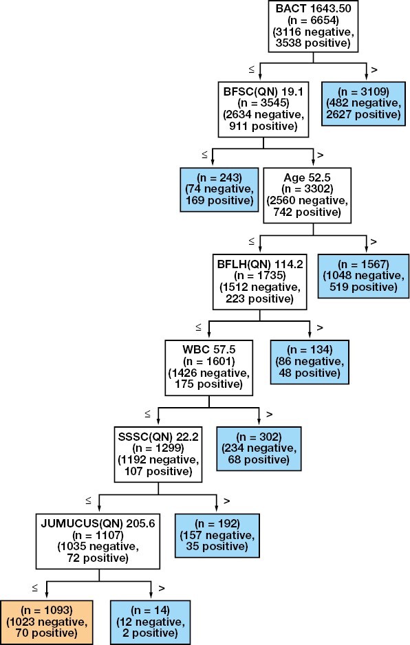
FIGURE 5 shows the tree created with all features and lookahead of 1. Based on our evaluation, this is the best-performing tree. Interestingly, the lookahead procedure confirms many features that were selected by the tree in FIGURE 4, but there are also differences that result in the lookahead tree to be simpler while achieving similar performance. In particular, starting from the root node:

FIGURE 5.

Decision tree created with all the available features and using a lookahead of 1 step to split the nodes. The tree is more compact than the counterpart without lookahead FIGURE 4 and is less prone to overfit, as shown in TABLE 3. For definitions of abbreviations, see TABLE 1.

• The age threshold is very similar in the 2 trees (52 vs 48 years).

• The BACT threshold is much higher, excluding the patients with a large number of bacteria.

• Concerning BFLH, the upper bound of 113.5 is confirmed, but it is refined with the addition of a lower bound, meaning that samples are selected if the BFLH is between 75.5 and 113.5.

• SFLL is correlated to the nucleus size and granularity content of the cell. It is not present in the all-features tree without lookahead but is actually present in the tree built with the scatter features only, with a very similar threshold.

• JUMUCUS is identified by both trees as the best feature for the final split but with different thresholds.

These differences result in a rule that is much more compact than rule 2:

$${\displaystyle \begin{array}{l}{\displaystyle \begin{array}{lll}& {\displaystyle \mathrm{A}\mathrm{g}\mathrm{e}\le 48\wedge \mathrm{B}\mathrm{A}\mathrm{C}\mathrm{T}\le 4,523.2\wedge 75.5\le \mathrm{B}\mathrm{F}\mathrm{L}\mathrm{H}\le 113.5\wedge }& {\displaystyle \mathrm{S}\mathrm{F}\mathrm{L}\mathrm{L}\le 114.9\wedge \mathrm{J}\mathrm{U}\mathrm{M}\mathrm{U}\mathrm{C}\mathrm{U}\mathrm{S}\le 67.1}\end{array}}\end{array}}$$ (3)

Given that our goal is to maximize the number of identified negative samples at the given sensitivity threshold of 98%, classic evaluation metrics like accuracy and precision are not suited to evaluate the performance of the trees. In particular, we are interested in maximizing the workload reduction, without exceeding the sensitivity threshold. TABLE 3 summarizes the results of the 5 trees on the training and evaluation set. The trees constructed with all the available features (all and all-LA-1) are by far the best performers. Note that while the tree with lookahead shows a smaller workload reduction on the training set, it actually shows better reduction on the evaluation set, at the expense of less false negatives. In other words, the lookahead model is less prone to overfit, probably because it is a more “parsimonious”model. Overfitting occurs when a model learns not only the underlying patterns in the training data but also the noise or random fluctuations. Consequently, an overfitted model performs well on the training data but poorly on unseen data (test data) because it essentially fails to generalize. Such a model might make unreliable or overly confident predictions when exposed to new data. One approach to mitigate overfitting is through the use of “parsimonious” models, which accomplish the desired level of explanation or prediction with as few predictors as necessary. In essence, a parsimonious model is a simpler model with fewer parameters. Parsimonious models generally reduce the overfitting potential and are more robust to noise, more interpretable, and less resource demanding. The larger degree of parsimony of the lookahead tree can be easily seen from its logic rule, which is more compact and simple than the other one (see comparison between rule 2 and rule 3). Thus, we select the lookahead tree FIGURE 5 as the best model for our evaluation and rule 3 as the rule that needs to be applied in combination with the preexisting rule 1 as follows:

TABLE 3.

Summary of the Results of All the Trees Created on the Different Feature Sets^a

	Training set, %		Evaluation set, %
Feature set	False negative	Reduction	False negative	Reduction
Clinical	1.41	3.95	1.37	3.13
Scatter	1.87	10.46	2.75	11.91
Derived	1.72	10.44	2.32	11.06
All	1.98	15.37	2.85	15.87
All L-A 1	1.95	13.99	2.64	16.00

^aThe table shows the percentage of false negatives and achieved workload reduction for the training set and the evaluation set, respectively.

$${\displaystyle \begin{array}{l}{\displaystyle \begin{array}{llll}& {\displaystyle \left(\mathrm{r}\mathrm{u}\mathrm{l}\mathrm{e}1\right)\vee \left(\mathrm{r}\mathrm{u}\mathrm{l}\mathrm{e}3\right)=(\mathrm{B}\mathrm{A}\mathrm{C}\mathrm{T}\le 100\wedge \mathrm{W}\mathrm{B}\mathrm{C}\le 75\wedge \mathrm{Y}\mathrm{S}\mathrm{T}\le 30)\vee }& {\displaystyle (\mathrm{A}\mathrm{g}\mathrm{e}\le 48\wedge \mathrm{B}\mathrm{A}\mathrm{C}\mathrm{T}\le 4523.2\wedge 75.5\le \mathrm{B}\mathrm{F}\mathrm{L}\mathrm{H}}& {\displaystyle \le 113.5\wedge \mathrm{S}\mathrm{F}\mathrm{L}\mathrm{L}\le 114.9\wedge \mathrm{J}\mathrm{U}\mathrm{M}\mathrm{U}\mathrm{C}\mathrm{U}\mathrm{S}\le 67.1)}\end{array}}\end{array}}$$ (4)

In addition to the described analysis, we made an attempt at realizing 2 different models for male/female and inpatient/outpatient status. The models actually performed worse than the undifferentiated DT. This is in accordance with the fact that the DT never showed sex or inpatient/outpatient status as relevant split nodes. By creating 2 different DTs for these categories, it is like enforcing a (suboptimal) splitting criterion at the root of the tree. Furthermore, poor performance could be due to the strong imbalance of the data set in favor of female outpatients, leading to poor-performing trees with a relatively smaller data set of male/inpatients. Results are reported in supplementary data.

DISCUSSION

Besides a few studies enrolling fewer than 1000 patients, the only studies that have employed ML tools to predict the result of UC are Burton et al¹⁵ and Taylor et al.²⁵ The study by Taylor et al,²⁵ though, aims at predicting UTI in general, in the setting of an emergency department, with availability of a large number of clinical features, medical history, signs, and symptoms. These data are not typically available in a microbiology laboratory and cannot be easily implemented to optimize the laboratory workflow. The work by Burton et al¹⁵ is more similar to our study, with the same aim of optimizing the urine screening by automated analyzers. The study explored a heuristic model (WBC and bacteria) and other supervised ML models (neural networks, random forest, XGBoost, etc) in a cohort much larger than ours (220,000 samples). Despite excellent results, proposed models cannot be easily implemented inside an automated analyzer. The software of UF-1000i, for example, allows for the implementation of simple logic rules and cannot be programmed to classify samples based on more complex ML models. As a matter of fact, Burton et al¹⁵ implemented only the heuristic model in the clinical routine, which overlaps with the already widespread rule of WBC and bacteria. The ML models remained on paper since they did not enter the clinical routine. Besides the technical difficulties of implementing such models into automated analyzers, which could be overcome sooner or later, the fact that many ML models are not interpretable is an additional obstacle to real-world implementation. A medical environment needs transparent rules that can be trusted and validated periodically. For this reason, the importance of a fully interpretable model in medicine cannot be underestimated for multiple reasons: in the best of cases, an interpretable model can be translated in a set of logic rules, and these can be easily implemented in current laboratory devices, but most important, the medical professional is not forced to blindly rely on the model but is able to look at the reasoning behind classification, and this generates trust; furthermore, there is still no clear consensus on how to deal with nontransparent classification models from an ethical and legal perspective.

In this context, it is important to acknowledge that advancements have been made in enhancing the explainability of traditional “black box” models, such as neural networks. For instance, the LIME (Local Interpretable Model-agnostic Explanations)²⁶ method provides explanations for individual predictions made by complex models by approximating them with interpretable models that are locally faithful. Another approach is SHAP (SHapley Additive exPlanations),^27,28 which is based on cooperative game theory and assigns each feature an importance value for a particular prediction. These methods, together with quantification of uncertainties of ­prediction,²⁹ are contributing to bridging the gap between accuracy and interpretability, making neural networks more transparent and, as a result, more accessible for use in sensitive domains such as health care. Nevertheless, it is essential to highlight the distinct transparency and linearity of rules within DTs. In DTs, the model is formulated as a clear and linear sequence of logic rules based on feature values, making them naturally interpretable. Conversely, in more complex models such as neural networks, the utilization of features can be intricate and even obscure. Although methods like LIME and SHAP can provide some level of explainability, the inherent nonlinearity and complexity of these models mean that their feature utilization is rarely as transparent or easily interpretable as in DTs. In addition, in our specific scenario, practical constraints necessitated the implementation of a logic rule directly on the device. This was due to the absence of available middleware solutions that would allow for the deployment of complex ML models. The integration of sophisticated models into the device would necessitate an intermediary layer for interpretation and implementation, which was not feasible in our case.

This gives us the opportunity to discuss that laboratory medicine might need to begin to consider environments enabled by middleware or other architectures that will allow for ML models to be more routinely brought into clinical use. This could bring several benefits to the field: first and foremost, it allows for the utilization of advanced models to enhance diagnostic accuracy. Furthermore, such middleware would facilitate data-driven research and quality improvement initiatives in laboratory medicine. By leveraging large-scale data collected within laboratory systems and from multiple devices, researchers can develop, validate, and monitor novel ML algorithms; identify new biomarkers; and uncover hidden patterns in complex data sets. This would require a multidisciplinary effort but could unlock the full potential of data science in laboratory medicine.

In our laboratory, the current screening approach identifies a sample as negative when it has both white blood cells less than 75 and bacteria less than 100. This excludes 6995 (45.6%) samples, leaving 8317 samples to be cultured. Starting from these samples, the DT presented in this study identifies an additional 16% of samples (1330 annually) that could be safely excluded from cultures, at the cost of 2.6% false negatives (217 annually). This brings the current effectiveness of the screening in workload reduction from 45.6% to 54.5% of the total, at the cost of 5.5% sensitivity.

In our case, with around 15,000 samples per year, the impact of the presented results on the financial balance of the laboratory would be around 40,000 euros/y, based on an estimated culture cost of 30 euros³⁰ multiplied by approximately 1400 samples screened out by the new set of rules. For smaller or bigger laboratories, results would scale accordingly.

The negative samples are identified by rule 3 having bacteria <4523, years <48, 75 < BFLH < 114, SFLL <114, and JUMUCUS <67 in addition to the precondition of rule 1.

The first 2 features, bacteria and age, can be easily interpreted and match everyday clinical experience: younger patients with a relatively lower bacterial count are less prone to have a real infection ongoing. Four thousand bacteria roughly corresponds to the 80th percentile, meaning that the algorithm excludes the 20% of the highest bacterial count, which are more likely to have a real infection.

The meaning of the age cutoff can be visualized by plotting the distribution of positive and negative samples against the age (Supplemental Figure 6). The age of 48 years corresponds to the point over which there is an inversion in the distribution of positive and negative samples. Below the age cutoff, negative samples are more prevalent, while over the age cutoff, positive samples become more prevalent. As a logical consequence, with the aim of avoiding unnecessary cultures, it is more convenient to focus on the area where negative samples are prevalent, which is age younger than 48 years.

While the first parameters (bacteria and age) are self-explanatory, scattering values SFLL and BFLH need some explanation. The Sysmex UF-1000i works by taking 2 aliquots of the urine sample and processing them separately. One is used to study the sediment (S) and the other to study bacteria (B). The aliquots are stained with polymethine dyes, and the signal of fluorescent light (FL) is subject to 2 different types of amplification, named high (H) and low (L), which corresponds to 2 different scattergrams used to discriminate clusters/type of cells. SFLL thus refers to the sediment aliquot (S), fluorescence light (FL), amplified at low level (L); BFLH refers to the bacteria aliquot (B), fluorescence light (FL), amplified at high level (H). SFLL is correlated to the nucleus size and granularity content of the cell. BFLH represents the degree of staining of the cell nucleus of bacteria particles.

The cutoff shown by the algorithm to identify a more relevant fraction of negative samples is SFLL <114 and BFLH <114. For SFLL, the cutoff corresponds grossly to the first quartile value of SFLL (30th percentile).

The clustering of different cell types with respect to SFLL is represented in FIGURE 1. Lower values are where the WBC cluster starts to merge with the YLC and bacteria clusters, increasing the risk of misclassification. This suggests that SFLL <114 points toward samples with higher chances of WBC misclassification and thus samples with potential overestimation of WBC. WBCs are the mainstay of UTI, so if WBCs are overestimated, then the sample is falsely deemed positive when it should have been deemed negative. This supports the opinion that including raw data in ML models adds useful information.

About BFLH, the cutoffs of 75 and 114 identify an interval roughly between the 10th and the 85th percentiles. BFLH represents the degree of staining of the cell nucleus of bacteria particles. Looking at the scattergram in Supplemental Figure 7, it is possible to verify that high values of BFLH are associated with bacteria. In particular, the tree ensures that samples lying on the highest 15th percentile of BFLH, and therefore associated with an elevated presence of bacteria, are classified as positive and sent to culture. At the same time, it excludes samples lower than the 10th, which are typically associated with debris.

BFSC correlates with the size of the microorganism. At first, we were puzzled by this evidence because this would mean that larger bacteria (Gram negative) are more often associated with negative samples than smaller bacteria (Gram positive). Clinically, we actually expected the opposite, because Gram positive might be present in harmless colonization of skin bacteria, while Gram negative is almost always associated with an active infection. We found the answer in the literature, where De Rosa et al⁴ demonstrated that a value of BFSC below 30 strongly indicates the presence of Gram negative. Their interpretation, with which we agree, is that the larger forward scatter of Gram positive is most likely due to their conformation in chains (streptococci) and clusters (staphylococci).

It is important to acknowledge that the identified cutoffs are not to be considered exact and immutable but could reflect peculiarities of our data set and may slightly vary based on different data sets. However, it is not the exact value of the cutoff that is important but rather that the population is split in a way that complies with existing knowledge. The aforementioned observations provide valuable insights into the biology of urine screening, which can be substantiated through clinical reasoning and experience. This, in turn, contributes to the algorithm transparency, ultimately enhancing its overall integrity.

The study has 1 major limitation: the total amount of data collected (~15,000 samples) is subject to a preexisting screening rule (rule 1), where about 45% of the samples are screened as negative and are not sent to culture. This means that for those samples, we do not have the ground truth of the bacterial growth. Rule 1 was validated in the course of the current study by culturing 500 samples deemed negative by the screening, of which 15 (3%) were found positive, confirming known results. Thus, in our analysis, we could only evaluate the subset of 8317 samples that were sent to culture, taking into account that there was an estimated 3% false negatives overall. Due to this, we had to set a very high threshold of sensitivity on our algorithm (98%), in order to set a minimum sensitivity of 95% on the training set for the combination of the existing screening rule and our new algorithm. This sensitivity constraint resulted in a sensitivity of 94.5% in the validation set, achieving a 16% workload reduction. For this reason, we believe that the implementation of our algorithm on a whole unscreened data set has the potential of delivering better results.

Another limitation of the study is that patient entries do not have clinical data or labels such as preexisting conditions, previous UTI, or comorbidities. The integrated evaluation of such features might lead to better results.

The study is based on data collected from an obsolete system (Sysmex UF-1000i) that has been replaced by a new version (Sysmex UF-5000) with added features such as discrimination between Gram positive and Gram negative,³¹ as well as renal tubular cells that proved to be useful in discriminating upper vs lower urinary tract infections.³² However, we used the data set of the UF-1000i because the newer UF-5000 does not offer the possibility to extract raw scattering values, which in our hypothesis were possibly more informative than partially processed data for generating a ML model. Mainly for this reason, the model cannot be simply implemented on the better-equipped UF-5000. As a lesson learned from this point, in our opinion, companies should always allow release of raw data as output of devices.

Another limitation of this study, which might be overcome by additional work, is the lack of “external” validation (ie, validation on an data set collected by another laboratory). The preanalytical phase highly affects modern urinalysis³³: as preanalytical conditions are highly variable from center to center, results show a marked interlaboratory variability. For this reason, the degree of generalizability and the variation of the model performance between different laboratories are unknown and require further investigation.

The absence of a label marking the sample as collected from urine catheterization is also a limitation. Catheterization, in fact, could cause artifacts in cellular elements, leading to an altered set of values. Such samples might be treated more effectively by the algorithm if labeled.

CONCLUSION

We demonstrated a DT model that can reduce the workload of a microbiology laboratory by an additional 16% of the remaining samples after the initial reduction of 45% when rule 1 is applied while maintaining a sensitivity level of 94.5%. This means that the cutoffs identified by the tree build on top of the existing rule, and therefore all samples that were classified negative by rule 1 are still classified as negative in our model. Our model was created using decision trees as a base and then applying an ad hoc pruning strategy. In addition, we also implemented a lookahead procedure that increases the training time but helps to control the overfit of the model, improving the performance. The model is completely interpretable and based on bacteria count and mucus count per microliter, age, and 2 scattering parameters. Our results show that the raw scatter parameter of the machine is of nonnegligible importance. The criteria employed by the model are supported by literature. The model can be readily implemented in the Sysmex UF-1000 without the need of additional software or technological improvement. In particular, rule 4 shows the formula to be used in order to identify negative samples, improving the existing rule. Further validation with an external data set is suggested before considering the model in general.

Conflict of interest disclosure: The authors have nothing to disclose.

REFERENCES

- 1. Boonen K, Koldewijn E, Arents N, Raaymakers P, Scharnhorst V.. Urine flow cytometry as a primary screening method to exclude urinary tract infections. World J Urol. 2013;31(3):547-551. [DOI] [PubMed] [Google Scholar]
- 2. Broeren M, Bahçeci S, Vader H, Arents N.. Screening for urinary tract infection with the Sysmex UF-1000i urine flow cytometer. J Clin Microbiol. 2011;49(3):1025-1029. [DOI] [PMC free article] [PubMed] [Google Scholar]
- 3. Enko D, Stelzer I, Böckl M, et al. Comparison of the reliability of Gram-negative and Gram-positive flags of the Sysmex UF-5000 with manual Gram stain and urine culture results. Clin Chem Lab Med. 2021;59(3):619-624. [DOI] [PubMed] [Google Scholar]
- 4. De Rosa R, Grosso S, Bruschetta G, et al. Evaluation of the Sysmex UF1000i flow cytometer for ruling out bacterial urinary tract infection. Clin Chim Acta. 2010;411(15-16):1137-1142. [DOI] [PubMed] [Google Scholar]
- 5. De Rosa R, Grosso S, Lorenzi G, Bruschetta G, Camporese A.. Evaluation of the new Sysmex UF-5000 fluorescence flow cytometry analyser for ruling out bacterial urinary tract infection and for prediction of Gram negative bacteria in urine cultures. Clin Chim Acta. 2018;484:171-178. 10.1016/j.cca.2018.05.047 [DOI] [PubMed] [Google Scholar]
- 6. Jimenez-Guerra G, Heras-Cañas V, Valera-Arcas M, Rodrıguez-Granger J, Navarro J, Gutierrez-Fernandez J.. Comparison between urine culture profile and morphology classification using fluorescence parameters of the Sysmex UF-1000i urine flow cytometer. J Appl Microbiol. 2017;122(2):473-480. [DOI] [PubMed] [Google Scholar]
- 7. Grosso S, Bruschetta G, De RR, Avolio M, Camporese A.. Improving the efficiency and efficacy of pre-analytical and analytical work-flow of urine cultures with urinary flow cytometry. New Microbiol. 2008;31(4):501-505. [PubMed] [Google Scholar]
- 8. García-Coca M, Gadea I, Esteban J.. Relationship between conventional culture and flow cytometry for the diagnosis of urinary tract infection. J Microbiol Methods. 2017;137:14-18. [DOI] [PubMed] [Google Scholar]
- 9. Pieretti B, Brunati P, Pini B, et al. Diagnosis of bacteriuria and leukocyturia by automated flow cytometry compared with urine culture. J Clin Microbiol. 2010;48(11):3990-3996. 10.1128/JCM.00975-10 [DOI] [PMC free article] [PubMed] [Google Scholar]
- 10. Sun S, Zuo L, Liu P, Wang X, He M, Wu S.. The diagnostic performance of urine flow Cytometer UF1000i for urinary tract infections. Clin Lab. 2018;64(9):1395-1401. [DOI] [PubMed] [Google Scholar]
- 11. Íñigo M, Coello A, Fernández-Rivas G, et al. Evaluation of the SediMax automated microscopy sediment analyzer and the Sysmex UF-1000i flow cytometer as screening tools to rule out negative urinary tract infections. Clin Chim Acta. 2016;456:31-35. [DOI] [PubMed] [Google Scholar]
- 12. Jolkkonen S, Paattiniemi E, Karpanoja P, Sarkkinen H.. Screening of urine samples by flow cytometry reduces the need for culture. J Clin Microbiol. 2010;48(9):3117-3121. [DOI] [PMC free article] [PubMed] [Google Scholar]
- 13. Manoni F, Fornasiero L, Ercolin M, et al. Cutoff values for bacteria and leukocytes for urine flow cytometer Sysmex UF-1000i in urinary tract infections. Diagn Microbiol Infect Dis. 2009;65(2):103-107. 10.1016/j.diagmicrobio.2009.06.003 [DOI] [PubMed] [Google Scholar]
- 14. Monsen T, Ryden P.. A new concept and a comprehensive evaluation of SYSMEX UF-1000i flow cytometer to identify culture-negative urine specimens in patients with UTI. Eur J Clin Microbiol Infect Dis. 2017;36(9):1691-1703. 10.1007/s10096-017-2964-1 [DOI] [PMC free article] [PubMed] [Google Scholar]
- 15. Burton R, Albur M, Eberl M, Cuff S.. Using artificial intelligence to reduce diagnostic workload without compromising detection of urinary tract infections. BMC Med Inform Decis Mak. 2019;19(1):171. [DOI] [PMC free article] [PubMed] [Google Scholar]
- 16. Roux-Dalvai F, Gotti C, Leclercq M, et al. TNA. Fast and accurate bacterial species identification in urine specimens using LC-MS/MS mass spectrometry and machine learning. Mol Cell Proteomics. 2019;18(12):2492-2505. [DOI] [PMC free article] [PubMed] [Google Scholar]
- 17. Lee KS, Lim HJ, Kim K, Park YG, Yoo JW, Yong D.. Rapid bacterial detection in urine using laser scattering and deep learning analysis. Microbiol Spectr. 2022;10(2):e0176921. [DOI] [PMC free article] [PubMed] [Google Scholar]
- 18. Podgorelec V, Kokol P, Stiglic B, Rozman I.. Decision trees: an overview and their use in medicine. J Med Syst. 2002;26(5):445-463. 10.1023/a:1016409317640 [DOI] [PubMed] [Google Scholar]
- 19. Quinlan JR. Induction of decision trees. Mach Learn. 1986;1(1):81-106. 10.1007/bf00116251 [DOI] [Google Scholar]
- 20. Quinlan JR. Simplifying decision trees. Int J Man-Mach Stud. 1987;27(3):221-234. 10.1016/s0020-7373(87)80053-6 [DOI] [Google Scholar]
- 21. Quinlan JR. C4.5: Programs for Machine Learning. Elsevier; 1992. [Google Scholar]
- 22. Breiman L, Friedman J.. CJSRAO. In: Classification and Regression Trees. Routledge; 1984. [Google Scholar]
- 23. Hancock T, Jiang T, Li M, Tromp J.. Lower bounds on learning decision lists and trees. In: STACS 95. Springer; 1995:527-538. [Google Scholar]
- 24. Ben-Gal I, Dana A, Shkolnik N, Singer G.. Efficient construction of decision trees by the dual information distance method. Qual Technol Quant Manag. 2014;11(1):133-147. 10.1080/16843703.2014.11673330 [DOI] [Google Scholar]
- 25. Taylor RA, Moore CL, Cheung KH, Brandt C.. Predicting urinary tract infections in the emergency department with machine learning. PLoS One. 2018;13(3):e0194085. 10.1371/journal.pone.0194085 [DOI] [PMC free article] [PubMed] [Google Scholar]
- 26. Ribeiro MT, Singh S, Guestrin C. “Why should I trust you?”: explaining the predictions of any classifier. arXiv. 2016. [Google Scholar]
- 27. Shapley LS.. A value for n-person games. In: Kuhn HW, Tucker AW, eds. Contributions to the Theory of Games II. Princeton University Press; 1953:307-317. [Google Scholar]
- 28. Lundberg SM, Lee SI.. A unified approach to interpreting model predictions. In: Guyon I, Luxburg UV, Bengio S, et al, eds. Advances in Neural Information Processing Systems. Curran Associates; 2017;30:4765-4774. [Google Scholar]
- 29. Abdar M, Pourpanah F, Hussain S, et al. A review of uncertainty quantification in deep learning: techniques, applications and challenges. Inf Fusion. 2021;76:243-297. 10.1016/j.inffus.2021.05.008 [DOI] [Google Scholar]
- 30. Xu R, Deebel N, Casals R, Dutta R, Mirzazadeh M.. A new gold rush: a review of current and developing diagnostic tools for urinary tract infections. Diagnostics. 2021;11(3):479. 10.3390/diagnostics11030479 [DOI] [PMC free article] [PubMed] [Google Scholar]
- 31. Yang SSD, Yang CC, Chen YS, Chang SJ.. A performance comparison of the fully automated urine particle analyzer UF-5000 with UF-1000i and Gram staining in predicting bacterial growth patterns in women with uncomplicated urinary tract infections. BMC Urol. 2021;21(1):1-6. [DOI] [PMC free article] [PubMed] [Google Scholar]
- 32. Oyaert M, Speeckaert M, Boelens J, Delanghe JR.. Renal tubular epithelial cells add value in the diagnosis of upper urinary tract pathology. Clin Chem Lab Med. 2020;58(4):597-604. [DOI] [PubMed] [Google Scholar]
- 33. Delanghe JR, Speeckaert MM.. Preanalytics in urinalysis. Clin Biochem. 2016;49(18):1346-1350. 10.1016/j.clinbiochem.2016.10.016 [DOI] [PubMed] [Google Scholar]
Associated Data
This section collects any data citations, data availability statements, or supplementary materials included in this article.