Phantom oscillations in principal component analysis

Significance

Dimensionality reduction simplifies high-dimensional data into a small number of representative patterns. One dimensionality reduction method, principal component analysis (PCA), often selects oscillatory or U-shaped patterns, even when such patterns do not exist in the data. These oscillatory patterns are a mathematical consequence of the way PCA is computed rather than a unique property of the data. We show how two common properties of high-dimensional data can be misinterpreted when visualized in a small number of dimensions.

Abstract

Principal component analysis (PCA) is a dimensionality reduction method that is known for being simple and easy to interpret. Principal components are often interpreted as low-dimensional patterns in high-dimensional space. However, this simple interpretation fails for timeseries, spatial maps, and other continuous data. In these cases, nonoscillatory data may have oscillatory principal components. Here, we show that two common properties of data cause oscillatory principal components: smoothness and shifts in time or space. These two properties implicate almost all neuroscience data. We show how the oscillations produced by PCA, which we call “phantom oscillations,” impact data analysis. We also show that traditional cross-validation does not detect phantom oscillations, so we suggest procedures that do. Our findings are supported by a collection of mathematical proofs. Collectively, our work demonstrates that patterns which emerge from high-dimensional data analysis may not faithfully represent the underlying data.

In the age of big data, high-dimensional statistics have risen from a novelty to a necessity. Dimensionality reduction methods aim to summarize high-dimensional data in just a few dimensions and expose simple low-dimensional patterns embedded within high-dimensional space. One of the simplest dimensionality reduction methods is principal component analysis (PCA) (1, 2). PCA is useful because it can be computed quickly using a compact matrix equation and can be understood without extensive mathematical training. It has gained popularity in neuroscience because the output can be interpreted as low-dimensional patterns embedded within high-dimensional data, such as trajectories through time, or spatial patterns. Interpreting PCA in this way has led to numerous neuroscientific discoveries about diverse phenomena (3–12).

While many types of low-dimensional patterns are common in neuroscience, one of the most salient patterns is oscillations. Oscillations in the brain have been studied for over a century (13). They occur in both time and space and play a crucial role in diverse functions such as memory, sleep, and development (14–17). While oscillations are important to understanding brain function, prior work has warned about a complicated relationship between oscillations and PCA (18–22). Strikingly, these studies reported examples of nonoscillatory data that had oscillatory principal components. If this phenomenon is widespread across a variety of data, it could substantially change the interpretation of PCA. In order to trust the results of PCA, it is urgent to understand what causes these oscillations.

Here, we show how and why PCA yields oscillations when no oscillations are present in the data. These “phantom oscillations” are a statistical phenomenon that explains a large fraction of variance despite having little to no relationship with the underlying data. We find two distinct properties of data which cause phantom oscillations through different mechanisms: smoothness and shifts in time or space. For each, we provide mathematical proofs and examples demonstrating their impact on data analysis. Finally, we show why traditional cross-validation is ineffective at controlling for phantom oscillations and propose alternative methods to do so. Collectively, this work illustrates how high-dimensional data analysis is intrinsically linked to low-level properties of the data.

Results

Phantom Oscillations in PCA.

Principal component analysis produces a low-dimensional representation of a high-dimensional dataset (Fig. 1A). It takes as its input a set of observations, each consisting of several features, in the form of a matrix. For example, an observation may be a neuron or brain region, a subject, or a trial, and each feature may be the point in time at which that measurement was made. Each “principal component” (PC) consists of a) a vector of “loadings” or an “eigenvector,” which correspond to patterns in the features; b) a vector of “scores,” or “weights,” corresponding to patterns in the observations; and c) the variance explained by the cross product of these two patterns, also known as the “eigenvalue.” PCA is computed by finding the eigenvectors and eigenvalues of the covariance matrix of the data (Fig. 1B). The scores are computed by multiplying the data matrix by the loadings, equivalent to a projection of the data onto the eigenvectors (Fig. 1C). In what follows, unless otherwise specified, we will focus on datasets of timeseries, where each observation is a neural signal, and each feature is a point in time. In SI Appendix, we also consider the opposite case of the transposed data matrix, meaning each observation is a point in time and each feature is a neural signal.

Fig. 1.

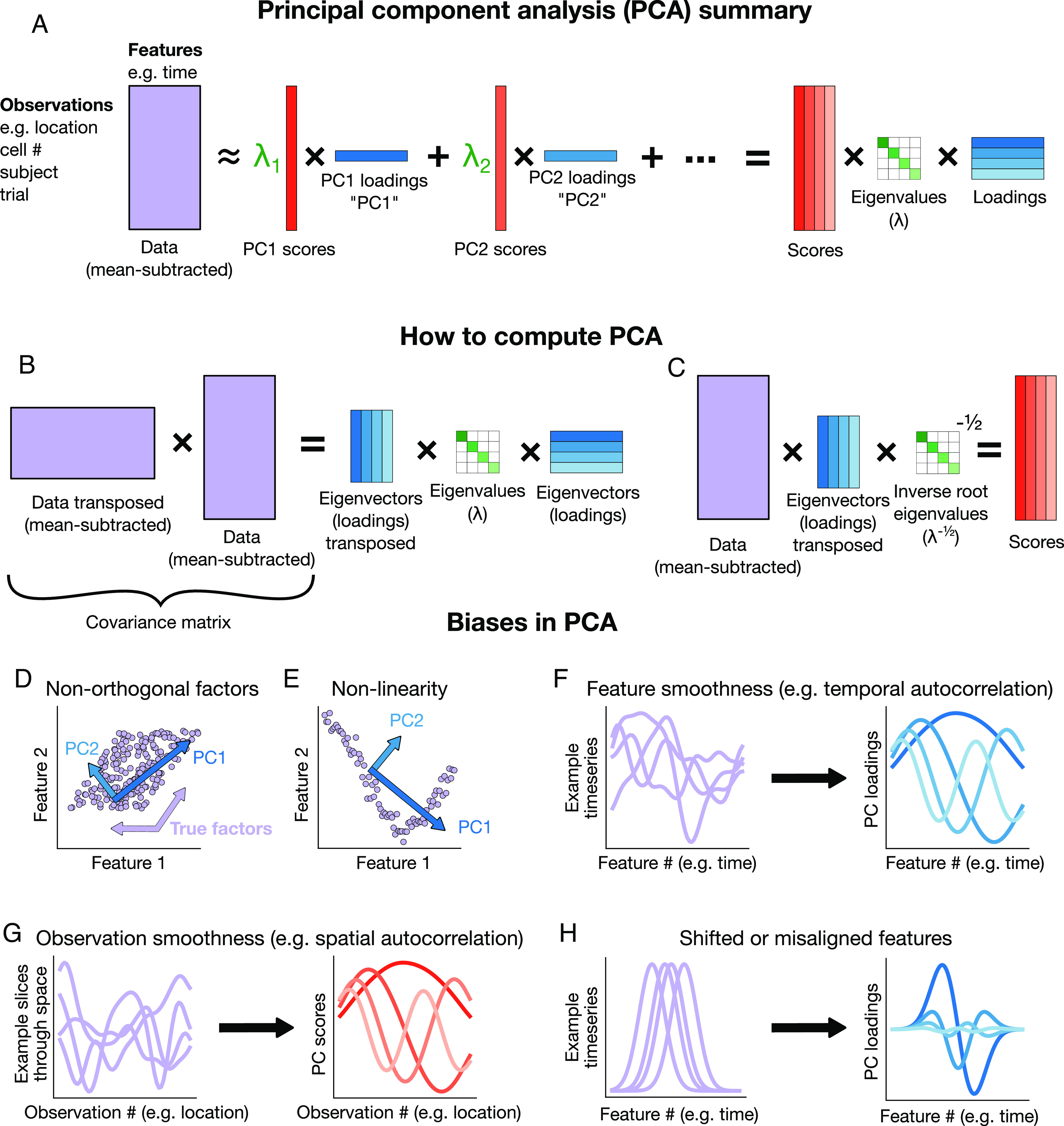
Summary of biases in PCA (A) Schematic including terminology we use throughout. (B) Summary of how to compute principal components (PCs). (C) Summary of how to compute scores. (D–H) Illustrations of (D) nonorthogonality bias, (E) nonlinearity bias, (F) smooth features leading to oscillatory loadings, (G) smooth observations leading to oscillatory scores, and (H) time-shifted features leading to oscillatory loadings.

While PCA itself does not make assumptions about the data, the most popular interpretation of PCA does. This classic interpretation posits that patterns in the loadings or scores indicate some latent underlying patterns in the data. This interpretation relies on four assumptions and may be misleading if those assumptions are violated. First, the underlying patterns must exist and be independent of one another. Second, they must combine linearly to form the observed data. Third, the data must contain exclusively these patterns and additive, uncorrelated noise. Fourth, observations must be independent. When any of these does not hold, the above interpretation of PCA may not hold.

What happens if these assumptions are violated? Violations of the first and second assumptions—independence and linearity of patterns—are known to impact data analysis (23) and are discussed at length in statistics textbooks (24). Namely, when the latent underlying patterns are not independent of each other, PCA will output components which fail to capture any of the correlated factors (Fig. 1D), and if the underlying components are not linear, then PCA will find the best linear approximation (Fig. 1E). However, less effort has gone into understanding violations of the final two assumptions: exclusivity and independence of observations (25).

The third and fourth assumptions are critical to understand because they are violated by most neuroscience data. There are multiple ways these assumptions may be violated. For example, both assumptions are violated by smoothness. Data are smooth across time, or temporally autocorrelated, if nearby points in time have similar values (Fig. 1 F, Left). Smoothness across time is a pattern which cannot be easily expressed as an additive sum, violating the third assumption. As a result, when PCA is performed on smooth timeseries, it will not exhibit interpretable components, because no single pattern can express smoothness across time. Instead, components will exhibit oscillations in the loadings (Fig. 1 F, Right) (mathematical explanation and proofs in SI Appendix). Likewise, smoothness across space, or spatial autocorrelation, occurs when observations are made at spatial locations, and nearby locations are more similar to each other than distant locations. If nearby locations are similar to each other, they will be correlated, which violates the fourth assumption that observations are independent. Smoothness across space produces oscillations in the scores (Fig. 1G).

Another common example in neuroscience which violates both the third and fourth assumptions is when observations are similar to each other but shifted in time or space (Fig. 1 H, Left). In other words, there is some underlying pattern in the data; however, this pattern occurs at a slightly different time or position in different observations. This might occur if the timing of some event can vary slightly, or if alignment is imprecise, such as a video with a shaky camera. When this occurs in time, a linear combination of features cannot succinctly represent the pattern, which violates the third assumption. When this occurs in space, then the observations are no longer independent, which violates the fourth assumption. These types of nonindependence will result in loadings that resemble temporally or spatially localized sinusoids or wavelets (Fig. 1 H, Right) (mathematical explanation and proof in SI Appendix). Smoothness and shifts are ubiquitous across timeseries and imaging data, and both lead to oscillations in PCA.

We define “phantom oscillations” as oscillations in the PCs of data that vary along a continuum. In most cases, the continuum will be time or space. In one dimension, such as timeseries, phantom oscillations resemble sine waves or localized wavelets. When plotted against each other, they often take on a characteristic “U” shape. In multiple dimensions, they resemble modes of vibration like a stationary or propagating wave, dependent on the spatial geometry of how they are sampled. Phantom oscillations may also occur on any continuum, such as a graph or a manifold in high-dimensional space. In what follows, we explore two distinct sources of phantom oscillations—smoothness and shifts—and show how they confound neuroscience data analysis.

Phantom Oscillations Caused by Smoothness in Time or Space.

Phantom oscillations arise naturally in smooth data. Almost all timeseries exhibit some amount of smoothness, so in the absence of true underlying patterns, PCA will yield oscillations. This effect can be observed on both simulated and real data. When we generated synthetic smooth timeseries using low-pass filtered white noise (Fig. 2 A, Top) and then performed PCA, we observed that the loadings resembled sinusoids (Fig. 2A, Top). The PCs for these smooth timeseries explain much more variance than the PCs for independent unsmoothed white noise timeseries, a common null model for determining the significance of PCs (Fig. 2C, Top, solid lines). The same results held when different methods were used to generate random smooth timeseries (SI Appendix, Fig. S1) and when the timeseries matrix was transposed before performing PCA (SI Appendix, Fig. S2). In each of these cases, the first and second PC approximately formed a “U” shape when plotted against each other (SI Appendix, Fig. S3). We repeated this analysis on resting state fMRI data from the Cambridge Centre for Ageing and Neuroscience (Cam-CAN) (26). To ensure no temporal structure was present across observations, we selected random segments from random brain regions and random subjects, each 118 s long (Fig. 2 A, Bottom). We again observed sinusoidal principal components (Fig. 2 B, Bottom) which explained more variance than independent white noise timeseries (Fig. 2 C, Bottom).

Fig. 2.

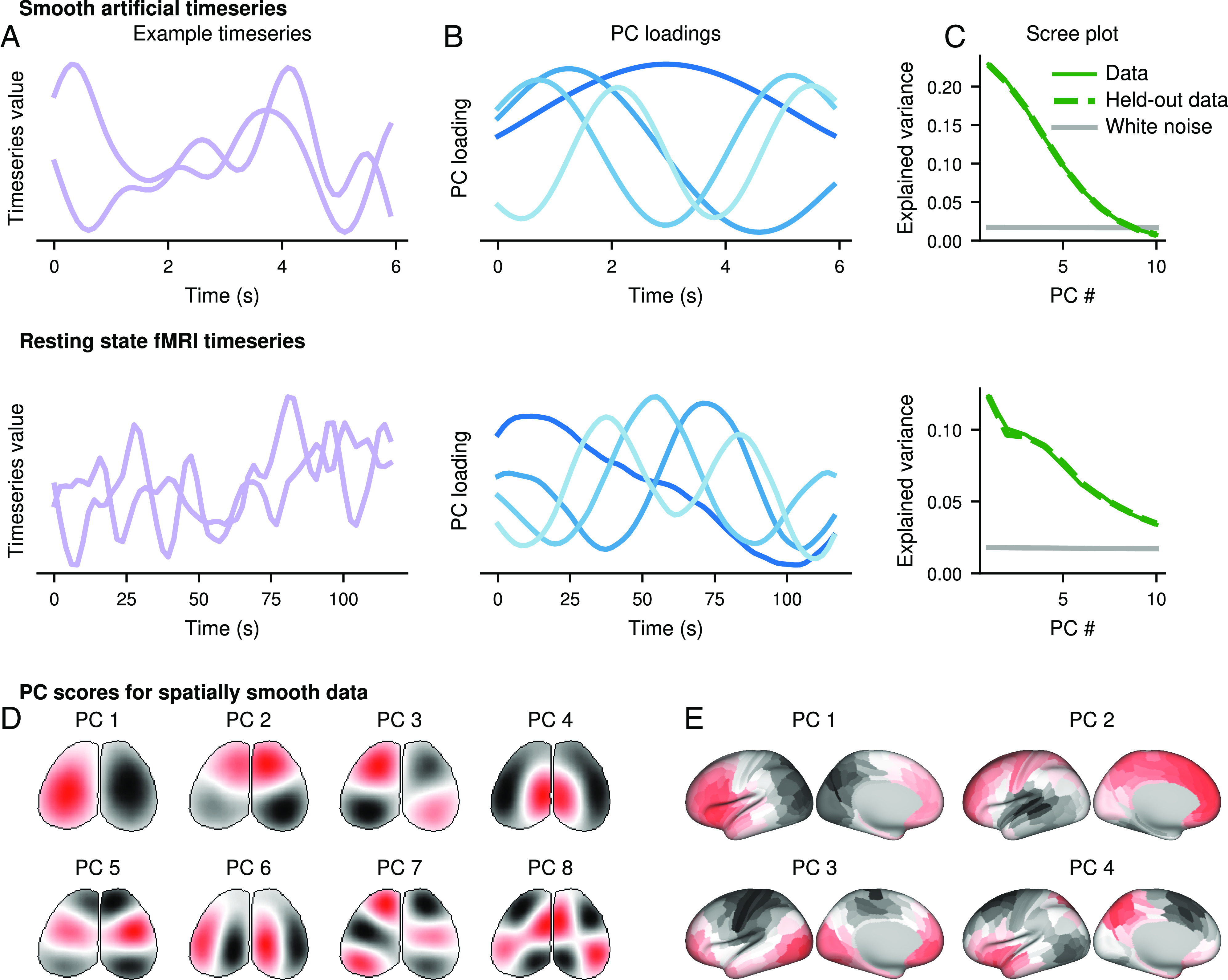
Smoothness causes phantom oscillations in PCA (A) Example timeseries for smooth artificially generated data (Top) and randomly selected segments from a resting-state fMRI scan (Bottom). (B) Loadings of the first four PCs from large populations of the artificial (Top) or fMRI (Bottom) data. (C) Variance explained by the first 10 PCs for the artificial (Top) or fMRI (Bottom) data. Solid green indicates the data from (A) and (B), and dashed green indicates a second independent sample of the same size from the same data. Gray indicates the variance explained by the first 10 PCs of an equally sized dataset of independent white noise. (D and E) Artificially generated white noise was smoothed across the spatial, but not temporal, dimension in the geometry of a widefield image (D) or a parcellated cortical surface (E). PC scores are plotted on these geometries.

These effects are not the result of overfitting and do not disappear after traditional cross-validation. To test whether cross-validation could ameliorate this effect, we generated a new independent synthetic dataset of equal size and sampled new random sequences of the Cam-CAN data. Then, we projected the new data onto the principal components from the original data. We found that the variance explained on the unseen data was approximately equal to the amount explained on the original training set data on both the synthetic and fMRI data (Fig. 2C). In other words, the same oscillatory principal components could explain variance in unseen data, despite the fact that the data were independent by construction. This paradoxical result can be explained by the fact that both halves of each dataset were similarly smooth, so both could be explained by the same set of oscillatory principal components. This indicates that cross-validation cannot control for smoothness-driven phantom oscillations.

In addition to smoothness across time, smoothness across space can drive phantom oscillations. In smoothness across space, nearby locations will be more similar to each other, whether or not there is any smoothness across time. Spatial smoothness is ubiquitous in data such as EEG, widefield imaging, and fMRI. We generated spatially smooth noise on the dorsal surface of the mouse brain, as in widefield imaging (Fig. 2D), and on a single hemisphere of the human cortical surface, as in MRI (Fig. 2E). In these simulations, the timeseries were not smooth, but nearby locations in the brain were more similar to each other than distant locations. Since the spatial dimension, not the time dimension, is continuous, we will look for phantom oscillations in the PC scores instead of the loadings. We found that oscillatory-like patterns emerged in the PC scores across the surface of the brain (Fig. 2 D and E), reminiscent of resonant oscillatory modes, like on the surface of a drum (27–32). Moreover, some of these patterns appeared to be biologically meaningful—such as splits across the medial-lateral or anterior-posterior axes, or even segregation into functionally relevant domains—even though they arose purely from smoothness and the geometry of the surface. Oscillatory patterns also occur in non-Euclidean topologies, such as a branching latent manifold (SI Appendix, Fig. S4), due to its relationship with the modes of oscillation (SI Appendix). Therefore, smoothness in many forms will generate phantom oscillations.

Phantom Oscillations Caused by Shifts in Time or Space.

A second type of phantom oscillation occurs when data are shifted in time or space. The alignment of a signal in time or space can have a profound influence on PCA. For example, if a fixed underlying pattern occurs in each timeseries but occurs at a slightly different time in each, then the PCs will display phantom oscillations (Fig. 3 A, Left). These phantom oscillations, shift-driven phantom oscillations, are distinct from those driven by smoothness. Unlike smoothness-driven phantom oscillations, shift-driven phantom oscillations are localized in time around the most prominent peaks and valleys of the signal (Fig. 3 A, Right). These oscillations approximately resemble the rate of change, the first- and higher-order derivatives, of the average signal. The phantom oscillations also occur when the matrix was transposed before performing PCA (SI Appendix, Fig. S5). For most realistic signal shapes, shift-driven phantom oscillations will appear in the form of a spatially localized oscillation.

Fig. 3.

Shifts cause phantom oscillations in PCA (A) A movement-like signal (dotted gray) was shifted in time according to a centered uniform distribution (light purple). The principal components (PCs) were computed from these artificial data (blue), with the darkest blue indicating PC1 and the lightest PC4. (B) Same as (A), except with a noisy difference of gammas signal which varied parametrically across both gamma parameters and time delay, with different noise seeds. (C and D) The scree plot for (A) and (B). (E and F) The shift in time of each signal is plotted on the x axis against the PC score for the data from (A) and (B). (G, Top) Four example images of two neurons from two-photon imaging, shifted slightly in the horizontal and vertical directions. (G, Bottom) Examples of these horizontal and vertical shifts. (H) The PC scores of the shifted images for the first six PCs. (I) The PC loadings of the shifted images for the first six PCs. Since the loadings are defined across timepoints, and each timepoint is associated with a horizontal and vertical shift, we plot each timepoint at the x and y coordinates defined by the magnitude of the shift. The loading values are indicated by the color.

The underlying shifted signals do not need to be identical. We simulated a function inspired by the hemodynamic response function using a difference of gammas with variable time shifts, scaling parameters, and mixing ratios, as well as added noise (Fig. 3 B, Left). We likewise found phantom oscillations in the principal components (Fig. 3 B, Right).

As with smoothness-driven phantom oscillations, traditional cross-validation does not protect against shift-driven phantom oscillations. For the two cases above, we generated a second independent dataset using the same methodology. We projected these new data onto the PCs derived from the original data. We found that the variance explained in the two halves was nearly the same and was substantially higher than white noise (Fig. 3 C and D).

One important property of shift-driven phantom oscillations is the relationship of the PC scores with the magnitude of the shift. Since each observation is shifted in time, we can measure the magnitude of the shift relative to some reference. In our simulation where the timeseries are noiseless and where the time shift can be perfectly estimated, the relationship between the PC scores and the time shift will itself be oscillatory (Fig. 3 E). In more realistic scenarios, the time shift will be estimated noisily for each observation, so the relationship may be more difficult to observe. In our noisy simulation, the relationship appears linear and only present in the first PC (Fig. 3F). Nevertheless, there is a clear relationship between the magnitude of the shift and the PC score.

In addition to shifts across time, shifts across space may also drive phantom oscillations. We consider a single frame from a two-photon microscope which we have artificially shifted horizontally and vertically by a few pixels to simulate differences in alignment or registration (Fig. 3G). Since the shifts are in the spatial (observation) dimension rather than the time (feature) dimension, we should expect to see phantom oscillations in the PC scores instead of the loadings. Indeed, when we perform PCA on the shifted frame, we find oscillations in the scores spatially localized around the sharpest edges of the frame in both the horizontal and vertical directions (Fig. 3H). We already saw that, in the temporal case, the PC scores showed a strong relationship with the magnitude of the shift. Here, there are two dimensions to the shift: horizontal and vertical. For each component, we can examine a scatter plot of the horizontal and vertical shift, where points are colored by the value of the PC loading for those shifts. We see a strong oscillatory pattern relating the PC loadings to the shift (Fig. 3I). Therefore, shifts across time or space can lead to phantom oscillations.

Phantom Oscillations in a Decision-Making Experiment.

To show how phantom oscillations manifest in real data, we examine a classic random dot motion perceptual decision-making experiment with recordings in monkey lateral intraparietal cortex (LIP) (33). In this experiment, monkeys were trained to discriminate the apparent direction of motion of dots located centrally in their visual field. Once they reached a decision, they indicated their decision by directing their gaze to one of two peripherally located targets (Fig. 4A). While monkeys were performing this task, a neuron in LIP was recorded such that one of the saccade targets was located in the neuron’s receptive field (target T-IN) and the other was opposite (target T-OUT). This allowed neural activity to be compared when the choice was toward T-IN compared to away from T-IN. Neural activity from different parts of this task is expected to contain both smoothness-driven and shift-driven phantom oscillations.

Fig. 4.

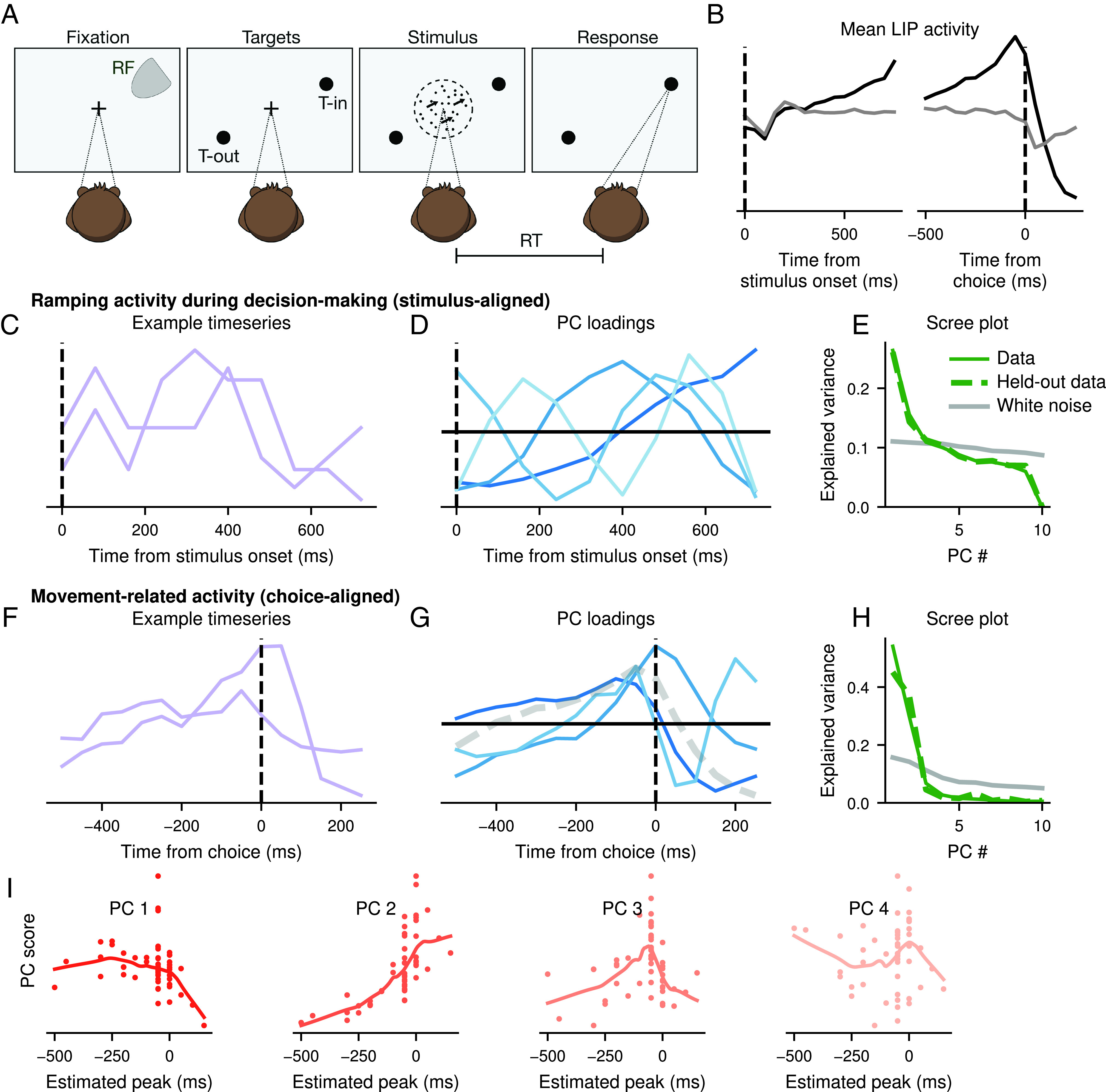
Phantom oscillations in the random dot motion task Roitman and Shadlen (33) recorded from LIP in monkeys performing a decision-making task. (A) Diagram of the experiment. (B) Mean activity for trials with a long response time (RT) (RT $>800$ ms) with a choice in the direction of T-IN (black) or T-OUT (gray). (C–E) Timeseries during decision-making period for long trials (RT $>800$ ms). (C) Two example timeseries during this period, representing individual trials. (D) PCA was performed on all trials and the PC loadings are shown. (E) PCA was recomputed on 1/2 of the trials. Variance explained is shown in solid green. The remaining 1/2 of trials were projected onto the loadings, and the variance explained by this projection is dashed green. Gray is the variance explained by the PCs of an equivalent-sized white noise dataset. (F–I) Timeseries during decision-making period for long trials (RT $>800$ ms). (F) Two example timeseries during this period, representing individual cells. (G) PCA was performed on all neurons and the PC loadings are shown. (H) PCA was recomputed on 2/3 of the neurons. Variance explained is shown in solid green. The remaining 1/3 of neurons were projected onto the loadings, and the variance explained by this projection is dashed green. Gray is the variance explained by the PCs of an equivalent-sized white noise dataset. (I) PC scores are plotted against the estimated peak of each neuron’s timeseries. LOESS-smoothed lines indicate the trend.

First, the activity of neurons in LIP leads to smoothness-driven phantom oscillations. Many neurons in LIP are known to reflect the accumulated information in favor of a choice toward T-IN (Fig. 4 B, Left) (33), often modeled using diffusion (34, 35). Diffusion produces smooth timeseries, and simulations of diffusion show phantom oscillations (SI Appendix, Fig. S1). Therefore, trial-by-trial neural activity aligned to the onset of the stimulus should show smoothness-driven phantom oscillations. We examine the first 700 ms of activity after the stimulus, using only trials at least 700 ms long (Fig. 4C). We find that the principal components of these data closely resemble sinusoidal oscillations (Fig. 4D). Using cross-validation, we fit data on a subset of 66% of the data and project the remaining 33% onto these PCs. The variance explained on the held-out data is similar to that of the training data, and much higher than for a white noise timeseries (Fig. 4E). Therefore, phantom oscillations are present in neural activity traditionally considered to be diffusion-like.

Second, bursts of activity in response to eye movements lead to shift-driven phantom oscillations. Many neurons in LIP show sharp increases in activity during eye movements toward T-IN (Fig. 4 B, Right). Furthermore, these bursts of activity are unlikely to show exactly the same peak timing in each neuron (Fig. 4F). Therefore, the mean activity of cells should show shift-driven phantom oscillations. Indeed, we find that the principal components resemble the derivatives of the mean (Fig. 4G). When PCA is performed on 66% of data and the remaining 33% are projected onto the PCs, a similar amount of variance is explained in the training and held-out data, much higher than for a white noise timeseries (Fig. 4H). Furthermore, the scores of these first principal components correlate with the peak of the timeseries, an estimate of the shift (Fig. 4I). Therefore, both smoothness-driven and shift-driven phantom oscillations are present in different aspects of the same decision-making experiment. This dataset is also relatively small by modern standards, containing only 54 neurons, demonstrating that phantom oscillations are not limited to big data.

Detecting True Oscillations in Data.

If oscillations are observed in PCA, how can we determine whether they are true oscillations or phantom oscillations? In general, PCA is not well suited to detecting oscillations, so most oscillations tend to be phantom oscillations. Distinguishing true oscillations from phantom oscillations is not always possible; for example, if only one cycle of the oscillation is present, true oscillations are impossible to identify on both on a technical and a conceptual level. Nevertheless, for cases where true oscillations may exist, we present three strategies to distinguish them from phantom oscillations.

To demonstrate these strategies, we analyze experimental data containing true oscillations for comparison to the phantom oscillations observed above. Ames and Churchland (36) instructed monkeys to travel through a linear virtual reality environment by moving a manipulandum in a cyclic pedaling motion (Fig. 5A). The distance the monkey needed to travel in virtual reality was fixed and corresponded to seven pedals on the manipulandum. While the monkeys performed the task, multiple neurons in the motor cortex were recorded simultaneously. Consistent with Ames and Churchland (36), we discarded first cycle and last two cycles to maintain a steady state cycling motion, rescaling the remaining four cycles to a 2 s interval for analysis (Fig. 5B). This means that the arm movements on each trial were exactly 2 hz, with the same phase at each timepoint in all trials.

Fig. 5.

True oscillations in a pedal task. Ames and Churchland (36) recorded from the motor cortex in monkeys performing a pedaling task. (A) Diagram of the experiment, reproduced from ref. 36. (B) Horizontal and vertical positions of the arm during the pedaling task during an example trial. Only the middle four cycles were analyzed. Cycles were rescaled in this period to allow averaging across trials by arm position. (C) Mean activity of three example neurons during the analyzed time period. (D) PCA was performed on the mean activity of each neuron during the task, and the loadings are shown. (E) PCA was recomputed on half of the neurons, and the variance explained is shown in green (solid). The remaining neurons were projected onto the PCs from the first half, and the variance explained is shown in green (dashed). For comparison, PCA was performed on an equal number of white noise timeseries of the same length, and variance explained is shown in gray. (F–H) Measures for detecting phantom oscillations are shown for the pedal task, a dataset with true oscillations (Left) as well as the other datasets exhibiting smoothness-driven and shift-driven phantom oscillations we have seen so far. (F) The power spectrum from the pedal task. (G) The covariance matrices for each of these datasets. (H) For each dataset, the number of oscillations (i.e., the wave number) for each PC loading is shown.

As reported by Ames and Churchland (36), these arm movements led to regular 2-hz firing patterns in neurons from the motor cortex. Most of the neurons showed an oscillation with 2 hz periodicity, and these neurons had diverse waveforms and phase offsets (Fig. 5C, light purple). Due to this diversity of phases and waveforms, there was little evidence of synchronized oscillatory activity in the mean neuron activity (Fig. 5C, dark purple). After computing PCA, we saw that the second and third principal components resembled sinusoidal oscillations at 2 hz (Fig. 5D) and explained a large fraction of variance, even after cross-validation (Fig. 5E). These two components were separated by a 90° phase, so linear combinations could capture a 2-hz sinusoidal oscillation of any phase. Given the 2-hz oscillations of the arm movements and 2-hz oscillations of the neurons, the 2-hz oscillations in the PCs appear to reflect true 2-hz oscillations in the data. We will demonstrate this below by comparing these PCs of putative true oscillations to our previous examples of phantom oscillations from smooth (Fig. 2) and time-shifted (Fig. 3) simulations, resting state fMRI (Fig. 2), and the random dot motion task Fig. 4.

One strategy to identify true oscillations is to use traditional methods for detecting oscillations in timeseries, such as peaks in the power spectrum. True oscillations will often appear as distinct peaks in the power spectrum, whereas phantom oscillations always appear as a $1/f$-like pattern which decreases with increasing frequency. This $1/f$-like pattern has been previously characterized as the “aperiodic” part of the spectrum (37). While power spectra may contain false peaks due to windowing effects, harmonics, and other artifacts, the absence of peaks in the power spectrum is strong evidence that an oscillation is actually a phantom oscillation. We compute the power spectrum as the mean spectrum of all timeseries in our data. In our cycling dataset, we see a clear peak in the power spectrum at 2 hz corresponding to the four cycles of the manipulandum, as well as a peak at 4 hz corresponding to the first harmonic (Fig. 5 F, Left). By contrast, no such peaks are present in the power spectrum for the other datasets (Fig. 5F).

A second strategy to identify true oscillations is to inspect the covariance matrix. In phantom oscillations, we expect one thick prominent stripe along the diagonal of the matrix, covering either all (SI Appendix, Fig. S1) or part (SI Appendix, Fig. S6) of the diagonal. By contrast, for true oscillations, we expect multiple diagonal stripes throughout the covariance matrix. These multiple stripes represent the correlation across different phases of the same oscillation. We observe multiple stripes in the pedaling dataset (Fig. 5 G, Left), but only one thick stripe in the others (Fig. 5G).

A third strategy is based on the fact that a single phantom oscillation principal component is never found alone. Phantom oscillations always appear across many frequencies, often with a distinct frequency in each principal component. Smoothness-driven phantom oscillations with low oscillatory frequency will explain more variance than those with higher frequency, and shift-driven phantom oscillations tend to follow a similar pattern as well. The slope of this relationship should increase consistently with a slope less than 1, linearly or step-wise, and should not make any large jumps. Therefore, the oscillation frequency will form a monotonic relationship with the ordering of the PCs. In the simulated, fMRI, and decision-making data, we see a near-linear relationship between the PC number and the frequency of the oscillation (Fig. 5H). By contrast, in the cycling data, after a first constant PC, the second and third PCs oscillate four times, and the fifth and sixth oscillate 8 times (Fig. 5H, Left).

Putative shift-driven phantom oscillations have an additional property which distinguishes them from true oscillations. As we saw previously (Fig. 3 E and F) (Fig. 4I), the PC scores of shift-driven phantom oscillations are correlated with the magnitude of the shift. Performing this analysis requires estimating a time shift from each observation, using methods including cross-correlation, peak detection, or other techniques. Since the relationship may be nonmonotonic, a Pearson correlation may be insufficient, but examining this relationship by eye should provide an indication of nonlinear relationships. Therefore, several strategies can be used to determine whether an oscillation is a phantom oscillation or a true oscillatory signal.

Discussion

Despite being one of the simplest forms of dimensionality reduction, PCA’s interpretation can be complicated. Here, we showed that PCs may exhibit oscillations that do not exist in the underlying data. This is because real-life data often vary along a continuum—such as time in a timeseries, or position in spatially embedded data. However, data that vary along a continuum violate the implicit assumptions underlying the classic interpretation of PCA. Other examples of continua include neurons along a linear probe, subjects in a longitudinal experiment, or brain regions in an imaging experiment. We showed that there are two distinct ways that phantom oscillations can arise from a continuum: smoothness, and shifts across observations. Our simulations and data analysis showed different patterns for smoothness-driven and shift-driven phantom oscillations. Likewise, in SI Appendix, we determined that smoothness is related to the second derivative of the timeseries, whereas shifts are related to the first derivative. We also provided a simple method to test for both types of phantom oscillations. Our results may apply more broadly to topographic space, such as place cells (38), retinotopy and tonotopy, or concepts in high-dimensional space defined across a graph.

We are not the first to observe phantom oscillations. Previous work found similar oscillations from PCA in neural data (22) and tuning curves (39), as well as other types of smooth data, such as natural images (18, 40), music (41), and spatial population genetics (19). In one notable example, several authors showed that the oscillation-like activity observed in the motor cortex during reaching (4) could be traced to an artifact of dimensionality reduction (21, 22, 42). Phantom oscillations also resemble the oscillation modes in whole brain imaging experiments (28–31), which is connected to PCA through the same set of differential equations (SI Appendix). We (SI Appendix, Fig. S3) and others (22) showed that, when plotted against each other, phantom oscillations can show a U-shape. This effect, also known as the “horseshoe effect,” is also found in other dimensionality reduction methods such as multidimensional scaling (MDS) (43, 44). Nevertheless, in SI Appendix, we show that phantom oscillations are more complicated than simply the terms of a Fourier series. This is because phantom oscillations often have noninteger and nonuniformly spaced oscillatory frequencies. Additionally, phantom oscillations may only produce one sinusoid at each frequency, whereas a Fourier series requires a sine and a cosine at each frequency to account for phase shifts. The only condition in which phantom oscillations do resemble a Fourier series is the rare situation when the edges of the timeseries wrap around, such that the first and last points are correlated with each other in the same way as neighboring points. This results in a “step-like” scree plot (SI Appendix and SI Appendix, Fig. S1).

The conditions that cause phantom oscillations are ubiquitous in neuroscience data. Smoothness may occur for biological or methodological reasons. On the biological side, reasons include slow intrinsic neural and circuit time constants and the fact that behavior is often history-dependent. On the methodological side, reasons include measurements of activity with slow dynamics, such as calcium indicators or the hemodynamic response function in fMRI. More generally, any type of low-pass filtering makes data vulnerable to phantom oscillations. Shifts may also occur for biological or methodological reasons. On the biological side, different subjects or neurons may have slight intrinsic differences in response time. Response time may also vary across trials within a subject, or may depend on external factors like attention or arousal (45). There also may be multiple points of interest, such as the stimulus and choice onsets in our decision-making dataset, making it difficult or impossible to align to both. On the methodological side, a slow sampling rate or imprecision in alignment may create the same effect. Additionally, volumetric imaging technologies such as two-photon imaging or fMRI usually acquire volumetric planes sequentially, leading to shifts in timing across planes. In most cases of shift-driven phantom oscillations, data must be aligned to an external signal or reference registration, so realignment is not an option.

It remains to be shown whether it is possible to compute PCA in a way which is robust to phantom oscillations. One potential approach for smoothness-driven phantom oscillations is to formulate an appropriate noise model. For instance, in factor analysis and probabilistic PCA (PPCA), there is an explicit model of the noise (46) which assumes noise is independent and normally distributed (47). Using a correlated noise model to account for smoothness may help reduce the effect of smoothness-driven phantom oscillations. Such a noise model may help to bring out true underlying patterns even in data which do not show phantom oscillations. For example, true oscillations were found in the Ames and Churchland data, but these data also contained neurons which were naturally smooth, and artificial smoothing was applied during preprocessing. Had this smoothness been accounted for by an appropriate noise model, the true oscillations identified by PCA may have been even stronger.

PCA is often used as a way to compare brain activity across different experimental conditions. However, if differences in PCs are observed when phantom oscillations are present, these differences may be a proxy for some simpler phenomenon. For example, since the PC score is correlated with the location of the peak in shift-driven phantom oscillations, any change in the peak latency across conditions will be reflected in the PCs. Moreover, anything which is correlated with this latency will also be correlated with the PC score. In smoothness-driven phantom oscillations, differences in smoothness across observations will also be reflected in the PCs. Such differences may arise from many sources, including variation in firing rate or signal-to-noise ratio. Therefore, in the presence of phantom oscillations, group differences in PC loadings or scores can often be explained by a simpler statistical property of the data.

Phantom oscillations are an artifact of dimensionality reduction and should not be interpreted. The exact form of phantom oscillations is determined by a complex nonlinear combination of factors such as the smoothness, the distribution of shifts, the distribution of variance, and the behavior at the edges. These factors can all be measured without relying on phantom oscillations. Additionally, the form of phantom oscillations is sensitive to small differences in the data, such as adding a constant. It can also be insensitive to large changes; for example, all data with homogeneous smoothness that wrap around have identical principal components. We provided intuitions for how these different cases behave in SI Appendix, Figs. S1 and S6 and SI Appendix. On a similar note, PCA is not the ideal tool to study true oscillations. PCA can fail to identify true oscillations, such as those that are phase-locked, and it struggles to identify multiple oscillatory frequencies simultaneously. Specialized tools should be used for detecting oscillations (37).

In this work, we focused on the case where time is the feature dimension, and thus, the loadings represent points in time. By contrast, in neuroscience, it is common to perform PCA with time in the observation dimension, which is equivalent to performing PCA of the transpose of the data matrix. We focus on the former for three reasons. First, performing PCA along the feature dimension allows us to assume our observations are independent samples from the same statistical process. The standard interpretation of PCA, where components represent latent patterns in the data, assumes that observations are independent. If smoothness occurred in the observation dimension, then the observations would by definition no longer be independent. Our mathematical analyses are largely based on the Karhunen-Loève transform, which also assumes observations are independent. Second, the relationship between the covariance matrix and smoothness is only visually evident as a thick diagonal when smoothness occurs in the feature dimension. It may be possible to rearrange the rows and columns of the covariance matrix to emphasize this thick diagonal, but this is beyond the scope of most analyses. Third, PCA along the observation dimension gives very similar results to PCA across the feature dimension. We showed that, in our simulations, both smoothness and time shifts cause oscillations regardless of whether the smoothness or time shifts are in the feature or observation dimension. We also provided a mathematical justification for why this is the case in SI Appendix. Therefore, phantom oscillations occur no matter the dimension that PCA is performed.

PCA is closely related to many other forms of dimensionality reduction. For example, our mathematical analyses can be applied almost identically to SVD, which is the same method as PCA except without mean subtraction. Additionally, phantom oscillations have been reported for other forms of dimensionality reduction, including demixed PCA (48), jPCA (21), and MDS (43, 44). These methods involve finding the eigenvectors of a matrix multiplied by its transpose, such as a covariance matrix, correlation matrix, or matrix of second moments. It remains to be shown whether phantom oscillations or other biases occur in dimensionality reduction methods that are conceptually similar but mathematically different from PCA, such as factor analysis (FA), nonnegative matrix factorization (NMF), or independent component analysis (ICA). For example, subsequence timeseries clustering does not utilize eigenvectors but still shows phantom oscillations (49). It is also unknown how phantom oscillations impact other machine learning methods that use PCA for preprocessing. Many studies explore how low-level statistics influence dimensionality reduction (21–23, 32, 50–58). These studies mirror our own by showing that patterns in high-dimensional data analysis may not always reflect true patterns in the data.

Materials and Methods

A. Mathematical Explanations, Derivations, and Proofs.

Mathematical details can be found in SI Appendix. In brief, we prove that both smoothness and shifts cause phantom oscillations. For smooth data, we show how PCA is linked to the differential equation for a harmonic oscillator. We also compute closed-form expressions for PCs using the Karhunen-Loève transform. For shifted data, we show why the derivatives of the shifted signal can be used to construct the PCs. Mathematical proofs are accompanied by intuitive explanations.

B. Smoothness-Driven Phantom Oscillations.

The smooth artificial timeseries were generated as smoothed white noise. We generated 100,000 artificial timeseries of length 300 drawn from the standard normal distribution. We filtered with a Gaussian filter of SD 4. We discarded all but the central 60 timepoints to avoid edge effects of the filtering, leaving 100,000 timeseries of length 60. We repeated this procedure to create an equally sized dataset for cross-validation.

The resting state fMRI data were derived from the Cam-CAN project (26). We used the resting state scans with the AAL parcellation, as provided by the Cam-CAN project. To remove transient high-frequency artifacts, we applied a low-pass Butterworth filter at half the Nyquist frequency. For each of the 646 subjects, we selected 60 parcels with replacement, and for each selection, we chose a random segment of 60 time points. Sampling rate (TR) was 1.97 s, for a total of 118.2 s of data. In total, this yielded 38,760 timeseries. We randomly selected half of these, 19,380, for our core dataset, and used the rest for cross-validation.

The spatially smooth data were generated by drawing from a multivariate normal distribution. Each timepoint was one sample from this distribution. The covariance matrix was determined as negative exponential of distance for each region or pixel. For the data in the geometry of a widefield recording, we drew 10,000 independent samples of size 5,916 (for 5,916 pixels in the image) and for the geometry of cortex, 3,000 independent samples of size 180 (for 180 pixels in the parcellation of ref. 59.

C. Shift-Driven Phantom Oscillations.

The random shifts in timing data were generated based on the response of frontal eye field neurons to a delayed stimulus (60). The base timeseries was taken from the freely available data provided by ref. 60, using the mean activity from cells in Monkey Q with 70% coherence in the 400-ms presample condition, with data from 600 ms before and after stimulus onset with 10 ms time bins. The resulting timeseries was smoothed with a Savitzky–Golay filter of order 1 with a window length of 5. We drew 2,000 time shift offsets from a uniform distribution from 0.1 to 0.4. The base timeseries was upsampled through linear interpolation according to each shift, and the segment from 0 to 700 ms was selected. This yielded 2,000 timeseries of length 700. We repeated this sampling and interpolation process to create another 2,000 timeseries to be used for cross-validation only.

The random shifts with nonidentical signals were generated using noisy difference of gammas. We generated base data using

$$x_i(t)=f_3(t-2{\mathrm{\Delta }}_i)-(s_i/3+0.4)f_{3b_i+4}(t-2{\mathrm{\Delta }}_i)+0.03w_i(t-2{\mathrm{\Delta }}_i),$$

where ${\mathrm{\Delta }}_i\sim U[0,1]$ is the shift in time, $b\sim U[0,1]$ is the shape parameter, $s_i\sim U[0,1]$ is the amplitude of the second gamma for timeseries $i$, $f_k(t)$ is the probability density function of the gamma distribution with shape parameter $k$, and $w_i(t)$ is $1/f^{\alpha }$ noise with exponent 1.8. We chose this form arbitrarily because it visually approximates a noisy hemodynamic response function. We generated 2,000 timeseries of length 10 s at 100 hz this way, and 2,000 additional timeseries for cross-validation only.

The images were generated with a single static two-photon image of two neurons. The shifts for the image were computed by filtering a white noise timeseries of length 10,000 with a Gaussian filter of SD 5. Only a small segment of this timeseries is shown in (Fig. 3G). Shifts were applied to the image, simulating movement of the imaging window, and images were flattened before computing PCA.

D. Random Dot Motion Task.

Full details of the random dot motion experiment are described in ref. 33. Due to the limited number of neurons recorded in this dataset, analyses presented here pool data from both monkeys. For illustration purposes, in the schematic Fig. 4B, we used neural activity averaged across all trials with an RT greater than 800 ms, with a bin size of 50 ms.

For our analysis of diffusion-like activity showing smoothness-driven phantom oscillations, we examined the period from 0 to 800 ms after the onset of the stimulus, using a bin size of 80 ms. We restricted to trials which had an RT greater than 800 ms. This gave a total of 1,821 trials with 10 time points per trial.

For our analysis of transient activity showing shift-driven phantom oscillations, we examined the period 500 ms before the saccade to 300 ms after the saccade, with a time bin of 50 ms. Because these transients generally occur when the target is in the receptive field, we only examined saccades to T-IN. To ensure a strong transient, we only considered trials with a motion coherence greater than 10%. Assuming each cell had a similar delay, we averaged the response of each neuron, for a total of 54 timeseries (one for each neuron) with 16 timepoints.

E. Pedal Task.

Full details of the pedal experiment are described in ref. 36. We used data only from monkey E, starting from the top, pedaling in the forward direction with both hands. Activity was averaged for each neuron, and all sessions were pooled for a total of 626 neurons. While pedaling on each trial was performed at approximately the same speed, it was not exactly the same on each trial. Therefore, to find average firing rate for each neuron at each point in time, trials were aligned according to the pedal position, and this was rescaled across time such that each cycle took 500 ms. Data were slightly smoothed with a 25-ms Gaussian filter to compute an instantaneous firing rate and allow for this rescaling. The first two cycles and the last cycle were discarded. The hand position example in Fig. 5B uses the hand position of an example aligned trial.

Supplementary Material

Appendix 01 (PDF)

Data, Materials, and Software Availability

Previously published data were used for this work (26, 33, 36).

References

- 1.Pearson K., LIII. On lines and planes of closest fit to systems of points in space. London Edinb. Dublin Philos. Maga. J. Sci. 2, 559–572 (1901). [Google Scholar]
- 2.Hotelling H., Analysis of a complex of statistical variables into principal components. J. Ed. Psychol. 24, 417–441 (1933). [Google Scholar]
- 3.Russo A. A., et al. , Motor cortex embeds muscle-like commands in an untangled population response. Neuron 97, 953–966.e8 (2018). [DOI] [PMC free article] [PubMed] [Google Scholar]
- 4.Churchland M. M., et al. , Neural population dynamics during reaching. Nature 487, 51–56 (2012). [DOI] [PMC free article] [PubMed] [Google Scholar]
- 5.Rossi-Pool R., et al. , Decoding a decision process in the neuronal population of dorsal premotor cortex. Neuron 96, 1432–1446.e7 (2017). [DOI] [PubMed] [Google Scholar]
- 6.Rossi-Pool R., et al. , Temporal signals underlying a cognitive process in the dorsal premotor cortex. Proc. Natl. Acad. Sci. U.S.A. 116, 7523–7532 (2019). [DOI] [PMC free article] [PubMed] [Google Scholar]
- 7.N. A. Steinemann et al., Direct observation of the neural computations underlying a single decision. bioRxiv (2022). https://www.biorxiv.org/content/10.1101/2022.05.02.490321v1 (Accessed 3 August 2023).
- 8.Mante V., Sussillo D., Shenoy K. V., Newsome W. T., Context-dependent computation by recurrent dynamics in prefrontal cortex. Nature 503, 78–84 (2013). [DOI] [PMC free article] [PubMed] [Google Scholar]
- 9.Murray J. D., et al. , Stable population coding for working memory coexists with heterogeneous neural dynamics in prefrontal cortex. Proc. Natl. Acad. Sci. U.S.A. 114, 394–399 (2016). [DOI] [PMC free article] [PubMed] [Google Scholar]
- 10.Remington E. D., Narain D., Hosseini E. A., Jazayeri M., Flexible sensorimotor computations through rapid reconfiguration of cortical dynamics. Neuron 98, 1005–1019.e5 (2018). [DOI] [PMC free article] [PubMed] [Google Scholar]
- 11.Goudar V., Peysakhovich B., Freedman D. J., Buffalo E. A., Wang X. J., Schema formation in a neural population subspace underlies learning-to-learn in flexible sensorimotor problem-solving. Nat. Neurosci. 26, 879–890 (2023). [DOI] [PMC free article] [PubMed] [Google Scholar]
- 12.K. Jurewicz, B. J. Sleezer, P. S. Mehta, B. Y. Hayden, R. B. Ebitz, Irrational choices via a curvilinear representational geometry for value. bioRxiv (2022). https://www.biorxiv.org/content/10.1101/2022.03.31.486635v1.full (Accessed 1 April 2022). [DOI] [PMC free article] [PubMed]
- 13.Coenen A., Zayachkivska O., Adolf Beck: A pioneer in electroencephalography in between Richard Caton and Hans Berger. Adv. Cognit. Psychol. 9, 216–221 (2013). [DOI] [PMC free article] [PubMed] [Google Scholar]
- 14.Harding G., The Psychological Significance of the Electroencephalogram (Applied Psychology Department, University of Aston in Birmingham, 1968). [Google Scholar]
- 15.Bossomaier T., Snyder A. W., Why spatial frequency processing in the visual cortex? Vis. Res. 26, 1307–1309 (1986). [DOI] [PubMed] [Google Scholar]
- 16.Buzsáki G., Rhythms of the Brain (Oxford University Press, 2006). [Google Scholar]
- 17.Sato T. K., Nauhaus I., Carandini M., Traveling waves in visual cortex. Neuron 75, 218–229 (2012). [DOI] [PubMed] [Google Scholar]
- 18.Hancock P. J. B., Baddeley R. J., Smith L. S., The principal components of natural images. Netw.: Comput. Neural Syst. 3, 61–70 (1992). [Google Scholar]
- 19.Novembre J., Stephens M., Interpreting principal component analyses of spatial population genetic variation. Nat. Genet. 40, 646–649 (2008). [DOI] [PMC free article] [PubMed] [Google Scholar]
- 20.J. Antognini, J. Sohl-Dickstein, “PCA of high dimensional random walks with comparison to neural network training” in Advances in Neural Information Processing Systems, S. Bengio et al., Eds. (Curran Associates, Inc., 2018), vol. 31.
- 21.Lebedev M. A., et al. , Analysis of neuronal ensemble activity reveals the pitfalls and shortcomings of rotation dynamics. Sci. Rep. 9, 18978 (2019). [DOI] [PMC free article] [PubMed] [Google Scholar]
- 22.T. Proix, M. G. Perich, T. Milekovic, Interpreting dynamics of neural activity after dimensionality reduction. bioRxiv (2022). https://www.biorxiv.org/content/10.1101/2022.03.04.482986v1 (Accessed 24 April 2023).
- 23.De A., Chaudhuri R., Common population codes produce extremely nonlinear neural manifolds. Proc. Natl. Acad. Sci. U.S.A. 120, e2305853120 (2023). [DOI] [PMC free article] [PubMed] [Google Scholar]
- 24.Jolliffe I. T., Principal Component Analysis (Springer Nature, 2002). [Google Scholar]
- 25.N. Vaswani, H. Guo, “Correlated-PCA: Principal components analysis when data and noise are correlated” in Advances in Neural Information Processing Systems, D. Lee, M. Sugiyama, U. Luxburg, I. Guyon, R. Garnett Eds. (Curran Associates, Inc., 2016), vol. 29.
- 26.Shafto M. A., et al. , The Cambridge centre for ageing and neuroscience (cam-CAN) study protocol: A cross-sectional, lifespan, multidisciplinary examination of healthy cognitive ageing. BMC Neurol. 14, 204 (2014). [DOI] [PMC free article] [PubMed] [Google Scholar]
- 27.Kac M., Can one hear the shape of a drum? Am. Math. Mon. 73, 1–23 (1966). [Google Scholar]
- 28.Pang J. C., et al. , Geometric constraints on human brain function. Nature 618, 566–574 (2023). [DOI] [PMC free article] [PubMed] [Google Scholar]
- 29.Robinson P., et al. , Eigenmodes of brain activity: Neural field theory predictions and comparison with experiment. NeuroImage 142, 79–98 (2016). [DOI] [PubMed] [Google Scholar]
- 30.Bolt T., et al. , A parsimonious description of global functional brain organization in three spatiotemporal patterns. Nat. Neurosci. 25, 1093–1103 (2022). [DOI] [PubMed] [Google Scholar]
- 31.Atasoy S., Donnelly I., Pearson J., Human brain networks function in connectome-specific harmonic waves. Nat. Commun. 7, 10340 (2016). [DOI] [PMC free article] [PubMed] [Google Scholar]
- 32.Watson D. M., Andrews T. J., Connectopic mapping techniques do not reflect functional gradients in the brain. NeuroImage 277, 120228 (2023). [DOI] [PubMed] [Google Scholar]
- 33.Roitman J. D., Shadlen M. N., Response of neurons in the lateral intraparietal area during a combined visual discrimination reaction time task. J. Neurosci. 22, 9475–9489 (2002). [DOI] [PMC free article] [PubMed] [Google Scholar]
- 34.Ratcliff R., McKoon G., The diffusion decision model: Theory and data for two-choice decision tasks. Neural Comput. 20, 873–922 (2008). [DOI] [PMC free article] [PubMed] [Google Scholar]
- 35.Shinn M., Lam N. H., Murray J. D., A flexible framework for simulating and fitting generalized drift-diffusion models. eLife, 9 (2020). [DOI] [PMC free article] [PubMed]
- 36.Ames K. C., Churchland M. M., Motor cortex signals for each arm are mixed across hemispheres and neurons yet partitioned within the population response. eLife 8, e46159 (2019). [DOI] [PMC free article] [PubMed] [Google Scholar]
- 37.Donoghue T., et al. , Parameterizing neural power spectra into periodic and aperiodic components. Nat. Neurosci. 23, 1655–1665 (2020). [DOI] [PMC free article] [PubMed] [Google Scholar]
- 38.Dordek Y., Soudry D., Meir R., Derdikman D., Extracting grid cell characteristics from place cell inputs using non-negative principal component analysis. eLife 5, e10094 (2016). [DOI] [PMC free article] [PubMed] [Google Scholar]
- 39.Zhu R. J. B., Wei X. X., Unsupervised approach to decomposing neural tuning variability. Nat. Commun. 14, 2298 (2023). [DOI] [PMC free article] [PubMed] [Google Scholar]
- 40.Olshausen B. A., Field D. J., Emergence of simple-cell receptive field properties by learning a sparse code for natural images. Nature 381, 607–609 (1996). [DOI] [PubMed] [Google Scholar]
- 41.B. Cornelissen, W. Zuidema, J. A. Burgoyne, “Cosine contours: A multipurpose representation for melodies” in Proceedings of 22th International Conference Music Information Retrieval (2021).
- 42.Michaels J. A., Dann B., Scherberger H., Neural population dynamics during reaching are better explained by a dynamical system than representational tuning. PLoS Comput. Biol. 12, e1005175 (2016). [DOI] [PMC free article] [PubMed] [Google Scholar]
- 43.Kendall D. G., A mathematical approach to seriation. Philos. Trans. R. Soc. London. Ser. A Math. Phys. Sci. 269, 125–134 (1970). [Google Scholar]
- 44.Diaconis P., Goel S., Holmes S., Horseshoes in multidimensional scaling and local kernel methods. Ann. Appl. Stat. 2, 777–807 (2008). [Google Scholar]
- 45.Luce R. D., Response Times: Their Role in Inferring Elementary Mental Organization (Oxford University Press, 1986). [Google Scholar]
- 46.Cunningham J. P., Yu B. M., Dimensionality reduction for large-scale neural recordings. Nat. Neurosci. 17, 1500–1509 (2014). [DOI] [PMC free article] [PubMed] [Google Scholar]
- 47.Tipping M. E., Bishop C. M., Probabilistic principal component analysis. J. R. Stat. Soc.: Ser. B (Stat. Methodol.) 61, 611–622 (1999). [Google Scholar]
- 48.Kobak D., et al. , Demixed principal component analysis of neural population data. eLife 5, e10989 (2016). [DOI] [PMC free article] [PubMed] [Google Scholar]
- 49.Keogh E., Lin J., Clustering of time-series subsequences is meaningless: Implications for previous and future research. Knowl. Inf. Syst. 8, 154–177 (2005). [Google Scholar]
- 50.M. Helmer et al., On stability of Canonical Correlation Analysis and Partial Least Squares with application to brain-behavior associations. bioRxiv (2023). https://www.biorxiv.org/content/10.1101/2020.08.25.265546v4 (Accessed 27 April 2023). [DOI] [PMC free article] [PubMed]
- 51.K. D. Harris, Nonsense correlations in neuroscience. bioRxiv (2020). https://www.biorxiv.org/content/10.1101/2020.11.29.402719v3 (Accessed 19 June 2021).
- 52.Shinn M., et al. , Functional brain networks reflect spatial and temporal autocorrelation. Nat. Neurosci. 26, 867–878 (2023). [DOI] [PubMed] [Google Scholar]
- 53.Elsayed G. F., Cunningham J. P., Structure in neural population recordings: An expected byproduct of simpler phenomena? Nat. Neurosci. 20, 1310–1318 (2017). [DOI] [PMC free article] [PubMed] [Google Scholar]
- 54.Burt J. B., Helmer M., Shinn M., Anticevic A., Murray J. D., Generative modeling of brain maps with spatial autocorrelation. NeuroImage 220, 117038 (2020). [DOI] [PubMed] [Google Scholar]
- 55.Schultze S., Grubmüller H., Time-lagged independent component analysis of random walks and protein dynamics. J. Chem. Theory Comput. 17, 5766–5776 (2021). [DOI] [PMC free article] [PubMed] [Google Scholar]
- 56.Moore J., Ahmed H., Antia R., High dimensional random walks can appear low dimensional: Application to influenza H3N2 evolution. J. Theor. Biol. 447, 56–64 (2018). [DOI] [PMC free article] [PubMed] [Google Scholar]
- 57.Perrenoud Q., Cardin J. A., Beyond rhythm – A framework for understanding the frequency spectrum of neural activity. Front. Syst. Neurosci. 17, 1217170 (2023). [DOI] [PMC free article] [PubMed] [Google Scholar]
- 58.Chari T., Pachter L., The specious art of single-cell genomics. PLoS Comput. Biol. 19, e1011288 (2023). [DOI] [PMC free article] [PubMed] [Google Scholar]
- 59.Glasser M. F., et al. , A multi-modal parcellation of human cerebral cortex. Nature 536, 171–178 (2016). [DOI] [PMC free article] [PubMed] [Google Scholar]
- 60.Shinn M., Lee D., Murray J. D., Seo H., Transient neuronal suppression for exploitation of new sensory evidence. Nat. Commun. 13 (2022). [DOI] [PMC free article] [PubMed] [Google Scholar]
Associated Data
This section collects any data citations, data availability statements, or supplementary materials included in this article.
Supplementary Materials