Zoning and affordability: A reply to Rodríguez-Pose and Storper

Abstract

Would increasing allowable housing densities in expensive cities generate more housing construction and make housing more affordable? In a provocative article, Andrés Rodríguez-Pose and Michael Storper survey the evidence and answer no. Restrictions on housing density, they contend, do not substantially influence housing production or price. They further argue that allowing more density in growing metropolitan areas would only improve housing outcomes for the affluent, and most likely harm the poor. We take issue with both of these contentions. While uncertainties remain in the study of housing prices and land use regulation, neither theory nor evidence warrant dispensing with zoning reform, or concluding that it could only be regressive. Viewed in full, the evidence suggests that increasing allowable housing densities is an important part of housing affordability in expensive regions.

Introduction

Would relaxing zoning regulations in expensive cities encourage more housing construction and make housing more affordable? Andrés Rodríguez-Pose and Michael Storper (2020) (R-S), in their article ‘Housing, urban growth and inequalities: The limits to deregulation and upzoning in reducing economic and spatial inequality’, survey the evidence and say no. In making this argument, they position themselves against what they call the ‘Housing as Opportunity’ school of thought, which in their telling has come to ‘dominate’ academic discussions about housing affordability. Housing as Opportunity scholars, to R-S, are overly focused on zoning, and blind to the fact that land use restrictions have little relationship to housing prices or affordability. ‘The affordability crisis is real’, R-S write, but it is ‘due less to over-regulation of housing markets than to the underlying wage and income inequalities, and a sharp increase in the value of central locations within metro areas, as employment and amenities concentrate in these places’ (Rodríguez-Pose and Storper, 2020: 225).

What should we make of this argument? ‘Housing, urban growth and inequalities’ is an article with a lot going on in it, and a lot going on around it. R-S spend much of the article discussing interregional migration, because they disagree with the idea that less regulation in prosperous regions would let those places grow, and thus increase the size of national economies. In a subpart of that discussion, they also attack a stream of economic literature that is sceptical of place-based efforts to revive declining regions. Yet another, albeit smaller, part of their argument asserts that the academic focus on affordability problems in prosperous regions has exacerbated feelings of neglect and discontent in places that are struggling, and has helped fuel the rise of political populism as a result.

R-S, in short, pick many fights. In most of these fights, we don’t have a dog. We are researchers interested in the relationship between regulation, housing supply and housing prices. Like Storper, we are involved in discussions and advocacy around these issues in our home state of California. So we do have a stake in the claims R-S build to and conclude with: that regulation does not meaningfully influence housing supply and prices, and changing zoning to increase supply would only help the affluent.

These latter claims also have the most policy relevance. The typical argument about zoning in California and other expensive places emphasises its relationship to housing prices (and to a lesser extent the environment). The idea that deregulation will make the national economy larger is sometimes mentioned, but plays a secondary role. Perhaps as a result, the claims about zoning and affordability earned the R-S article the most attention upon its release. The renowned urbanist Richard Florida devoted a prominent essay to the R-S article on Citylab, titled it ‘“Build more housing” is no match for inequality’, and wrote that, ‘a new analysis finds that liberalising zoning rules and building more won’t solve the urban affordability crisis, and could exacerbate it’ (Florida, 2019). Florida quoted Rodríguez-Pose that ‘Upzoning is far from the progressive policy tool it has been sold to be. It mainly leads to building high-end housing in desirable locations.’ Storper, meanwhile, in an interview about ‘Housing, urban growth and inequalities’ in California’s Planning Report, said ‘The idea that upzoning will cause affordability to trickle down in our metropolis is based on a narrative of housing as opportunity that is deeply flawed … Blanket upzoning is likely to miss its affordability target’ (Planning Report, 2019).

We disagree. In this response we explain why. R-S contend that zoning scholars like us should think more about the geography of labour, and about why some places are attracting so many people. They argue, in essence, that housing demand is the story, not housing supply. On some level this point is incontrovertible: San Francisco would be cheap, full stop, if it had no jobs and no one wanted to live there. Supply is immaterial in demand’s absence. But this point skirts the argument more than it wins it. The conventional view on zoning and affordability is an argument about supply conditional on demand: given that San Francisco’s economy is booming (and, by extension, that other places are lagging behind it), would the region be less expensive if it let more housing be built?

One can call this question unimportant – that is a matter of judgement. One can say the question is no more important than the question of how to revitalise places in decline. Certainly the distress of renters in San Francisco does not obviously supersede the distress of low-income people in Detroit. And it is entirely reasonable to say that more development would not by itself make expensive cities like San Francisco affordable to everyone. To our knowledge, no one contends as much. Virtually every academic supporter of upzoning considers it necessary but not sufficient. A strong role remains for low-income housing subsidies, and we support dramatic increases in such redistribution to low-income people.

R-S go beyond those points, however, and say that in expensive places more development will not help, and in fact could hurt, because supply plays little role in housing problems. Here, we think R-S fail to make their case. They show that high-income people move to expensive places, but never explain why removing existing restrictions on housebuilding in those places would not help absorb those people, and alleviate the pressure they put on prices.

In what follows we identify what we see as the shortcomings in the R-S argument. We first lay out the conventional wisdom that R-S are attacking. From there we examine the empirical case that R-S build against this thinking, and the literature they invoke. Lastly, we reflect more broadly on their underlying theory: what it would mean to have a housing market where supply played so little role?

A few points before proceeding. As we have noted, the R-S argument about zoning and affordability is woven, throughout their article, into their other arguments about migration and declining places. As a result, at times we present their points in an order different from how they appear in the original article (for example, we are going to show their Figure 6 before their Figure 3). We do this mainly for ease of exposition, and we try to be transparent about it. We think and hope that we do no disservice to the R-S argument by presenting it in this manner. Nevertheless, readers are encouraged to go to the original article and keep us honest.

Figure 3.

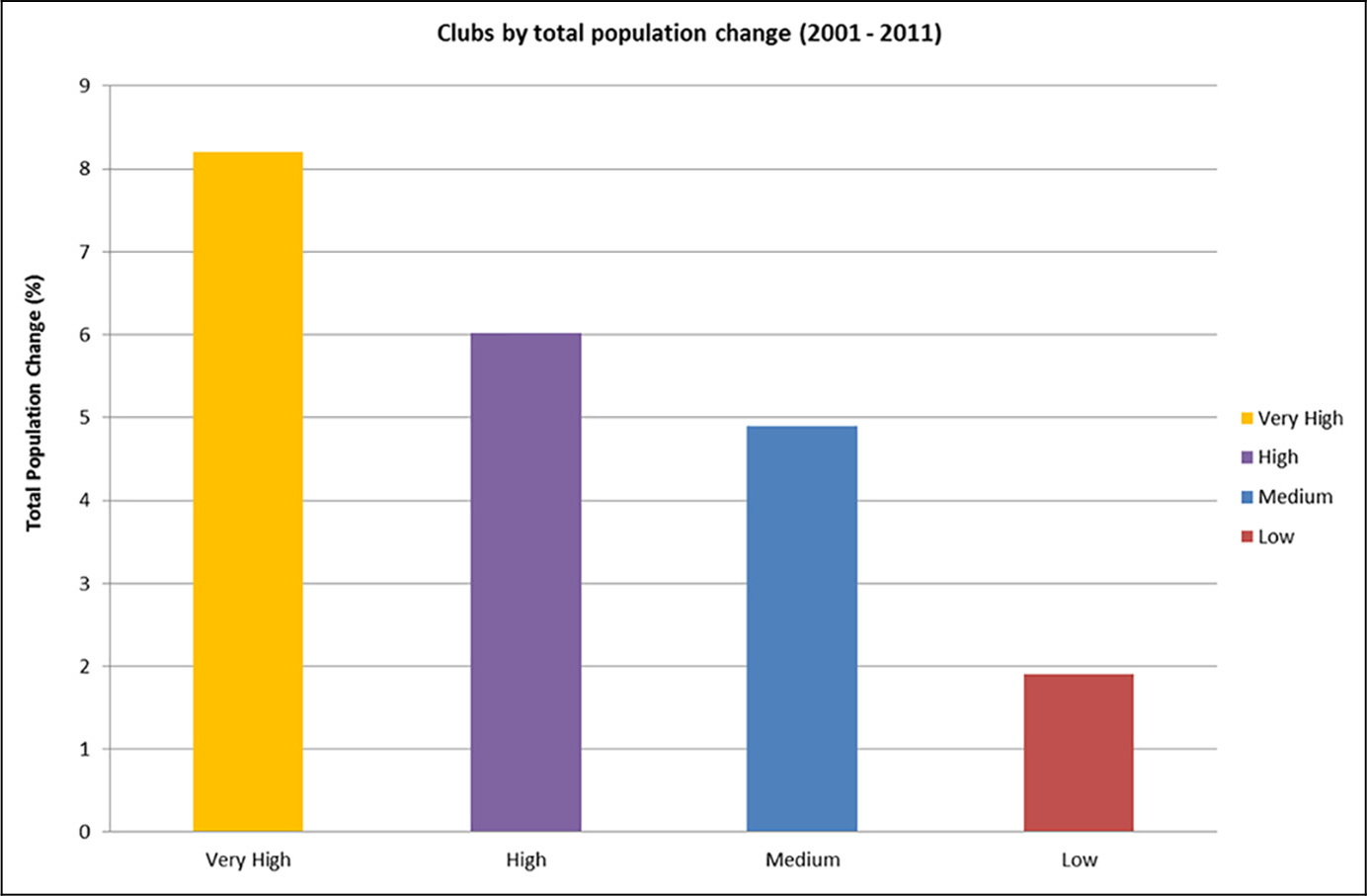
Population growth in European regions by income levels, 2001–2014.

Source: Reproduction of Figure 3 in Rodríguez-Pose and Storper (2020).

Also as we mentioned above, R-S make many arguments that we do not address. Readers should not interpret our silence as endorsement. Many of R-S’s arguments seem wrong to us. We disagree with their ideas about spatial equilibrium; we think they misrepresent the economic literature on place-based policy; and we see no clear causal path between concern about housing prices and the rise of reactionary politics. Most of all, we think they paint an inaccurate picture of academic housing research, falsely claiming that ‘serious’ affordability policies are ‘curiously absent’ from it. Space is limited, however, so we focus our attention on the zoning argument.

Zoning’s limited impact on prices?

To start everyone on the same page, we first present the conventional argument that regulation drives up housing prices. That argument is as follows. When a region’s economy grows, more people want to live there, to access its jobs, amenities and other opportunities. If this new demand for housing is met with new supply, then the region’s population and housing stock will grow, while house prices will appreciate only modestly. This relatively slow price appreciation will let people of multiple income levels move to the area, and help people who grow up there stay. As a result, the socioeconomic composition of the region’s population will not dramatically change, even as it becomes bigger and more prosperous. Examples of this dynamic might include Los Angeles in the 1950s, or Houston today.

If demand is not met with new supply, however, the population grows more slowly. What grows instead is the price of housing, because every available unit now has more people bidding for it. Rents and values rise, and the relatively fewer people who are able to buy are more likely to be rich (Gyourko et al., 2013). Over time, the socioeconomic composition of the region changes, and becomes higher-income. A supply-constrained region essentially makes a trade: it accepts fewer people in exchange for higher property values. In so doing, it also exchanges lower-income households for higher-income households. Examples of this dynamic include metropolitan California today, along with many other regions on the US coasts.

When this latter scenario holds, the question that arises is why new demand is not met with new supply. In a well-functioning market, profit-hungry developers¹ will build housing when people want it, and build it most in places where people want it most (i.e. where prices are highest). In many expensive regions, however, that does not occur (e.g. Murray and Schuetz, 2019). One reason is that expensive places often have difficult topography – steep slopes, coastlines and other constraints that make development harder than it would be on a featureless plain (Saiz, 2010).

But regulation also plays a role. Many incumbent residents do not want their neighbourhoods to change. They resist new development, and since they can vote while potential in-migrants cannot, they are able to secure regulations that make increasing the housing supply harder. Often (not always) this neighbourhood opposition is rational and sincere. But when every neighbourhood acts to preserve itself, soon whole cities or regions are mired in rules blocking new housing, and rents rise as construction slows. Were regulations relaxed, these places would have more housing, less price appreciation and more population growth.

The zoning reforms most typically suggested include revising height limits, reducing or removing off-street parking requirements, reducing minimum lot sizes and most of all (especially in the United States) allowing multifamily housing in places that currently allow only detached single-family homes. Broad application of such reforms – for instance, a city removing all its parking requirements or allowing multifamily development across all neighbourhoods currently zoned only for single-family housing – would qualify, to use R-S’s term, as ‘blanket upzoning’.

R-S argue that such upzoning is more likely to harm than help. We turn to their argument now.

The R-S empirical case

R-S contend that upzoning will not help because housing prices have little relation to regulation, or what they call ‘aggregate supply policies’. The empirical portion of their article is devoted to illustrating this fact. In examining their case, we will depart from the order their argument follows. We do so because we think it is helpful to evaluate R-S’s empirics in light of how they criticise the empirics of others. Their criticisms, however, come only after their own analysis. Their analysis is in their sections three and four, while their critique is largely in their section five. We first discuss that section, then turn to what R-S do.

Section five, titled ‘Data and measurement: An air of unreality’, makes plain that R-S find the extant literature unimpressive. This section touches on a real problem: regulatory stringency is difficult to measure. ‘Regulation’, as it is used in the housing literature, can encompass a broad array of rules or tactics that impede development, from laws that prohibit apartments, to requirements that make apartment construction burdensome, to planners who slow-walk the permits for apartments that are allowed. Given the many options that localities have for inhibiting development, isolating the role of any given rule or tactic can be difficult, and even efforts to roll many regulations into an index may not be successful.

Particularly in the early years of the zoning/affordability literature, a lot of ink was spilled on these issues (Calfee et al., 2007; Cheshire and Sheppard, 2004; Gyourko et al., 2008; Quigley and Rosenthal, 2005; Schill, 2005). Many of these problems remain unresolved (Lewis and Marantz, 2019; Monkkonen and Manville, 2020), and it is entirely fair for R-S to remind everyone of that ambiguity.

The specific criticisms R-S level, however, suggest an unfamiliarity with the literature they attack. R-S do not reference the numerous existing review articles about measuring regulation, nor mention that researchers have, in an attempt to resolve some of these measurement problems, used increasingly varied proxies for regulation. The study of land use regulation would be a dubious enterprise if everyone relied on one metric of regulatory stringency, found the results they wanted, and did their best to ignore that metric’s problems. But that is not the case.

Researchers have measured stringency by examining local zoning codes, surveying planners, surveying developers, looking at the cost and time to get building permits, measuring the difference between the average and marginal value of land, tracking the frequency of development litigation, tracking how often developers request discretionary approvals, measuring the quantity and intensity of opposition at planning hearings, and more. All these measures, when used in controlled statistical models, suggest that regulation suppresses housing production and increases prices (Albouy and Ehrlich, 2011; Einstein et al., 2017; Glaeser and Ward 2008; Glaeser and Ward, 2005; Gyourko et al., 2008; Hilber and Vermeulen, 2016; Jackson, 2016; Kahn et al., 2010; Kok et al., 2014; Levine, 1999; Zabel and Dalton, 2011; Monkkonen et al., 2020).²

R-S acknowledge none of this, and instead focus on one particular measure of regulation: the Wharton Land Use Regulatory Index. If you had to pick one metric of regulatory stringency to focus on (you don’t, but set that aside for now), the Wharton Index would probably be it. It is the best known, and in attempting to measure regulation across many Metropolitan Statistical Areas (MSAs) it is arguably the most ambitious. It is also imperfect. R-S, however, make a series of inaccurate statements about it. They write, for example, that:

Until recently, most of the papers on housing, migration and economic performance have … focus[ed] on the housing price effect (Quigley and Raphael, 2005; Ihlanfeldt, 2007; Glaeser and Ward, 2009; Saiz, 2010). Those papers have mostly relied on the Wharton Index … (Rodríguez-Pose and Storper, 2020: 237)

No citations follow the ellipsis in that quote, so presumably when R-S say that most articles rely on the Wharton Index they are referring to the citations that precede it. But three of those four articles do not use the Wharton Index – they measure regulation in other ways. R-S continue, and call the Wharton Index:

… a turn-of-the-21st-century survey of about 2600 municipalities. The Index highlights those municipalities that have terms such as ‘growth control’ in their statutes, and shows the responses of municipal planning directors and other officials about ‘perceived’ regulatory pressure. (Rodríguez-Pose and Storper, 2020: 237)

No citations follow this statement, so it is not clear why ‘perceived’ and ‘growth control’ are in quotes, what the quotes refer to, or even where this description of the Wharton Index comes from. The Wharton Index is derived from a 15-question survey, and the phrase ‘growth control’ never appears in those 15 questions. Nor was the survey distributed solely to jurisdictions with growth controls: it went to the entire US membership of the International City/County Management Association (Gyourko et al., 2008).

R-S then say ‘The models using the Wharton Index associate an average effect of housing prices with migration elasticity’ (Rodríguez-Pose and Storper, 2020: 237). Again no citations, are given. The nearest citations are the four articles we discussed above. Again, three of those four articles do not use the Wharton Index. The fourth (Saiz, 2010) never estimates an elasticity of migration.

This pattern continues. R-S say, again without citations that the zoning and affordability literature cannot persuasively identify the role of regulation (Rodríguez-Pose and Storper, 2020: 237), and then say that researchers compound this problem because when they use the Wharton Index they ‘aggregate up from the municipalities that control zoning to metropolitan area levels … without weighting for different municipal areas …’ (Rodríguez-Pose and Storper, 2020: 238). This assertion does have a citation – Storper’s co-authored book – but no detail is offered, and many articles (again) do not use the Wharton Index. Even for many articles that do use the Wharton Index, the accusation is demonstrably untrue. The one article they mention in this section that does use the Wharton Index (which also happens to be the most widely-cited article that uses it) weights the index in precisely the way R-S say researchers do not.

It does not seem to us, then, that R-S convey an accurate picture of the research landscape. Nevertheless, let us concede that in the broadest sense some of their criticisms are sensible: it would be advantageous to have measures of regulation with more observations, analyses that captured more complexity and regressions with better identification strategies. With these points in mind, we turn to R-S’s analysis in their third and fourth sections.

In their own empirical turn, R-S do not practise what they preach. R-S criticise the Wharton Index, in part, for covering only 2600 places in about 250 MSAs, and criticise the literature more broadly for insufficient complexity and poor identification strategies. But R-S do not develop, as one might expect given these critiques, a better measure that covers more areas, and then use that measure in a more sophisticated and persuasive empirical model. Instead, they offer a series of scatterplots that examine 42 MSAs.

The problems with this approach are many. To begin, R-S do not justify their sample, variables or approach. They offer no explanation for why they eschew a regression, study MSAs rather than cities, or study only 42 MSAs (the US has over 300 MSAs, 52 of which have over a million people). They also do not fully explain the measure they appear to use to capture regulatory stringency, which is the percentage change in a region’s developed land area. (We say ‘appear to use’ because they never quite say what this variable is for: at one point they call it a measure of ‘supply adjustments’ (Rodríguez-Pose and Storper, 2020: 232), while at another they seem to refer to it as ‘regulation’ (Rodríguez-Pose and Storper, 2020: 231). This metric is easiest to see in their Figure 6 (reproduced here as Figure 1) when R-S plot it against the change in home prices for the 42 MSAs. They find no relationship between these variables. If the increase in developed land area is a good measure of stringency, then the figure offers prima facie evidence that regulation does not influence housing prices.

Figure 1.

House price growth vs. increase in developed land area, %, 1990–2010.

Source: Reproduction of Figure 6 in Rodríguez-Pose and Storper (2020).

However, the change in developed land area is not a good measure of regulatory stringency, for two reasons. First, it mistakes the edge for the area. Expansion on the urban fringe suggests that the urban fringe is relatively unregulated, but says nothing about regulation in the area overall. A canonical prediction in urban economics is that a heavily regulated central area (for example, one with height limits) will push development to the fringe (e.g. Brueckner and Sridhar, 2012). In that case, lots of newly developed fringe land would be a symptom, not a refutation, of regulatory stringency. The R-S metric, however, would count it as regulatory lenience. So the metric cannot discern between an overall regime of light regulation and lots of development, and a regime of heavy regulation that simultaneously limits development and pushes it outwards.

Second, the metric cannot discern between heavy regulation, geographical constraint and economic stagnation. Detroit, for example, did not add much developed land between 1990 and 2010. That is probably stagnation. San Francisco also did not add much developed land during those two decades. How should we interpret that? San Francisco is strictly zoned, but also bounded by mountains and ocean, leaving little undeveloped land to build on. The R-S metric cannot differentiate between these factors.

To really see the problem, though, suppose San Francisco dramatically upzoned itself, and covered its lower density neighbourhoods in residential towers. This would be a complete regulatory about-face. Since it would not add any developed land, however, the R-S metric would miss it entirely. A massive deregulation would not show up in their regulatory measure.

One way to defend R-S is to suggest (as one reviewer did to us) that R-S never intended the developed land metric as a proxy of regulation. That is possible; again, R-S are never entirely explicit about the variable’s purpose. If it is not regulation, however, it also is not clear what it is, and it is hard to see how R-S could use it to make the argument they do, as we discuss now.

R-S deploy the land expansion metric primarily in their Figure 3, which we reproduce here as Figure 2. In addition to the change in developed land from 1990 to 2010, the figure plots the change in house prices from 1990 to 2017, and the level of immigration as measured by the 2012–2016 US Census, again for 42 MSAs. While R-S discuss this figure extensively, they do not explain the decisions that went into it. They do not reveal, for instance, why they measure land area from 1990 to 2010, but house prices from 1990 to 2017. Nor do they say what they mean by ‘house prices’. We presume the median price of owner-occupied housing, but we do not know. Nevertheless, R-S use the figure to conclude, in their words, that ‘there is much more than housing regulation driving the relationship between housing expansion, affordability, mobility and urban growth’ (Rodríguez-Pose and Storper, 2020: 231).

Figure 2.

Urban land area development, house prices and in-migration in the largest metropolitan areas in the US (1990–2017).

Source: Reproduction of Figure 7 in Rodríguez -Pose and Storper (2020).

But the figure shows nothing of the sort, for a simple reason: other than house prices (which make up a half of affordability), none of the variables mentioned in that sentence are actually included in the figure. The change in developed land area, as we have discussed, is not a measure of regulation. Figure 2 makes its inadequacy in that role (whether that is its intended role or not) quite clear. We have circled the MSAs that have added little developed land. The group includes some of the most and least expensive places in the United States: New York, San Francisco and Boston, but also Cleveland, Milwaukee, Hartford and Detroit. The metric thus combines some economically dynamic places without much undeveloped land, and that grow slowly because they let few people in, with economically stagnating places that did not grow because few people wanted in – indeed, in some of these places many people left. Whatever this metric is capturing, it isn’t regulation.

Now consider the rest of the figure, and the rest of the argument: ‘there is much more than housing regulation driving the relationship between housing expansion, affordability, mobility and urban growth’. Figure 2 has no obvious measures of housing expansion or urban growth. We suppose one could call the change in developed land area a proxy for growth, and at one point R-S do refer to it as a measure of ‘residential expansion’.³ But it is not a good measure of urban growth, since urbanising land is not the same as adding housing or people. The R-S measure, after all, shows that Cleveland added developed land between 1990 and 2010. But is Cleveland, which lost population during that time, really growing? In any event, if the land area metric is a proxy for growth, now we really have no measure of regulation. New land area cannot simultaneously measure regulatory stringency and growth (or, if it can, then it suggests that zoning stringency and growth are perfectly correlated, which would be unusual).

Figure 2’s final variable is immigration, which we presume a proxy for the ‘mobility’ that R-S mention. R-S measure immigration as each MSA’s share of residents foreign born. Here again we find multiple mistakes. It is inappropriate to compare the level of immigration to the trend in developed land area or house prices, and then to draw conclusions about how changes in one impact the other. Yet that is precisely what R-S do. R-S note, correctly, that Miami and LA have the largest immigrant shares in their sample. They then err, however, by saying that these places ‘have continued to attract population and large numbers of immigrants’ (Rodríguez-Pose and Storper, 2020: 231). The figure offers no evidence to that effect. Population is not in the figure, and neither is the immigration trend. Any given MSA will have many foreign-born people who arrived a long time ago. In 2017, 31% of America’s immigrants had entered the country before 1990, while only 21% had arrived after 2010 (Migration Policy Institute, 2019). Immigration levels in any one year thus combine new arrivals with older cohorts, and tell us nothing about whether a place ‘continues to attract’ immigrants.

Proper data on immigration trends, in fact, suggest a reality quite different from the story R-S tell. Between 2000 and 2013, immigrant arrivals to LA fell dramatically. The region ranked 25th in new immigrants, despite containing the second largest number of immigrants of any metro in the nation (Wilson and Svajlenka, 2014). So LA does not ‘continue to attract new immigrants’, at least not relative to its recent past.

Mixing up immigration levels and trends is an error, and R-S compound the error by confusing immigration – a particular form of migration – with migration overall. In discussing Figure 2, R-S talk about whether regions ‘attracted migrants’, and the figure’s title includes the phrase ‘in-migration’. But immigration is not equivalent to in-migration. All immigration is in-migration, but not all in-migration, especially to urban areas, is immigration. People born in Mexico move to California, but so do people born in Iowa. For that matter even many immigrants who arrive in urban regions do not do so as part of their immigration journey. People can emigrate from Cuba to Florida, and then 10 years later move to Tucson. By reducing in-migration to immigration, R-S fail to measure much of what matters. R-S want to upend the conventional wisdom about zoning, but that wisdom says zoning will place economic constraints on in-migration, not that it will single out the foreign born. Some immigrants, after all, are quite rich – just look at Silicon Valley (which, oddly, is not in the figure). A proper test of the conventional wisdom would measure trends in the inflow of people overall, not the levels of people born in other countries.

R-S heavily emphasise Figure 2. But the figure does not, to us, do the work they think it does. The figure does not measure regulation, housing supply, population growth or in-migration, so it cannot support an argument that regulation does not influence population growth, housing supply or in-migration.

The R-S alternative explanation: The arrival of affluence and inequality

R-S conclude their empirical analysis by rhetorically asking why supply changes are ‘unlikely to reduce overall housing costs’ (Rodríguez-Pose and Storper, 2020: 234). They offer this answer: ‘The missing element in determining house prices and affordability in these cities is the structure of jobs and incomes, not aggregate supply policies’ (Rodríguez-Pose and Storper, 2020: 234). This echoes their claim in the introduction that housing prices are a function of ‘wage and income inequalities, and … a sharp increase in the value of central locations within metro areas, as employment and amenities concentrate in these places’ (Rodríguez-Pose and Storper, 2020: 225).

At this point in the article, somewhat surprisingly, the empirics basically stop. We say ‘somewhat surprisingly’ because the R-S argument thus far suggests a natural next step. R-S could take the 42 MSAs they have been examining, present job, wage, income and inequality data about them and then show that these data explain housing prices better than measures of regulation. But R-S do not do this. Instead they present their Figure 7 (reproduced here as Figure 3), which shows that high-income regions in Europe are still adding population. They accompany this graph with a discussion, based on some citations, of the fact that people moving to high-income places in both the US and Europe are disproportionately rich.

Figure 3 is hard to interpret, both on its own and in the context of R-S’s larger argument. The figure includes no data sources, no sense of which regions are included, no explanation of what constitutes ‘high’ or ‘low’ income, no justification for the selected years and no discussion of the sample size, either in each category or overall. R-S also do not explain how the figure fits into the logic they have thus far laid out. In presenting the figure, R-S make three large empirical pivots – switching from housing prices to incomes, from the US to Europe, and from 1990–2017 to 2000–2011 – and explain none. The figure comes after R-S assert that wages and inequality determine housing prices, but provides no data on wages or inequality or housing prices, or for that matter the relative value of central locations.

As best we can tell, R-S think this graph important because it refutes the idea that stringent zoning prevents cities from growing at all. ‘In Europe …’ they write, ‘tight housing restrictions have also not prevented population growth’ (Rodríguez-Pose and Storper, 2020: 238). If we are interpreting this argument correctly, two problems confront it. First, R-S are again basing an empirical claim on a figure that does not measure the relevant variable. Figure 3 shows that high-income places grow, but never establishes that these high-income places are tightly regulated.

Second, R-S are refuting a claim that no one makes. Remember, when housing scholars say that zoning increases housing prices in some cities, they are not saying that no one will move to those cities. The argument instead is that the demand to live in these places will manifest more in higher home prices (and thus rising average incomes of residents) than growing population.⁴ These places will add wealth for existing property owners rather than space for new residents (Gyourko et al., 2013). The evidence R-S present, therefore, is entirely consistent with the argument they hope to overturn.

Unsurprisingly, R-S interpret this evidence differently. They see the disproportionate growth in high-income people as a cause rather than consequence of high housing prices. To buttress this interpretation, they rely on a blog post by Popov (2019). ‘The powerful effects of income inequality rather than aggregate supply’, R-S write:

emerge from recent analysis of IPUMS (Integrated Public Use Microdata Series) data. Popov (2019) finds that in all of the top 100 US metropolitan areas, housing costs are growing more for those in the bottom half of the national income distribution than for those in the top half. Income inequality has risen in 45 of the top 50 metro regions, and fallen in only 19 of the top 100. (Rodríguez-Pose and Storper, 2020: 239–240)

Two points are worth considering here. The first is a matter of arithmetic. If housing costs are rising everywhere but inequality is not (and if in fact inequality is falling in almost 20% of places), then something other than inequality might be driving housing costs.⁵ Second, even if inequality is rising most where housing prices are also rising most, that fact alone cannot falsify the idea that restricted supply drives up housing prices. The conventional wisdom, again, predicts that expensive regions will become disproportionately high-income. Indeed, although R-S neglect to mention it, Popov himself advances that idea: in the same blog post R-S quote, Popov concludes that housing prices are compounding income inequality, not that income inequality is causing high prices. ‘Income inequality continues to rise’, Popov writes, ‘… and rising rents are exacerbating those disparities’ (Popov, 2019; emphasis added). He then goes on, moreover, to identify the culprit as restricted supply. ‘If the housing stock is fixed, or difficult to expand, then growing incomes at the top [will] … bid up prices’ (Popov, 2019; emphasis added).

To be sure, Popov presents only descriptive statistics, and different people can draw different conclusions from the same summary data. But R-S do not cite Rognlie (2015), who uses a multi-sector model suggesting that rising US wealth inequality is to a large degree an artefact of the growing scarcity of housing in some regions.

R-S also do not cite Matlack and Vigdor (2008), who use IPUMS data to explicitly test the idea that income inequality increases housing prices. Their conclusion is similar to Popov’s: in places with high demand, housing supply remains the primary driver of prices. Inequality is of second-order importance. ‘In markets with low vacancy rates’, Matlack and Vigdor write, ‘increases in income at the top-end of the distribution are associated with significantly higher rents per room and greater crowding. Similar effects are not observed in markets with above average vacancy rates’ (Matlack and Vigdor, 2008: 212; emphasis added). Income inequality can influence rents, in other words, but that influence is heavily mediated by supply.

Does upzoning only help the rich?

Having argued that less regulation will not reduce prices, in the penultimate section of their article R-S backtrack slightly, and say that while upzoning could reduce prices, it would do so only for the most affluent housing consumers. The title of this section – ‘The effects of upzoning: Gentrification without affordability’ – is straightforward, and R-S waste little time reinforcing their point. ‘[B]lanket upzoning’, they write, ‘principally unleashes market forces that serve high-income earners, therefore reinforcing the effects of income inequality rather than tempering them’ (Rodríguez-Pose and Storper, 2020: 240).

Given the section’s title, and that the article has been building to this point, readers might here expect R-S to deliver the goods, and vigorously debunk the conventional wisdom. What arrives instead, however, is mostly a series of unsupported assertions, notable for its absence of data and citations, and the questionable use of the few citations that do get deployed. We realise this is a strong claim, so to illustrate it we will walk the reader through some passages from R-S’s argument, taken largely from their page 240. (We skip over some parts of page 240 that discuss segregation. Once again, we encourage readers to go to the source and check our work.)

We begin with a passage about inequality and housing costs:

even for renters, top income households show a decline in income going to housing costs, while the bottom half of households that are renters show an increasing share going to housing costs, in a result consistent with Freemark’s (2019[a]) detailed analysis of Chicago. (Rodríguez-Pose and Storper, 2020: 240)

This assertion has a citation, but no one reading the citation will find evidence for that assertion. Freemark never discusses the incomes or rents of different groups, and certainly provides no detailed results about them. We return to Freemark later, since R-S use him again, but for now know that the words ‘rent’ or ‘renter’ appear three times in Freemark’s entire article.

Upzoning at a regional scale mainly triggers new housing construction in the neighbourhoods where skilled workers want to live: the already-gentrifying areas and the extensive boundary zones between them and other neighbourhoods. More skilled workers in the upper quarter of the income distribution can thus live in the metropolitan core. (Rodríguez-Pose and Storper, 2020: 240)

No citation, despite a sentence that implies some specific empirics about where new housing is built (boundary zones), and who can live there (workers in the upper income quartile).

Upzoning generally involves replacing older and lower quality housing stock in areas highly favoured by the market, effectively decreasing housing supply for lower-income households in desirable areas.

No citation.

There is also virtually no evidence that substantially lower costs trickle down to the lower two-thirds of households or provide quality upgrading of their neighbourhoods.⁶

No citation, and note that upzoning’s alleged beneficiaries have shifted. Three sentences above, R-S said without citation that new housing only helps the upper quartile of workers. Now they say, again without citation, that it only benefits the upper third of households. They do not explain this change, or where these figures are coming from.

The evidence is that they enhance displacement in neighbourhoods at the boundary of higher-income inner metropolitan areas.

No citation, despite explicitly referencing ‘evidence’ that upzoning causes displacement. This area is certainly one where more research is needed, but both Mast et al. (2019) and Uhler (2016) provide evidence suggesting that new development does not raise prices nearby.

This means, once again, declining rents for the highest earners and rising ones for the poorest … as reported in the Washington Post (Stein, 2018).

The citation here refers to a newspaper article in which a reporter analysed Zillow’s 3-Tier housing data and concluded that new construction in some American cities was reducing rents only for the most expensive housing. Cortright (2018) has critiqued this article, so we will only summarise its shortcomings here. The biggest problem is that Zillow’s data include no apartments, meaning the reporter analysed rents without any actual data on the units most likely to be rented, and especially the units likely to be rented by the poor. Cortright further suggests that the reporter misinterpreted the limited data he had – in places that build, prices arguably are falling for all tiers of housing. Perhaps these errors and omissions are not fatal, but a fair discussion would at least mention them, and R-S do not.

While there is more evidence of filtering, this seems to have also stalled.

No citation. Moving to page 241:

All types of lower-income households in prosperous regions pay the price of ‘displacement’ in competing with higher-wage workers, who benefit from upzoning to gentrify neighbourhoods, as they occupy their newer, higher quality housing.

No citation, no indication of why ‘displacement’ is in quotes, and no sense (for us) of what this even means. Are R-S saying that all lower-income households get displaced?

As indicated by Jacobus (2019), if upzoning leads mainly, as is overwhelmingly the case, to building ‘only high-end housing, everyone may see some benefit, but most of the benefit will flow to the rich’.

This assertion is cited, but the source is itself an uncited assertion. Jacobus’s essay has neither evidence nor data for his claims about what gets built or who benefits.

At around this point, R-S shift to racial segregation. They pick up the zoning thread again with a discussion of Chicago, stating that ‘it has been found that upzoning has had unintended consequences, such as raising housing prices without necessarily triggering additional construction of newly permitted dwellings (Freemark, 2019[a])’ (Rodríguez-Pose and Storper, 2020: 241).

This merits some discussion, since Freemark’s article may well be the sturdiest plank in R-S’s argument. Freemark examined an upzoning programme in Chicago, and found that after five years the upzoned parcels had higher prices but were no more likely than other parcels to have been redeveloped. To R-S, this finding is conclusive evidence that deregulation does not add supply or make housing less expensive.

Unfortunately, R-S misread Freemark on a number of fronts. First, remember that R-S are attacking what they call ‘blanket upzoning’. The upzoning Freemark studied applied to certain parcels within 600 or 1200 feet of a railway station. It did not apply to parcels zoned only for housing. Whether this counts as ‘blanket’ upzoning probably depends on the definition of ‘blanket’. At one point, R-S say that they are referring to ‘upzoning on a regional scale’, which does not describe the Chicago intervention at all. At the same time, however, Freemark’s case is not a case of spot upzoning, where more development is idiosyncratically allowed only on particular parcels. His case shares some traits with spot upzoning, however, in that only some parcels were ‘treated’ with upzoning, while other nearby parcels were not. Indeed, it was this attribute that (in part) gave Freemark an approach for identifying the upzoning’s impact. Freemark’s study is interesting, but it may offer limited lessons for broad upzonings, and especially broad upzoning of residential parcels outside of developed neighbourhoods in dense central cities.

Second, R-S are challenging the benefit of upzoning regions that are expensive and heavily regulated. Chicago is neither. The city has struggled for decades with population loss, and in 2019, according to Zillow, its median home price was US $230,400, while its median rent was US$1700. In Los Angeles, those figures are US$687,700 and US$3500, respectively, and in San Francisco they are US$1.3 million and US$4500. Chicago’s Wharton Index score, measuring its regulatory stringency, is 0.02. In LA, that score is 0.5–25 times higher – and in San Francisco it is 0.7 (Saiz, 2010).⁷ It is not clear that upzoning particular parcels in central city Chicago holds lessons for broadly upzoning the lower density portions of metropolitan California.

Third and most important, many of the parcels that Freemark studied held condominium buildings. Redeveloping condominium parcels is extraordinarily difficult, because the buildings have multiple owners and the shared ownership introduces assembly problems. Developers who buy owner-occupied single-family homes need not contend with occupants. Developers who buy apartment buildings can, for better or worse, require tenants to leave. Developers who redevelop condo buildings, in contrast, must negotiate to buy out many separate owners. Doing so can be time-consuming and expensive, and in a relatively weak market like Chicago the added time and complexity could easily make redevelopment unfeasible, even if the potential for redevelopment (discounted by the difficulty) remains capitalised into the sale price. The result would be higher prices without new housing, just as Freemark found. But there is little reason to think this obstacle would arise in a case of true ‘blanket upzoning’: for instance, allowing apartments in the large parts of expensive regions now dominated by owner-occupied single-family homes.⁸

Demand without supply

Arguments without evidence are not automatically wrong. They just lack evidence. And perhaps R-S do not need evidence. Accepted theories can be overturned if alternative explanations punch logical holes in them, and fill those holes with a more plausible story. It is thus possible that R-S’s explanation for high housing prices, even relatively unadorned by evidence, is still correct.

The challenge here lies in specifying a mechanism by which housing prices can escalate with supply playing little or no role. It is not enough, again, to simply emphasise that demand matters. No one denies demand’s importance. Considerations of demand are why people like us worry about the slow pace of building in Los Angeles, but not about the even slower pace in Milwaukee. R-S are explicitly contesting the notion that more supply can mitigate demand’s effects, so they need a theory of price escalation where supply is largely irrelevant.

That theory never emerges. R-S contend that it is an influx of high-income people, and not regulation and a restricted housing supply, that drives up housing prices. They never say, however, why high incomes should lead to high prices. One might argue that people with more money will pay more for any given good, regardless of that good’s scarcity or the relative competition for it. If this is so, however, then in places with many high earners all commodities should be more expensive. We do not see this playing out. Cars or televisions, unlike housing units, are not much more expensive in some places than others. If high earners drive prices, why do Cadillac Escalades cost about the same in San Jose and Kansas City, while San Jose’s median home is seven times more expensive than its Kansas City counterpart?

The easy (and correct) explanation is that cars are easier to produce and move: if Escalade prices rise enough in San Jose, people will just ship Escalades in from Kansas City. But that is an answer about supply and scarcity, not incomes. Asserting that price differences arise because housing is hard to produce implicitly concedes that if housing were easier to produce price differences would shrink.⁹ This in turn leads to the question of why housing is difficult to produce. Again, there are multiple answers, but it is hard not to call regulation one of them (Glaeser and Gyourko, 2003; Glaeser and Ward, 2008; Hilber and Vermeulen, 2016; Kahn et al., 2010; Kok et al., 2014; Pendall, 2000; Saiz, 2010).

Consider the problem from another angle: try to think of a mechanism by which an influx of high earners drives up prices with supply playing no role. Our best effort is as follows. Suppose rich people arrive in a region and pay ever more for a limited stock of housing that is reserved for them. Suppose further that the effects of this bidding war do not spill over at all into the rest of the housing market. Were this to occur, the average price of the region’s housing would grow, but the price appreciation would be entirely contained in the upper echelons of the market, meaning that simply adding new housing units would not mitigate it, unless those units were new mansions or some other form of top-end housing.

This scenario might satisfy an income-not-supply story (although it still leaves room, ironically, for positive effects from mansion construction). But it is not realistic, for a few reasons. First, the losers in these luxury bidding wars would need to essentially vaporise. If one person outbids four others for a Los Angeles mansion, the runners-up cannot console themselves by buying LA real estate one rung down. Doing so would drive up prices in the first tier of housing for the less rich, push some of those people into housing for the middle class and so on. Once that process began, housing built at almost any price point would alleviate price pressure on the non-rich, and thus suggest a role for supply in housing affordability. Because we have assumed such a role away, we must also assume that the losing bidders, unable to buy their preferred LA mansion, lose all interest in LA real estate. That seems unlikely.

Second, this process does not map well onto the stylised facts of today’s expensive cities. Escalating bids quarantined in the top of the housing market would raise a city’s average price, but not move its median, since medians are unaffected by even large movements in a distribution’s tail. America’s expensive cities, however, have seen rapid increases in mean and median prices. The median has risen, moreover, precisely because price pressure from high earners does not stay quarantined in the market’s top segments. If it did, growing cities would see housing appreciation without housing crisis. Without competition for housing filtering down into other segments, prices do not rise for lower-income people.

That seems implausible. Of course some rich people buy extravagant housing. But a more common story in expensive regions is rich people paying extravagant prices for ordinary housing, which was once much cheaper (e.g. Lim, 2019). Expensive new units, in other words, are not the engines of a housing crisis. The hallmark of a housing crisis is that older units, which used to be cheap, increase sharply in price.

Table 1 illustrates this fact, using 2016 data for California’s four large coastal MSAs. In every MSA, the share of housing priced at ‘luxury’ levels (US$1 million or above for owner-occupied homes, or US$2000-plus a month for rentals) is far larger than the share of housing built recently. This implies that many older units have appreciated, and that the appreciation of older units is responsible for most of the average price increase. For example: even if every owner-occupied home built in San Francisco since 2010 sold for over US$1 million, those new homes could explain little of San Francisco’s high prices, because only 2% of the region’s owner-occupied homes were built in that time, while 32% of the region’s homes are valued at US$1 million or more. In regions with affordability problems, lots of new housing is expensive, but most expensive housing isn’t new.

Table 1.

Housing prices and rents, and age of the housing stock, large California metro areas.

Metropolitan Statistical Area	Los Angeles	San Diego	San Francisco	San Jose
Owner-occupied homes
Share valued over US$1 million	15%	10%	32%	42%
Share built since 2010	2%	3%	2%	3%
Renter-occupied homes
Share US$2000/month or more	20%	24%	39%	52%
Share built since 2010	3%	3%	3%	6%
Share built since 2013	1%	1%	1%	3%

Notes: Age data reflects year structure was built.

Source: U.S. Census Bureau; American Community Survey, 2016 American Community Survey 1-Year Estimates, generated using American FactFinder; http://factfinder.census.gov.

Understanding this point clarifies the role of supply. The affordability argument for new housing is not that low-income people will move into gleaming high-end apartments. The argument instead starts with the fact that affluent in-migrants bid up the price of older stock. As long as these in-migrants come to the region for reasons other than the mere existence of new housing, new housing can absorb some of the demand they create, and shield older housing from price pressure. New housing’s value, in short, lies not in housing the poor, but in housing the rich, and thus slowing the pace at which the rich push prices up and the poor out.

This logic assumes that affluent people will buy older housing if new housing is not available (driving its prices up), and that more new housing will channel affluent people away from older stock (slowing its appreciation). One way to counter this argument, then, is to say that housing markets are strongly segmented, and that building new housing for affluent people will as a result have no impact on prices paid by others.

This counterargument, and its merits and demerits, probably deserves an article of its own. Indeed, it has a recent article of its own – Been et al.’s (2018) essay on ‘supply scepticism’, which we are surprised R-S neither discuss nor cite. Since Been and her colleagues cover much of this ground, here we will only point out that the evidence does suggest two pathways by which new housing can temper price appreciation, even when markets are segmented (which they are). First is filtering: units, once built, can travel through different market segments and price points. Second is diversion: new units can pull affluent people away from older units, and alleviate price pressure on them. Diversion slows the pace at which units filter upwards in price.

R-S mention both of these pathways briefly, but engage with the literature on neither. Filtering is the process by which today’s expensive housing becomes tomorrow’s affordable housing. As new units come on line, older units become less desirable to the affluent. Their price falls, and they may change in tenure and composition (e.g. large single-family homes are subdivided into smaller rental units). The theoretical and empirical evidence about filtering’s importance to low-income people is robust (e.g. Arnott and Braid, 1997; Bond and Coulson, 1989; Joint Center for Housing Studies, 2015; Rosenthal, 2014; Somerville and Mayer, 2003). A large share of low-income households live in older housing that was once much more expensive. Weicher et al. (2016) identified 6.6 million very low-income households in 2013 that found unsubsidised but still-affordable housing on the rental market. Forty-five per cent of the housing units these households found had filtered in the previous 20 years: in 1985, they had either been owner-occupied, or rented at much higher prices.

It is true, as R-S say in one of their uncited assertions, that filtering has slowed down in some expensive regions (Rosenthal, 2014). But this hardly constitutes evidence against adding new supply. Filtering depends on new supply. When demand is strong and supply does not respond, the housing filter slows and sometimes runs backwards. Affluent people bid up the price of older units, and gentrification follows. Implicitly, R-S understand this. Discussing the San Francisco Bay Area, they say that households earning over US$150,000 ‘have pushed up housing prices’ and that the ‘rising inequality in incomes powerfully affects the housing available to low-skilled low-income workers’ (Rodríguez-Pose and Storper, 2020: 239; emphasis added).

Filtering, of course, takes a long time. Diversion does not. Decades can pass before a new unit becomes an affordable unit, but a new unit can protect an affordable unit almost immediately. Mast (2019) follows a chain of moves and tracks the inhabitants of new high-end apartments. He finds that housing market segments are actually quite permeable. Many people moving into new high-end units vacate mid-priced units in the same region, which are then occupied by people moving out of older, lower-priced units. ‘Building 100 new luxury units’, he concludes, ‘leads 65 and 34 people to move out of below-median and bottom-quintile income neighbourhoods, respectively, reducing demand and loosening the housing market in such areas’ (Mast, 2019).

One could reject this evidence.¹⁰ But doing so creates a new challenge: if you think demand can bid prices up but supply cannot nudge them down, what is your underlying model of how the housing market actually functions? If we accept that gentrification and displacement can occur, that means that at least sometimes, housing market segments are permeable. When supply is scarce, affluent people move into housing previously occupied by people with lower incomes and raise its price. In declining regions, meanwhile, housing prices fall because people leave but housing remains (Glaeser and Gyourko, 2005; Manville and Kuhlmann, 2018). Supply outstrips demand, and over time lower-income people move into units built for richer people. In both these cases, prices are determined by the ratio of supply to demand. It is true that in these examples demand is the motor: prices move because demand changes more than supply. But the logic suggests, intrinsically, that changes in supply should also move prices – that is how ratios work. Asserting otherwise implies that demand has a unique and sovereign impact on prices, one that renders supply immaterial. That is a strong claim to say the least. Economics has its blind spots, but the foundational graph has two curves for a reason.

Conclusion

We have highlighted where we think R-S err, theoretically and empirically, in their case against upzoning. We think their summary of the literature contains numerous omissions and misstatements, that their empirics are poorly explained and poorly executed, and that their theoretical argument remains underdeveloped.

We also think that R-S overstate the trade-offs that upzoning implies. In their conclusion, R-S refer to arguments for upzoning as ‘theories that promote development in the London Green Belt or constructing on the park lands that encircle the hills of the San Francisco Bay Area’ (Rodríguez-Pose and Storper, 2020: 243). Such theories, they say, unfairly threaten ‘ordinary citizens who appreciate green spaces in their daily lives’ (Rodríguez-Pose and Storper, 2020: 243). This statement confuses us. It is true that one could use evidence about housing supply to call for building all over San Francisco’s green space, just as one could use evidence about climate change to demand the complete elimination of air travel, or the abolition of household electricity. But no one is doing so, and such drastic action is unnecessary. Many expensive regions have abundant underused land that could hold more housing. Centre cities can develop their declining commercial and industrial corridors. Cities and suburbs alike can allow multifamily housing on the vast portions of their land that now allow only detached single-family homes (Manville et al., 2020). More housing need not mean less open space.

Finally, R-S are largely silent about what ought to be done. ‘Upzoning’, they say, ‘is not the kind of delicate and complex policy mix that is required to address inter-personal inequality in our cities’ (Rodríguez-Pose and Storper, 2020: 241).¹¹ But they offer no concrete alternatives. They refer vaguely to ‘serious affordability policies’, make a brief mention of public housing and – somewhat disconcertingly – say without elaboration that scholars should consider ‘policies that would promote affordability for the right people in the right places’ (Rodríguez-Pose and Storper, 2020: 243). It is not clear what any of this means. Without rezoning, where would expensive cities put new public housing? Who are the right people, and what is the right place for them? If R-S’s theory suggests that zoning reform will not help, what does it suggest will?

Does uncertainty remain in the study of housing prices and regulation? Of course. That fact, along with the field’s policy importance, is why so many scholars continue to work on it. R-S argue that the work is misguided, but they offer neither a persuasive case nor a credible alternative. Housing, in the meantime, remains a crushing burden for too many people. The case for zoning reform remains strong.

References

- Albouy D and Ehrlich G (2011) Metropolitan land values and housing productivity. NBER Working Paper #18110. Cambridge, MA: National Bureau of Economic Research. [Google Scholar]
- Arnott RJ and Braid RM (1997) A filtering model with steady-state housing. Regional Science and Urban Economics 27(4–5): 515–546. [Google Scholar]
- Asquith BJ, Mast E and Reed D (2019) Supply shock versus demand shock: The local effects of new housing in low-income areas. Upjohn Institute Working Paper 19–316. Kalamazoo, MI: W.E. Upjohn Institute for Employment Research. Available at: 10.17848/wp19-316 (accessed January 2020). [DOI] [Google Scholar]
- Been V, Ellen IG and O’Regan KM (2018) Supply skepticism: Housing supply and affordability. Housing Policy Debate 29(1): 25–40. [Google Scholar]
- Bond EW and Coulson NE (1989) Externalities, filtering, and neighborhood change. Journal of Urban Economics 26(2): 231–249. [Google Scholar]
- Brueckner JK and Sridhar KS (2012) Measuring welfare gains from relaxation of land-use restrictions: The case of India’s building-height limits. Regional Science and Urban Economics 42(6): 1061–1067. [Google Scholar]
- Calfee C, Monkkonen P, Quigley JM, et al. (2007) Measuring land-use regulation: Report to the MacArthur Foundation. Professional report no. P07–002. Berkeley, CA: University of California. [Google Scholar]
- Cheshire P and Sheppard S (2004) Land markets and land market regulation: Progress towards understanding. Regional Science and Urban Economics 34(6): 619–637. [Google Scholar]
- Cortright J (2018) We disagree with the Washington Post about housing economics. City Observatory, 13 August. Available at: http://cityobservatory.org/wapo_rents_analysis/ (accessed 20 July 2019). [Google Scholar]
- Einstein K, Glick D and Palmer N (2017) The politics of delay in local politics. Available at: http://sites.bu.edu/kleinstein/files/2017/05/EinsteinGlickPalmerMPSA.pdf (accessed 28 January 2020). [Google Scholar]
- Florida R (2019) ‘Build more housing’ is no match for inequality. Citylab, 9 May. Available at: https://www.citylab.com/equity/2019/05/housing-supply-home-prices-economic-inequality-cities/588997/ (accessed 28 January 2020). [Google Scholar]
- Freemark Y (2019a) Upzoning Chicago: Impacts of a zoning reform on property values and housing construction. Urban Affairs Review. Epub ahead of print 29 January 2019. DOI: 10.1177/1078087418824672. [DOI] [Google Scholar]
- Freemark Y (2019b) Housing arguments over SB 50 distort my upzoning study: Here’s how to get zoning changes right. The Frisc, 22 May. Available at: https://thefrisc.com/housing-arguments-over-sb-50-distort-my-upzoning-study-heres-how-to-get-zoning-changes-right-40daf85b74dc (accessed 10 August 2019). [Google Scholar]
- Glaeser EL and Gottlieb JD (2009) The wealth of cities: Agglomeration economies and spatial equilibrium in the United States. Journal of Economic Literature 47(4): 983–1028. [Google Scholar]
- Glaeser EL and Gyourko J (2003) The impact of building restrictions on housing affordability. Federal Reserve Bank of New York Economic Policy Review 9: 21–39. [Google Scholar]
- Glaeser EL and Gyourko J (2005) Urban decline and durable housing. Journal of Political Economy 113(2): 345–375. [Google Scholar]
- Glaeser EL and Ward BA (2009) The causes and consequences of land use regulation: Evidence from Greater Boston. Journal of Urban Economics 65(3): 265–278. [Google Scholar]
- Glaeser EL, Gyourko J and Saks R (2005) Why is Manhattan so expensive? Regulation and the rise in house prices. Journal of Law and Economics 48: 331–370. [Google Scholar]
- Gyourko J, Mayer C and Sinai T (2013) Superstar cities. American Economic Journal: Economic Policy 5(4): 167–199. [Google Scholar]
- Gyourko J, Saiz A and Summers A (2008) A new measure of the local regulatory environment for housing markets: The Wharton residential land use regulatory index. Urban Studies 45(3): 693–729. [Google Scholar]
- Hilber CA and Vermeulen W (2016) The impact of supply constraints on house prices in England. The Economic Journal 126(591): 358–405. [Google Scholar]
- Ihlanfeldt KR (2007) The effect of land use regulation on housing and land prices. Journal of Urban Economics 61: 420–435. [Google Scholar]
- Jackson K (2016) Do land use regulations stifle residential development? Evidence from California cities. Journal of Urban Economics 91: 45–56. [Google Scholar]
- Joint Center for Housing Studies (2015) America’s rental housing Expanding options for diverse and growing demand. President and Fellows of Harvard College. Available at: https://www.jchs.harvard.edu/sites/default/files/americas_rental_housing_2015_web.pdf (accessed 23 April 2020) [Google Scholar]
- Kahn ME, Vaughn R and Zasloff J (2010) The housing market effects of discrete land use regulations: Evidence from the California Coastal Boundary Zone. Journal of Housing Economics 19(4): 269–279. [Google Scholar]
- Kok N, Monkkonen P and Quigley JM (2014) Land use regulations and the value of land and housing: An intra-metropolitan analysis. Journal of Urban Economics 81(3): 136–148. [Google Scholar]
- Levine N (1999) The effect of local growth controls on regional housing production. Urban Studies 36(2): 2047–2068. [Google Scholar]
- Lewis P and Marantz N (2019) What planners know. Journal of the American Planning Association 85(4): 445–462. [Google Scholar]
- Lim D (2019) $2.5 million shack for sale in San Francisco. ABC7 News, 13 May. Available at: https://abc7news.com/realestate/$25-million-shack-for-sale-in-sf/5298629/ (accessed August 2019). [Google Scholar]
- Manville M and Kuhlmann D (2018) The social and fiscal consequences of urban decline. Urban Affairs Review 54(3): 451–489. [Google Scholar]
- Manville M, Monkkonen P and Lens M (2020) It’s time to end single family zoning. Journal of the American Planning Association 86: 106–112. [Google Scholar]
- Mast E (2019) The effect of new luxury housing on regional housing affordability. Upjohn Institute Working Paper 19–307. Available at: https://www.dropbox.com/s/zuzxvupdbqcvhql/Mast%20Luxury%20Housing.pdf?dl=0 (accessed 20 August 2019). [Google Scholar]
- Matlack J and Vigdor J (2008) Do rising tides lift all prices? Income inequality and housing affordability. Journal of Housing Economics 17(3): 212–224. [Google Scholar]
- Migration Policy Institute (2019) Frequently requested statistics about immigration in the United States. Available at: https://www.migrationpolicy.org/article/frequently-requested-statistics-immigrants-and-immigration-united-states (accessed 9 July 2019). [Google Scholar]
- Monkkonen P and Manville M (2020) Planning knowledge and the regulatory hydra. Journal of the American Planning Association 86(2): 268–269. [Google Scholar]
- Monkkonen P, Manville M and Lens M (2020) Built out cities: How California cities restrict housing production through prohibition and process. Terner Center for Housing Innovation Working Paper, UC Berkeley. [Google Scholar]
- Pendall R (2000) Local land use regulation and the chain of exclusion. Journal of the American Planning Association 66(2): 125–142. [Google Scholar]
- Planning Report (2019) Blanket Upzoning – A Blunt Instrument. March 15. Available at: https://www.planningreport.com/2019/03/15/blanket-upzoning-blunt-instrument-wont-solve-affordable-housing-crisis (accessed July 2019). [Google Scholar]
- Popov I (2019) Housing markets and income inequality. Apartment List, 24 April. Available at: https://www.apartmentlist.com/rento-nomics/housing-markets-and-income-inequal-ity/ (accessed 22 April 2020). [Google Scholar]
- Quigley J and Raphael S (2005) Regulation and the high cost of housing in California. American Economic Review 95(2): 323–328. [Google Scholar]
- Quigley J and Rosenthal L (2005) The effects of land use regulation on the price of housing: What do we know? What can we learn? Cityscape 8(1): 69–137. [Google Scholar]
- Rodríguez-Pose A and Storper M (2020) Housing, urban growth and inequalities: The limits to deregulation and upzoning in reducing economic and spatial inequality. Urban Studies 57(2): 223–248. [Google Scholar]
- Rognlie M (2015) Deciphering the rise and fall in net capital share: Accumulation or scarcity? Brookings Papers on Economic Activity 46(1): 1–54. [Google Scholar]
- Rosenthal SS (2014) Are private markets and filtering a viable source of low-income housing? Estimates from a ‘repeat income’ model. American Economic Review 104(2): 687–706. [Google Scholar]
- Saiz A (2010) The geographic determinants of housing supply. Quarterly Journal of Economics 125: 1253–1296. [Google Scholar]
- Schill M (2005) Regulations and housing development: What we know. Cityscape 8(1): 5–19. [Google Scholar]
- Schuetz J and Murray C (2019) Is California’s apartment market broken? UC Berkeley Terner Center for Housing Innovation Working Paper. July. Available at: https://www.brookings.edu/wp-content/uploads/2019/07/20190711_metro_Is-California-Apartment-Market-Broken-Schuetz-Murray.pdf (accessed 10 August 2019). [Google Scholar]
- Schwartz AE, Ellen I, Voicu I, et al. (2006) The external effects of place-based subsidized housing. Regional Science and Urban Economics 36(6): 679–707. [Google Scholar]
- Somerville CT and Mayer C (2003) Government regulation and changes in the affordable housing stock. Economic Policy Review 9(2): 45–62. [Google Scholar]
- Terner Center for Housing Innovation (2018) Announcing new resources for understanding land use in California. 6 December. Available at: https://ternercenter.berkeley.edu/blog/land-use-in-california (accessed 9 July 2019). [Google Scholar]
- Uhler B (2016) Perspectives on helping low-income Californians afford housing. LAO Brief, Legislative Analyst’s Office, 9 February. Available at: https://lao.ca.gov/publications/report/3345 (accessed July 2019). [Google Scholar]
- Weicher J, Eggers F and Moumen F (2016) The Long-Term Dynamics of Affordable Rental Housing. Washington, DC: Hudson Institute. [Google Scholar]
- Wilson JH and Svajlenka NP (2014) Immigrants continue to disperse, with fastest growth in the suburbs. Brookings, 28 October. Available at: https://www.brookings.edu/research/immigrants-continue-to-disperse-with-fastest-growth-in-the-suburbs/ (accessed 15 July 2019). [Google Scholar]
- Zabel J and Dalton M (2011) The impact of minimum lot size regulations on house prices in Eastern Massachusetts. Regional Science and Urban Economics 41(6): 571–583. [Google Scholar]