Temporal and Spatial Shifts in Gun Violence, Before and After a Historic Police Killing in Minneapolis

Abstract

Objective:

To determine the impact of the police murder of George Floyd in Minneapolis, MN on firearm violence, and examine the spatial and social heterogeneity of the effect.

Methods:

We analyzed a uniquely constructed panel dataset of Minneapolis Zip Code Tabulation Areas from 2016–2020 (n=5742), consisting of Minnesota Hospital Association, Minneapolis Police Department, Minneapolis Public Schools, Census Bureau, and Minnesota Department of Natural Resources data. Interrupted time-series and random effects panel models were used to model the spatiotemporal effects of police killing event on the rate of firearm assault injuries.

Results:

Findings reveal a rising and falling temporal pattern post-killing and a spatial pattern in which disadvantaged, historically Black communities near earlier sites of protest against police violence experienced the brunt of the post-killing increase in firearm assault injury. These effects remain after adjusting for changes in police activity and pandemic-related restrictions, indicating that rising violence was not a simple byproduct of changes in police behavior or COVID-19 response.

Conclusions:

The results suggest that the increases in firearm violence as a result of police violence are disproportionately borne by underserved communities.

1. Background

In 2020, the United States experienced major social unrest and protests against racial injustice in response to several high-profile police killings of Black men and women. The murder of George Floyd, in particular, came to symbolize and represent the fatal consequences of longstanding structures of racial domination in the criminal justice system.^1,2 These widely reported killings catalyzed the growing social movement #Blacklivesmatter, which brought attention to the long history and contemporary realities of police violence and brutality, particularly against Black people.^3,4 Specifically, the video recording of the murder highlighted the historic and contemporary racism evident in mass incarceration and the evolving disproportionate impacts of the COVID-19 pandemic on Black people.⁵ With the highly publicized murder of Mr. Floyd on May 25th, 2020, these social tensions came to a head in Minneapolis, Minnesota, sparking sustained protests throughout the world. A widely reported spike in gun-related crime emerged after the murder, alongside claims that the rise in violence was due to changes in local police behavior (“de-policing”) in response to protest and social unrest,^6,7 the COVID-19 pandemic, and a broad national increase in homicide⁸ as well as an increase in gun violence during the COVID-19 pandemic.⁹

While the fundamental cause of the social unrest was a highly publicized police murder and the structural racism undergirding US policing, there are a number of potential mechanisms by which this unrest translated into an uptick in gun violence. First, the COVID-19 pandemic heightened visibility of existing vulnerabilities and unequal contexts. The pandemic further weakened formal and informal support systems with stay-at-home orders and school closings, causing strain and exacerbating inequalities across communities. Second, in the wake of the murder, there could have been changes in police behavior (or “de-policing”) as result of heightened scrutiny and community resistance. Classical deterrence theories¹⁰ suggest that a decline in police activity will decrease the perceived probability of apprehension and conviction among potential offenders, and thereby increase the rate of gun assaults. More deeply, the police murder may have catalyzed and augmented collective legal estrangement – the sense among marginalized residents that they exist “within the law’s aegis but outside its protection.”¹¹ Police killings alienate marginalized communities and undermine trust in legal institutions, which could lead residents to handle grievances using violent “self-help” rather than appeals to police and public authorities.¹² The heightened legal estrangement in disadvantaged communities of color, combined with the historical legacies of police violence and unequal treatment by legal institutions, could have catalyzed social unrest and fostered gun violence.

Research and public discourse in the aftermath of police violence has emphasized the temporal and spatial pattern of subsequent violent crime.^13,14 Studies following the police killings of civilians have focused on the so-called ‘Ferguson effect’ following the killing of Michael Brown in Ferguson, MO. Despite speculation that violent crime increased, particularly gun violence, there was no immediate increase in homicides or other types of violent crime in St. Louis, Missouri.^13,14 After the unrest following Freddie Gray’s arrest and killing in Baltimore, however, shootings and homicides increased in the next three months.¹⁵ To date, the studies investigating these trends and associations have largely analyzed data reported directly from police departments. These data are limited, however, due to 1) selectivity associated with systemic racial biases and the overrepresentation of communities of color in police and court data; and 2) potential misclassification of gun violence due to changes in policing, and to the detection and categorization of crime events, in a time of disruption.¹⁶ Moreover, the willingness to report to the police is diminished in the aftermath of police violence, especially in communities that are already heavily policed and disproportionately impacted by gun violence.¹⁷ These points highlight the importance of alternative data sources to track gun violence that are independent of police. Although hospital data are not free of such biases, injury reports offer an independent and potentially more accurate source of information about gun violence.

In light of this background, the current analysis seeks to understand: 1) the temporal and spatial pattern of gun violence injuries in Minneapolis, before and after the police killing of Mr. Floyd; 2) whether the patterns of gun violence injuries mirror those observed after previous police killings in Ferguson, Baltimore or elsewhere; and 3) to the extent that we observe a “Minneapolis effect,” whether disadvantaged communities experienced the greatest increase.

2. Methods

2.1. Data

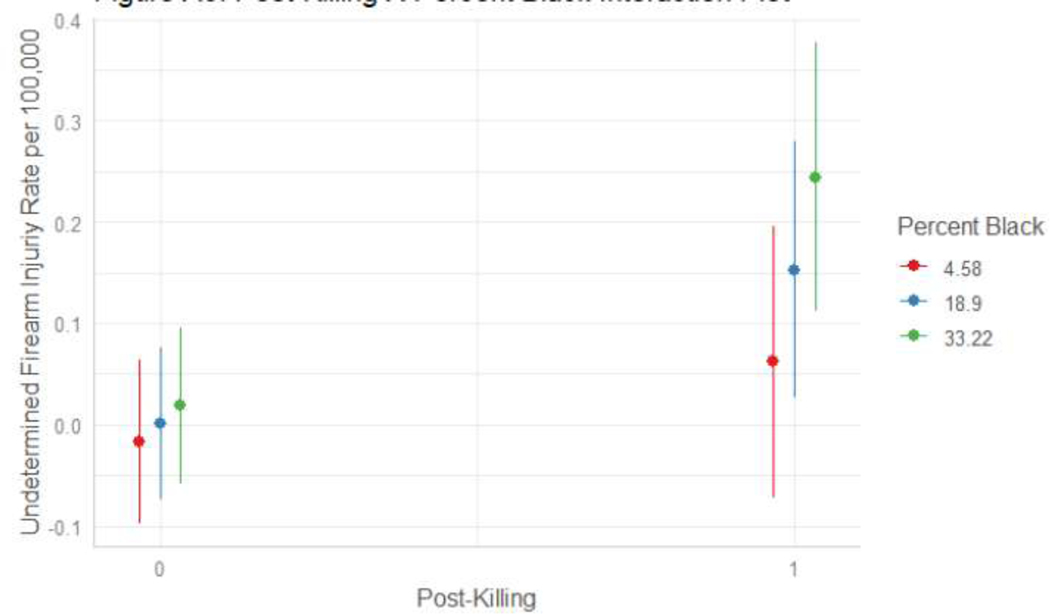
We leverage Minnesota Hospital Discharge data to create our dependent variable, firearm assault injuries per 100,000 residents. Inpatient and outpatient data from 2016–2020 utilizing International Classification of Diseases-10 codes X93-X95 were used to define firearm assault injuries. Recent studies of hospital administrative data suggest that firearm assaults are often misclassified as unintentional injuries or accidents when intent is unknown or ambiguous.¹⁸ We restrict our primary analyses to the patterns of known firearm assaults, but also provide an appendix providing identical analyses for the rate of unintentional firearm injuries added to the known assaults per 100,000 residents, as well as analyses for firearm injuries designated as “undetermined”. The spatiotemporal results we observe are robust to the choice of dependent measure. While our analysis focuses on the 2020 calendar year as 2021 injury data are not yet available, we also provide descriptive information in the appendix on the spatial and temporal pattern in Minneapolis homicides, as measured by the Minneapolis Police Department, to examine the robustness and persistence of patterns identified in the firearm injuries.

To measure the effects of the event of interest and to test the two major claims of the unrest, we create time indicators that measure the average rate in the period as compared to the pre-killing baseline, following previous empirical work on crime rates in Baltimore.¹⁵ The key exposure time indicators are a) the weekly linear time indicator, b) an event indicator for the police killing of George Floyd on 5/25/2020 (post-killing), and a linear week time counter post-killing. These are the focal time indicators of interest in the interrupted time series analysis, and represent the interrupted pattern and change in slope after the police killing of Mr. Floyd.

We also create event indicators at two other key points related to the COVID-19 pandemic: 3/13/2020 at the inception of Governor Walz’s State of Emergency order, and from 3/28–2020-5/28/2020 at the introduction and conclusion of this Stay-at-Home order.¹ These time indicators adjust for changes in firearm assault incidence related to significant policy events in the course of the COVID-19 pandemic and related patterns of social interaction. We also incorporate measures of police behavior from the Minneapolis Police Department. Specifically, we aggregate reported use of force incidents, police stops, and officer-involved shootings to both the week and ZCTA-week level from 2016–2020, placing each incident in each ZCTA-week by the date of incident and the longitude and latitude coordinates of the location of the event. We lag each measure of policing behavior to remove any simultaneity bias between policing and firearm assault incidence. These measures serve as our measures of policing activity in Minneapolis, and we adjust our event coefficients for any concurrent changes in police stops, uses of force, or shootings.

We also merge measures of seasonality onto the weekly hospital data. Following previous scholarship¹⁵ we include the weekly maximum temperature (degrees Fahrenheit), snowfall (in.), and precipitation (in.) from the Minnesota Department of Natural Resources as measured at the Minneapolis/St. Paul Threaded Record station. A measure of the average weekly number of hours of dark before 12pm is also included as further adjustment for seasonality. This measure is calculated via the ‘suncalc’ package in R¹⁹, which, conditional on the week and location, calculates the sunset on each particular day. We then calculate the time difference between sunset and midnight. We aggregate this to the average amount per day in each to represent our weekly measure of darkness before 12 midnight. Finally, we construct the proportion of days in the week K-12 Minneapolis Public Schools were in session based on school calendars from 2016–2020. These measures serve as essential seasonal controls that adjust the key time period estimates for expected seasonal changes in gun assault injury.

Spatial Zip Code Tabulation Area (ZCTA) simple feature boundary attributes, and each geography’s corresponding yearly American Community Survey (ACS) data, was accessed from The Census Bureau’s API using the ‘tidycensus’ package in R.²⁰ These data and boundary attributes can also be accessed through the IPUMS USA dataset.²¹ ZCTAs representing Minneapolis were determined by spatial intersection with the Minneapolis city boundary. Additionally, intersecting neighbors were defined as > 2 percent spatial overlap to identify ZCTAs that contain enough spatial overlap to have records in the Minneapolis Police Department data. We situate our panel at the ZCTA-level because the Minnesota Hospital Data’s lowest level of geography available is the ZCTA, and does not include more resolute information on the residences of those injured. We also acquire ZCTA-year data on percent Black and median household income from the American Community Survey 5-year estimates. Percent Black serves as our proxy for structural racism in our tests of spatial heterogeneity below, and we include median household income as a measure of socioeconomic status to control for the interrelationships between class and race. Table 1 below contains relays all variables included in the primary analyses and the sensitivity analyses in the appendix.

Table 1:

Variables and Data Sources in all Analyses

Variable	Data Source	Measurement
Firearm Assault Injury Rate	MHA Discharge Data	Injuries per 100,000
Firearm Assault+Unintentional Injury Rate*	MHA Discharge Data	Injuries per 100,000
Firearm Undetermined Injury Rate*	MHA Discharge Data	Injuries per 100,000
Murder Rate*	MPD Crime Data	Murders per 100,000
T		Linear Week Count
Post-Killing		0 pre-5/25/2020; 1 post-5/25/2020
T Post-Killing		Linear Week Count post-5/25/2020
COVID – State of Emergency	COVID-19 US Policy Database	0 pre-3/13/2020; 1 post-3/13/2020
COVID – Stay at Home	COVID-19 US Policy Database	0; 1 within 3/28-2020-5/28/2020
Mean Temperature Maximum	MNDNR Weather Data	Degrees Fahrenheit
Snowfall	MNDNR Weather Data	Inches
Precipitation	MNDNR Weather Data	Inches
Dark Before 12	Suncalc R Package	Hours of dark before midnight
Proportion of School Days	Minneapolis Public Schools	School days/7
Use of Forcet-1	MPD UOF Data	Lag rate per 1,000
Stopst-1	MPD Stops Data	Lag rate per 1,000
Officer Involved Shootingst-1	MPD OIS Data	Lag rate per 1,000
Median Household Income	ACS 5-Year Estimates	USD
Percent Black	ACS 5-Year Estimates	(Black Pop/Total Pop)*100

^*Denotes variable exclusively used in robustness checks in appendix

2.2. Statistical Method

Our analytical strategy is two-fold: we first estimate interrupted time-series models on week-level data, then estimate random-effects panel models with random ZCTA intercepts on Zip Code Tabulation Area (ZCTA)-week level data to corroborate and extend the aggregate findings incorporating both within- and between-ZCTA variation. Interrupted time series designs compare the levels of outcomes after a treatment or intervention to the mean outcome level in the pre-intervention period. The pre-treatment trend is assumed to serve as the counterfactual should treatment not have occurred (i.e. the trend in firearm injury incidence in the counterfactual scenario where the police killing of Mr. Floyd did not occur). The design exclusively uses within-unit over time variation, so time-stable confounders are uncorrelated with the time-varying treatment. However, the design is susceptible to time-varying confounders, which can vary alongside treatment timing, and we therefore include a suite of time-varying controls to strengthen our causal identification in the ITS design. Further, the design is susceptible to temporal autocorrelation in the series, and significant autocorrelation was detected at a lag of 1 in partial autocorrelation functions of the residuals, and therefore an AR(1) component was added to the overall time series model to account for this serial dependence. This effectively controls for the possibility of the focal event timing being confounded with recent changes in firearm injury incidence. We include a specification of the overall AR(1) time series model both with and without our indicators of police behavior, to examine whether the post-killing changes in firearm injury incidence are driven by changes in policing (i.e., the “depolicing” argument). Overall, the AR(1) interrupted time series models describe how firearm injury incidence changed on average across Minneapolis before and after the police killing of Mr. Floyd. Our full AR(1) specification is estimated via ordinary OLS in R and is formulated as follows:

$$y_t={\beta }_0+{\beta }_{1}Tim{e}_t+{\beta }_{2}PostKilling+{\beta }_{3}TimePos{t}_t+\varphi {\text{X}}_t+{\rho }_1{y}_{t-1}+{\in }_t$$

With ${\beta }_1$ the linear pre-killing trend, ${\text{β}}_2$ the discontinuity in the time series in the week of the police murder of Mr. Floyd, ${\beta }_3$ captures the linear time trend post-killing. ${\mathbf{X}}_{\mathbf{t}}$ are the time-varying controls (seasonality, police behavior, and COVID-19 policy indicators), and ${\text{ρ}}_1$ captures is the estimate of the AR(1) term.

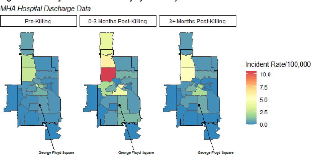
Subsequently, we estimate a random-effects model on ZCTA-week panel data to corroborate and extend the findings of the overall Minneapolis AR(1) interrupted time series models by using within ZCTA comparisons. The panel structure of the data allows us to examine the spatial heterogeneity of the police killing on firearm injury incidence across ZCTAs. In other words, these models allow for the examination of how the difference in firearm injury incidence pre-post was heterogeneous across space in Minneapolis. To test this hypothesis, we include a subsequent RE specification with a cross-level interaction between the post-killing indicator and percent Black to examine the spatial heterogeneity in the post-killing effect across communities and to assess the moderating influence of structural racism on the effect of the police killing (see also Figure 2).^22,23 Our base RE specification is estimated via restricted maximum likelihood in the ‘lme4’ package in the R statistical computing environment and is formulated as follows:

$$y_{ti}={\beta }_{0i}+{\beta }_{1}Tim{e}_t+{\beta }_{2}PostKillin{g}_t+{\beta }_{3}TimePos{t}_t+\varphi {\text{X}}_{ti}+{\in }_{ti}{\beta }_{0i}={\gamma }_{00}+u_{0i}$$

With ${\beta }_1$ the linear pre-killing trend, ${\text{β}}_2$ the discontinuity in the time series in the week of the police murder of Mr. Floyd, ${\beta }_3$ captures the linear time trend post-killing. ${\mathbf{X}}_{\mathbf{ti}}$ are the time-varying controls indexed by ZCTA (seasonality, police behavior, and COVID-19 policy indicators), and ${\beta }_{0i}$ represents the random intercept of each ZCTA. All data and code for data manipulation, merging, and analysis, apart from the restricted MHA data, are available in an online GitHub repository.

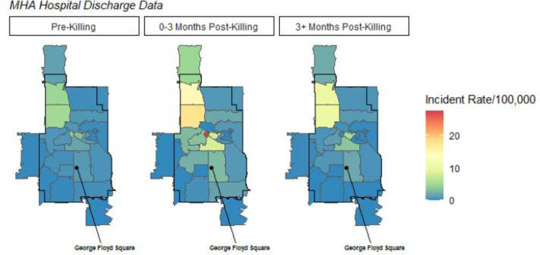
Figure 2:

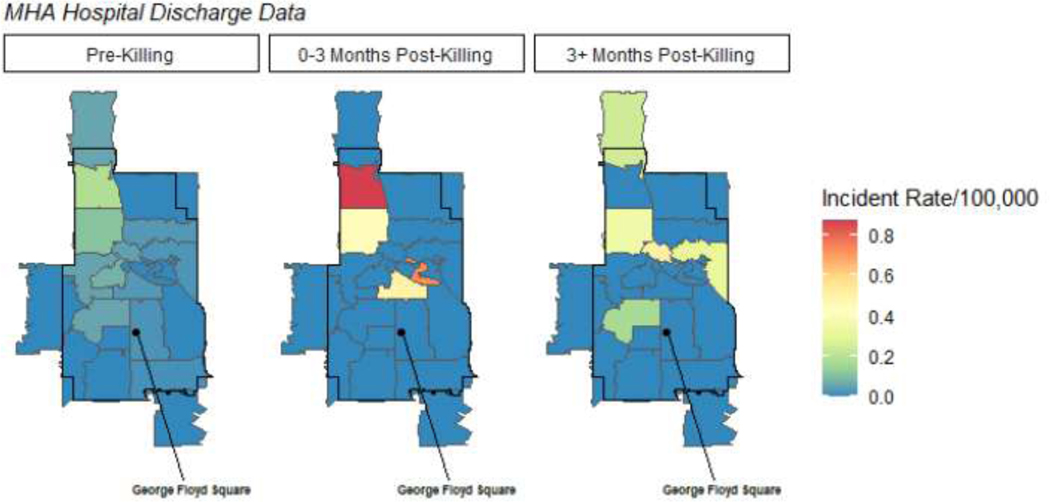
Weekly Firearm Assault Injury Rates by ZCTA and Period.

3. Results

3.1. Temporal Pattern of Firearm Assault Injuries

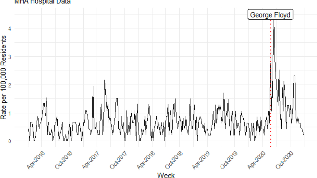
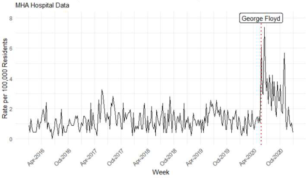
Figure 1 displays the weekly incidence of gun assault injuries from hospitals in Minneapolis from 2016–2020. We observe a sharp increase in the firearm assault injury rate from about .6 per 1,000 residents to a peak of 4.4 per 1,000 residents after the police killing of George Floyd, over a seven-fold increase. After an initial spike, the rate then fell to levels more consistent with the pre-killing period.

Figure 1:

Weekly Firearm Assault Injuries, 2016–2020

3.2. Spatiotemporal Pattern of Firearm Assault Injuries

After describing the temporal pattern in Figure 1, we next disaggregate the weekly data to local Zip Code Tabulation Areas (ZCTAs) to analyze the spatiotemporal variation in the rates of firearm assault. Figure 2 displays the firearm rates by Zip Code Tabulation Areas and period. In the Pre-Killing period (first panel of Figure 2), the ZCTAs do exhibit a spatial pattern, with the average ZCTA having a pre-killing firearm assault injury rate of .067 per 100,000, but with the rates ranging from 0 to 3.16 per 100,000. The temporal pattern apparent in Figure 1 emerges, but only for certain ZCTAs. Specifically, areas already marked by higher gun violence in the pre-treatment period experienced greater change across the time periods as compared to ZCTAs with very low firearm assault incidence. The area surrounding George Floyd Square experienced an increase in firearm assault injuries in the three months following Mr. Floyd’s death, but the red area representing the greatest spike is North Minneapolis, a historically Black community and a longstanding site of resistance to police violence and racial injustice. This includes the area of civil unrest on Plymouth Avenue in 1967, in which residents protested against maltreatment by police and local business owners.²⁴

3.3. Interrupted Time Series Models

Table 2 presents interrupted time series models of the firearm assault injury rate in Minneapolis from 2016–2020. Each model includes the interrupted time series time indicators, as well as controls for seasonality. Models 2, 3, and 5 introduce the measures of police behavior. The seasonality measures account for the expected seasonal change in gun assault injuries, and the measures of MPD police activity account for changes in police behavior in the post-killing periods and allow us to assess the extent to which “de-policing” accounted for the discontinuous change in firearm assault injury incidence. Models 3,4 and 5 are estimated on disaggregated weekly Zip Code Tabulation Area data, and include ZCTA random effects to account for the clustered data within ZCTAs across time. Controlling for seasonal expectations, Model 1 indicates that the rate of firearm assault injuries rose in the three months after the killing (labeled Post-Killing in the table), by an average of 1.78 firearm assault injuries per 100,000 residents. The post-killing linear trend indicates that the rate declined each week by.048 firearm assault injuries per 100,000, indicating that the rate did return to levels comparable to the pre-killing baseline after the initial spike by then end of 2020. Model 2 presents a specification introducing the measures of police behavior. The post-killing terms are stable when controlling for time-varying measures of police behavior, suggesting that the discontinuous change in firearm assault injury incidence cannot be attributed to changes in policing.

Table 2.

Interrupted Time Series Models of Firearm Assault Injuries

	Firearm Assault Injuries
	Rate per 100,000
	AR(1) TSR	AR(1) TSR	RE HLM	RE HLM	RE HLM +Int.
	(1)	(2)	(3)	(4)	(5)
T	0.001	−0.001	0.003	0.002	0.001
	(−0.0003|0.002)	(−0.003|0.001)	(0.0004|0.005)	(−0.0005|0.004)	(−0.002|0.004)
COVID - State of Emergency	−0.463	−0.411	−0.646	−0.506	−0.439
	(−1.026|0.100)	(−0.995|0.173)	(−2.001|0.708)	(−1.864|0.853)	(−1.917|1.040)
COVID - Stay at Home	0.403	0.416	0.242	0.156	0.189
	(−0.179|0.984)	(−0.183|1.016)	(−1.151|1.636)	(−1.240|1.553)	(−1.331|1.709)
Post-Killing	1.781	1.775	1.330	1.277	0.282
	(1.176|2.387)	(1.137|2.414)	(−0.092|2.751)	(−0.149|2.703)	(−1.375|1.938)
T Post-Killing	−0.048	−0.047	−0.035	−0.032	−0.036
	(−0.068|−0.028)	(−0.070|−0.025)	(−0.081|0.011)	(−0.078|0.015)	(−0.086|0.015)
MPD Use of Force t-1		−0.015		−0.130	−0.123
		(−1.400|1.370)		(−0.184|−0.077)	(−0.175|−0.070)
MPD Stops t-1		−0.121		0.035	0.076
		(−0.365|0.122)		(0.019|0.051)	(0.055|0.098)
MPD OIS t-1		−27.382		−1.953	−1.668
		(−67.727|12.964)		(−12.946|9.040)	(−13.095|9.759)
AR(1)	0.142	0.065
	(0.021|0.263)	(−0.071|0.201)
Median HH Income					0.00001
					(−0.00001|0.00002)
Percent Black					0.038
					(0.014|0.062)
Post-Killing X Percent Black					0.063
					(0.032|0.094)
Constant	0.579	0.931	0.800	0.834	−0.412
	(−0.194|1.352)	(−0.204|2.066)	(−1.093|2.694)	(−1.073|2.740)	(−2.785|1.961)
SD(ZCTA)			0.904	0.922	0.504
SD(Residual)			5.352	5.364	5.577
Observations	260	217	5,993	5,928	5,460
R2	0.385	0.407
Log Likelihood			−18,592.500	−18,406.520	−17,172.070
Akaike Inf. Crit.			37,210.990	36,845.050	34,382.150
Bayesian Inf. Crit.			37,298.070	36,952.040	34,507.650
Residual Std. Error	0.463 (df = 248)	0.474 (df = 202)
F Statistic	14.117*** (df = 11; 248)	9.898*** (df = 14; 202)
Models include controls for seasonality.	95% Confidence Intervals in parentheses

In Models 3 and 4 these results are corroborated using the ZCTA-week panel data, showing a 1.33 increase in firearm assault injury incidents per 100,000 residents in the immediate post-killing period, followed by a weekly decline (−.035) in the post-killing period. After controlling for changes in police behavior in the panel model (Model 4), the event time indicators remain largely unaltered in direction or magnitude, suggesting that ZCTA-level changes in local policing did little to drive the increase in gun violence. If changes in police behavior had been a primary driver of this post-killing increase, then the inclusion of police measures should have significantly attenuated the post-killing effect, which we do not observe across any specifications at the city- or ZCTA-levels. Additionally, the post-killing effects remain after controlling for state policy in relation to the COVID-19 pandemic, suggesting that the increase in gun violence is not entirely due to pandemic-related policy changes, and the resulting changes in behavior and movement, This analysis provides evidence of a “Minneapolis effect,” as the firearm assault injury rate increased above and beyond seasonal expectations, but this rise was not driven by changes in police behavior or by COVID-19-related state policy changes. Importantly, the size of the weekly firearm assault rate decreases in the post-killing period suggest that firearm injury rates rate did, on average, return to pre-killing levels at least as of the end of 2020.

3.4. Spatial Heterogeneity in Post-Killing Effects

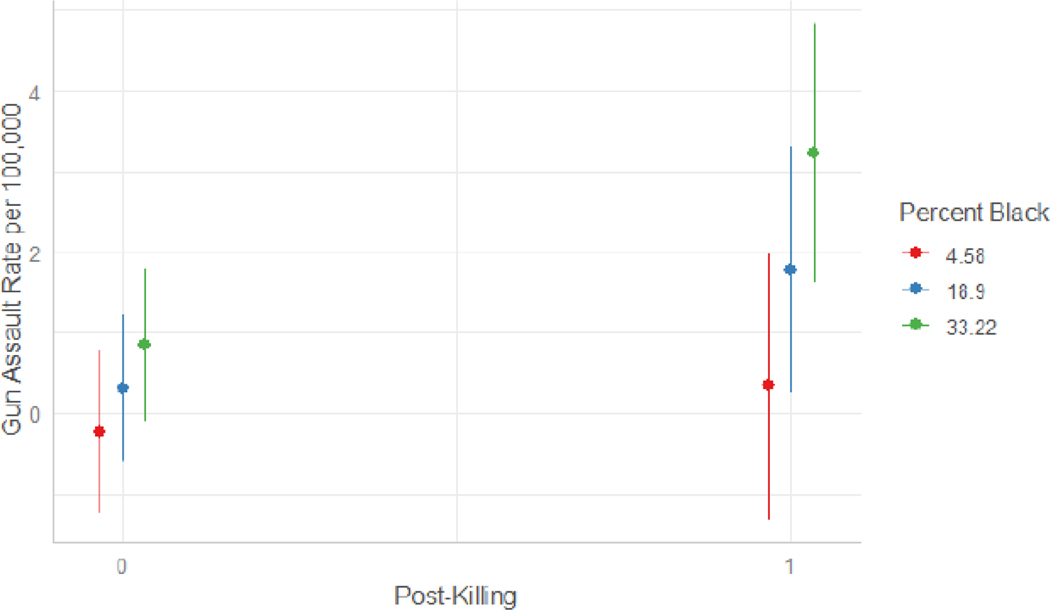
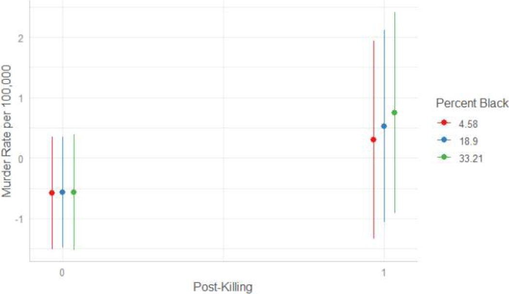
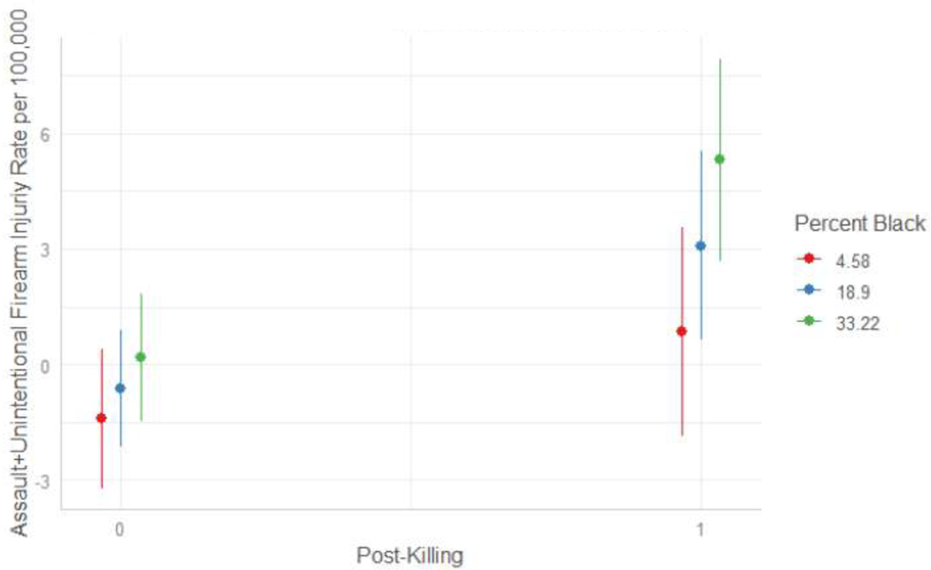
Model 5 in Table 2 relays the results of a random effects model that includes a cross-level interaction between the post-killing time indicator and ZCTA percent Black, which allows the post-killing effect to vary conditional upon the percent Black in a given ZCTA. The statistically significant interaction effect suggests that the post-killing increase was greater in places with higher percent Black, as the interaction term indicates that a one percent increase in percent Black increased the post-killing effect by about .063 firearm assault incidents per 100,000 residents. The main effect of percent Black captures the spatial heterogeneity in firearm assault injury incidence by percent Black in the pre-killing period. This term is statistically significant and positive, indicative of higher levels of violence in Black neighborhoods in the pre-killing period, consistent with the spatial heterogeneity depicted in Figure 2. This highlights how the neighborhoods already experiencing higher levels of gun assault injury incidence were also those that experienced the greatest brunt of the increase in Minneapolis post-killing. Further, the main effect for post-killing is statistically nonsignificant, and is reduced in magnitude, suggesting ZCTAs with no or very few Black residents did not experience a significant increase in gun assault injury incidence. Figure 3 plots the interaction effect from Model 5, showing that ZCTAs characterized by one standard deviation above the average in percent Black experienced far greater post-killing increases as compared to ZCTAs at below average levels of Black residents. These spatiotemporal patterns indicate the heterogeneous spatial effects of the police killing of George Floyd, as not all spaces in Minneapolis experienced the magnitude of post-killing increase, or any increase at all, as economically disadvantaged, Black neighborhoods did.

Figure 3:

Post-Killing X Percent Black Interaction Plot

4. Discussion

We find that firearm assault injury rates spiked dramatically and then declined in Minneapolis after the murder of George Floyd by police, even in models that adjust for seasonality, changes in police behavior, and COVID-19-related state policy changes. Further, our models indicate that changes in police behavior did not drive the temporal changes in gun assault injuries, which suggest that “de-policing,” to the extent it occurred post-killing, did not play a primary role in driving gun violence upwards. Similar patterns are also evident for firearm injuries classified as assault or “unintentional”, as well as “undetermined” (See Appendix). These findings reveal a “Minneapolis effect,” wherein an extreme and high-profile police killing significantly altered the temporal pattern of firearm assault injuries. This finding is also consistent with past studies of cities such as Baltimore after the Freddie Gray police killing.¹⁵ The present study, however, adds important information to this literature by considering a measure of gun violence that is less prone to bias or selection concerns, as well as establishing the spatial heterogeneity in these deleterious effects on firearm violence.

Our study, however, is not without its limitations. First, we caution that our data and analysis are limited to a single jurisdiction in a period of large-scale social change in response to COVID-19, economic recession, and social unrest. Second, our interrupted time series design relies upon the assumption that the change in firearm incidence in the week of the police killing is unrelated to unmeasured time-varying characteristics. If other unmeasured contemporaneous changes also drove the increase in firearm injury, the validity of our estimates would be threatened. Finally, we explore only one mechanism of effect heterogeneity, percent Black, and the impacts of police violence on communities could perhaps vary amongst other social or economic dimensions. Although a full exploration of the mechanisms for this increase is beyond the scope of our analysis, the localized and racialized patterns we observe are consistent with accounts based on structural racism, legal estrangement and legal cynicism. Further research is clearly needed to elucidate these processes, but the pattern of findings is consistent with the idea that police violence impacts vulnerable communities by destabilizing social order and threatening public safety.

5. Public Health Implications

Both firearm injuries and police violence are urgent public health emergencies. Our findings here highlight severe public health consequences of police violence that extend beyond individual incidents of police brutality.^24,25 Further, we find that communities already experiencing higher levels of social disadvantage and firearm assault incidence had disproportionate increases in firearm assault injury after the murder of Mr. Floyd, suggesting that police violence can exacerbate already existing social inequalities in firearm injury. In fact, the neighborhoods that suffered the greatest increases in 2020 were precisely the sites of previous police maltreatment and uprisings against police violence in the 1960s.²⁶ These findings speak to the traumatizing effects of police violence and the short- and long-term public health consequences for communities, particularly Black communities.^1,2

Appendix

Homicide Data and the Robustness and Persistence of Results

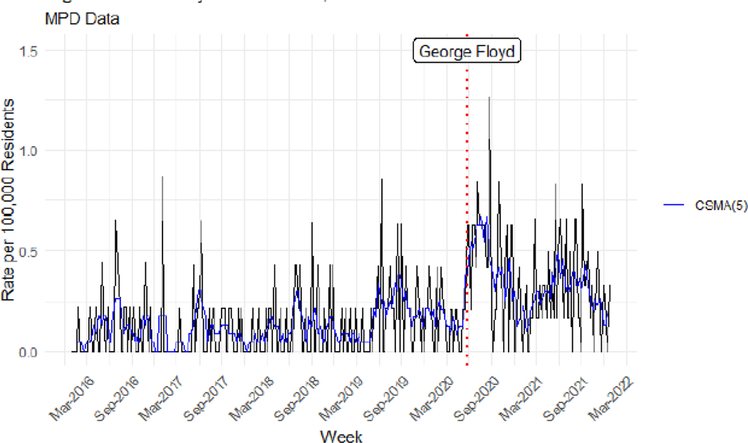
Our analysis focuses on the 2020 calendar year when complete hospital data and information on key covariates are available. Although 2021 injury data are not yet available, we can provide descriptive information on the spatial and temporal pattern in Minneapolis homicides to examine the robustness and persistence of patterns identified above. Figure A1 displays the weekly murder rate using Minneapolis Police Department data from 2016–2021. A 5-week centered simple moving average (assuming equal weights across the window) is plotted on top of the weekly murder rates in Minneapolis to smooth out the variability present in the week-to-week murder rates. Although murder rates are much lower than gun assault rates (as gun murders represent a small part of overall gun assaults), the post-killing spike observed in the hospital data is also present in the murder data, with a jump from an average of roughly .012 murders per 100,000 residents to 1.26 murders per 100,000 at its weekly peak, a ten-fold increase. Incorporating data from 2021 further contextualizes the potential longer-term impact of the murder of Mr. Floyd and the longer-term impact of exposure to incidents of police violence. Weekly murder rates did not return to their pre-killing levels in 2021, maintaining a mean weekly murder rate per 100,000 residents of about .034. This weekly rate is significantly higher than the pre-killing mean of .012 (Welch’s t(60.3) = −7.05, p <.001).

Figure A1:

Weekly Murder Rate,2016–2021

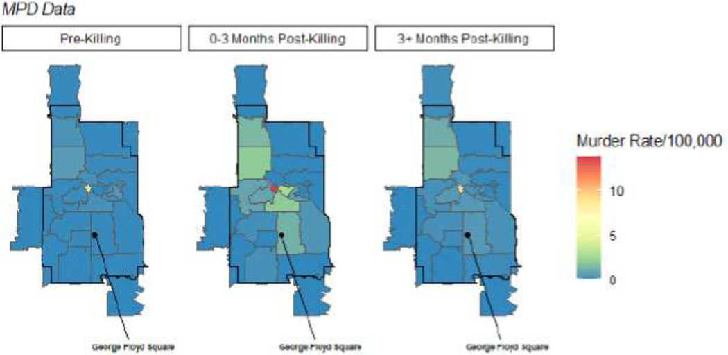
Figure A2 similarly contextualizes the spatial findings using geolocated Minneapolis Police Department murders into 2021. The spatial location of each MPD murder event is the incident ZCTA, rather than the patient’s residence ZCTA in the hospital administrative data, so the spatial rates here are not directly analogous to those in Figure 2 in the main text. This is apparent in the spatially small ZCTA 55402, representing downtown Minneapolis. The number of murders is high due to the confluence of people downtown, but the ZCTA has a relatively small residential denominator. This is in contrast to the gun assault rates in 55402, which measures the gun assault incidence for residents of 55402, as opposed to overall incidence in the ZCTA. Although the weekly murder rates are lower than that of the gun assault incidence, we observe a similar spatial pattern in post-killing increases in murders. Further, while we also see a similar decline in the 3+ months post-killing period from the initial three months post-killing with the inclusion of 2021 into this period, the weekly murder rates do not return to pre-killing levels for certain ZCTAs, indicating that, for some communities, the elevated rates of violence persisted into 2021.

Figure A2:

Weekly Murder Rates by ZCTA and priod

The spatiotemporal visualizations above are corroborated by interrupted time series models at both the city-week and ZCTA-week levels. Similar to Table 2 in the main text, a significant increase in murders was observed, followed by modest linear decreases in the post-killing period across all specifications. However, the interaction term in Model 5, albeit similar in direction to that of Table 2 Model 5, is less strong, suggesting perhaps that the spatial heterogeneity in the post-killing effect was moderated by a factor other than racial demographic composition. However, we caution against overinterpreting this effect, as downtown ZCTAs (e.g., 55402) had a higher increase in murders, but these often involve non-residents in these ZCTAs. Such ZCTAs have a relatively advantaged residential population but experienced a larger discontinuity in murder rate, and could be suppressing the broader spatial pattern.

Table A1.

Interrupted Time Series Models of the Murder Rate

	Murder Rate
	Rate per 100,000
	AR(1) TSR	AR(1) TSR	RE HLM	RE HLM	RE HLM +Int.
	(1)	(2)	(3)	(4)	(5)
T	0.001	0.001	0.0001	0.0001	0.0001
	(0.0002|0.001)	(−0.0002|0.001)	(0.00002|0.0002)	(−0.00001|0.0002)	(−0.00002|0.0002)
COVID - State of Emergency	−0.025	−0.044	−0.428	−0.332	−0.264
	(−0.255|0.205)	(−0.282|0.194)	(−1.881|1.025)	(−1.785|1.121)	(−1.812|1.283)
COVID - Stay at Home	−0.038	−0.028	−0.262	−0.331	−0.333
	(−0.275|0.199)	(−0.272|0.217)	(−1.756|1.231)	(−1.823|1.162)	(−1.924|1.257)
Post-Killing	0.309	0.283	0.887	0.848	0.809
	(0.078|0.541)	(0.042|0.525)	(−0.639|2.413)	(−0.677|2.373)	(−0.928|2.546)
T Post-Killing	−0.004	−0.004	−0.033	−0.032	−0.040
	(−0.006|−0.002)	(−0.006|−0.002)	(−0.085|0.019)	(−0.084|0.020)	(−0.095|0.016)
MPD Use of Force t-1		0.159		−0.095	−0.036
		(−0.346|0.664)		(−0.150|−0.039)	(−0.088|0.015)
MPD Stops t-1		−0.054		0.020	0.074
		(−0.148|0.039)		(0.003|0.037)	(0.055|0.092)
MPD OIS t-1		5.056		2.313	2.586
		(−11.273|21.38 5)		(−9.418|14.045)	(−9.350|14.521)
AR(1)	−0.107	−0.139
	(−0.220|0.006)	(−0.261|−0.016)
Median HH Income					−0.00000
					(−0.00001|0.00001)
Percent Black					0.0005
					(−0.014|0.015)
Post-Killing X Percent Black					0.015
					(−0.017|0.048)
Constant	−0.028	0.038	0.237	0.306	0.461
	(−0.303|0.247)	(−0.354|0.429)	(−1.845|2.319)	(−1.779|2.392)	(−1.819|2.741)
SD(ZCTA)			0.904	0.922	0.504
SD(Residual)			5.352	5.364	5.577
Observations	312	269	5,929	5,926	5,458
R2	0.297	0.315
Log Likelihood			−18,795.350	−18,783.110	−17,400.650
Akaike Inf. Crit.			37,616.700	37,598.210	34,839.310
Bayesian Inf. Crit.			37,703.640	37,705.210	34,964.800
Residual Std. Error	0.192 (df = 300)	0.197 (df = 254)
F Statistic	11.538*** (df = 11; 300)	8.334*** (df = 14; 254)
Models include controls for seasonality.	95% Confidence Intervals in parentheses

Figure A3:

Post-Killing X Percent Black Interaction Plot.

Unintentional Firearm Injury Analyses

Figure A4:

Weekly Firearm Assault + Unintentional Injuries, 2016–2020

Figure A5:

Weekly Firearm Assault + Unintentional Injuries Rates by ZCTA and Period

Table A2.

Interrupted Time Series Models of Firearm Assault+Unintentional Injuries

	Firearm Assault+Unintentional Injuries
	Rate per 100,000
	AR(1) TSR	AR(1) TSR	RE HLM	RE HLM	RE HLM +Int.
	(1)	(2)	(3)	(4)	(5)
T	0.002	−0.002	0.005	0.004	0.003
	(0.0001|0.003)	(−0.005|0.001)	(0.001|0.009)	(0.0001|0.008)	(−0.001|0.008)
COVID - State of Emergency	−0.608	−0.464	−0.178	−0.022	0.039
	(−1.486|0.270)	(−1.380|0.452)	(−2.343|1.987)	(−2.190|2.146)	(−2.269|2.347)
COVID - Stay at Home	0.445	0.451	−0.726	−0.844	−0.877
	(−0.464|1.354)	(−0.490|1.393)	(−2.962|1.509)	(−3.080|1.392)	(−3.249|1.496)
Post-Killing	3.394	3.341	3.606	3.493	1.812
	(2.443|4.345)	(2.337|4.344)	(1.323|5.890)	(1.208|5.778)	(−0.774|4.397)
T Post-Killing	−0.097	−0.092	−0.160	−0.156	−0.163
	(−0.128|−0.065)	(−0.127|−0.057)	(−0.235|−0.085)	(−0.232|−0.081)	(−0.242|−0.084)
MPD Use of Force t-1		−0.083		−0.186	−0.169
		(−2.252|2.086)		(−0.272|−0.100)	(−0.255|−0.082)
MPD Stops t-1		−0.265		0.022	0.042
		(−0.649|0.118)		(−0.011|0.054)	(0.005|0.079)
MPD OIS t-1		−10.263		−3.256	−2.942
		(−73.259|52.733)		(−20.666|14.155)	(−20.784|14.900)
AR(1)	0.045	−0.038
	(−0.075|0.165)	(−0.173|0.096)
Median HH Income					0.00000
					(−0.00003|0.00004)
Percent Black					0.055
					(−0.003|0.113)
Post-Killing X Percent Black					0.100
					(0.052|0.148)
Constant	0.411	1.290	−0.280	−0.236	−1.599
	(−0.787|1.609)	(−0.483|3.063)	(−3.369|2.809)	(−3.340|2.868)	(−5.960|2.762)
SD(ZCTA)			1.779	1.916	1.449
SD(Residual)			8.493	8.494	8.704
Observations	260	217	5,770	5,748	5,460
R2	0.491	0.513
Log Likelihood			−20,564.490	−20,488.920	−19,603.880
Akaike Inf. Crit.			41,154.970	41,009.850	39,245.770
Bayesian Inf. Crit.			41,241.560	41,116.350	39,371.270
Residual Std. Error	0.721 (df = 248)	0.742 (df = 202)
F Statistic	21.786*** (df = 11; 248)	15.216*** (df = 14; 202)
Models include controls for seasonality.	95% Confidence Intervals in parentheses

Figure A6:

Post-Killing X Percent Black Interaction Plot

Undetermined Firearm Injuries Analyses

Figure A7:

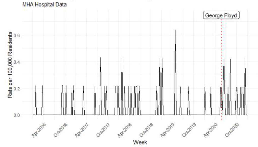
Weekly Firearm Undetermined Injuries, 2016–2020

Figure A8:

Weekly Firearm Undetermined Injury Rates by ZCTA and Period

Table A3.

Interrupted Time Series Models of Firearm Undetermined Injuries

	Firearm Undetermined Injuries
	Rate per 100,000
	AR(1) TSR	AR(1) TSR	RE HLM	RE HLM	RE HLM +Int.
	(1)	(2)	(3)	(4)	(5)
T	0.00002	−0.0001	0.00000	−0.00001	0.00001
	(−0.0002|0.0002)	(−0.001|0.0003)	(−0.0002|0.0002)	(−0.0002|0.0002)	(−0.0002|0.0002)
COVID - State of Emergency	−0.065	−0.065	−0.049	−0.048	−0.052
	(−0.192|0.062)	(−0.200|0.071)	(−0.161|0.063)	(−0.161|0.065)	(−0.175|0.070)
COVID - Stay at Home	0.050	0.054	0.039	0.039	0.042
	(−0.080|0.181)	(−0.084|0.193)	(−0.076|0.154)	(−0.077|0.154)	(−0.084|0.168)
Post-Killing	0.164	0.170	0.138	0.138	0.054
	(0.029|0.299)	(0.023|0.316)	(0.020|0.255)	(0.020|0.257)	(−0.083|0.192)
T Post-Killing	−0.002	−0.002	−0.002	−0.002	−0.002
	(−0.006|0.002)	(−0.007|0.003)	(−0.006|0.002)	(−0.006|0.002)	(−0.006|0.002)
MPD Use of Force t-1		0.099		−0.0004	−0.0005
		(−0.221|0.420)		(−0.005|0.004)	(−0.005|0.004)
MPD Stops t-1		−0.007		−0.0001	−0.0002
		(−0.064|0.049)		(−0.001|0.001)	(−0.002|0.001)
MPD OIS t-1		−3.299		−0.160	−0.143
		(−12.654|6.055)		(−1.071|0.751)	(−1.090|0.805)
AR(1)	−0.058	−0.085
	(−0.183|0.067)	(−0.224|0.053)
Median HH Income					−0.00000
					(−0.00000|0.00000)
Percent Black					0.001
					(−0.001|0.003)
Post-Killing X Percent Black					0.005
					(0.003|0.008)
Constant	0.075	0.194	0.009	0.010	0.008
	(−0.098|0.249)	(−0.071|0.459)	(−0.146|0.163)	(−0.146|0.166)	(−0.185|0.201)
SD(ZCTA)			0.046	0.046	0.037
SD(Residual)			0.442	0.444	0.462
Observations	260	217	5,993	5,928	5,460
R2	0.057	0.068
Log Likelihood			−3,664.154	−3,668.384	−3,618.112
Akaike Inf. Crit.			7,354.308	7,368.768	7,274.223
Bayesian Inf. Crit.			7,441.387	7,475.767	7,399.722
Residual Std. Error	0.104 (df = 248)	0.110 (df = 202)
F Statistic	1.373 (df = 11; 248)	1.051 (df = 14; 202)
Models include controls for seasonality.	95% Confidence Intervals in parentheses

Figure A9:

Post-Killing X Percent Black Interaction Plot

Table A4.

Interrupted Time Series Models of Firearm Assault Injuries

	Firearm Assault Injuries
	Rate per 100,000
	AR(1) TSR	AR(1) TSR	RE HLM	RE HLM	RE HLM +Int.
	(1)	(2)	(3)	(4)	(5)
T	0.001	−0.001	0.003	0.002	0.001
	(−0.0001|0.002)	(−0.003|0.001)	(0.0004|0.005)	(−0.0004|0.004)	(−0.002|0.004)
COVID - State of Emergency	−0.148	−0.063	−0.520	−0.352	−0.313
	(−0.786|0.490)	(−0.706|0.580)	(−2.114|1.074)	(−1.951|1.246)	(−2.052|1.427)
COVID - Stay at Home	−0.016	−0.032	0.081	−0.037	0.028
	(−0.712|0.681)	(−0.732|0.669)	(−1.659|1.821)	(−1.781|1.707)	(−1.869|1.926)
Post-Killing	2.545	2.556	1.611	1.617	0.563
	(1.614|3.477)	(1.619|3.493)	(−0.716|3.938)	(−0.715|3.950)	(−2.040|3.166)
1 Month Post	−0.699	−0.853	−0.013	−0.067	0.052
	(−1.906|0.509)	(−2.080|0.374)	(−3.029|3.003)	(−3.090|2.956)	(−3.237|3.342)
2 Months Post	−1.241	−1.538	−0.902	−1.059	−0.972
	(−2.454|−0.028)	(−2.785|−0.292)	(−3.931|2.127)	(−4.096|1.977)	(−4.276|2.331)
3 Months Post	−2.128	−2.355	−1.248	−1.331	−1.337
	(−3.345|-0.911)	(−3.596|-1.114)	(−4.288|1.791)	(−4.377|1.716)	(−4.652|1.977)
4 Months Post	−1.871	−2.021	−1.176	−1.145	−1.156
	(−3.085|−0.656)	(−3.252|−0.790)	(−4.210|1.858)	(−4.185|1.896)	(−4.464|2.153)
5 Months Post	−2.121	−2.111	−1.372	−1.353	−1.401
	(−3.334|−0.907)	(−3.339|−0.884)	(−4.402|1.658)	(−4.390|1.684)	(−4.706|1.903)
6 Months Post	−1.330	−1.337	−0.249	−0.304	−0.179
	(−2.548|−0.111)	(−2.566|−0.108)	(−3.292|2.794)	(−3.355|2.746)	(−3.498|3.140)
7+ Months Post	−2.489	−2.485	−1.527	−1.524	−1.566
	(−3.672|−1.307)	(−3.674|−1.295)	(−4.480|1.426)	(−4.484|1.435)	(−4.786|1.654)
MPD Use of Force t-1		−0.732		−0.130	−0.123
		(−2.145|0.680)		(−0.184|−0.077)	(−0.175|−0.070)
MPD Stops t-1		−0.182		0.035	0.077
		(−0.415|0.050)		(0.019|0.051)	(0.055|0.098)
MPD OIS t-1		−30.131		−2.053	−1.773
		(−68.210|7.948)		(−13.048|8.942)	(−13.202|9.657)
AR(1)					0.00001
					(−0.00001|0.00002)
Median HH Income					0.038
					(0.014|0.062)
Percent Black					0.063
					(0.032|0.094)
Post-Killing X Percent Black	0.722	1.263	0.878	0.924	−0.320
	(−0.029|1.474)	(0.178|2.348)	(−1.039|2.794)	(−1.006|2.854)	(−2.715|2.076)
SD(ZCTA)			0.817	0.922	0.504
SD(Residual)			5.353	5.364	5.578
Observations	261	217	5,993	5,928	5,460
R2	0.436	0.485
Log Likelihood			−18,582.870	−18,396.930	−17,161.870
Akaike Inf. Crit.			37,203.730	36,837.860	34,373.740
Bayesian Inf. Crit.			37,331.000	36,984.990	34,538.870
Residual Std. Error	0.447 (df = 244)	0.448 (df = 197)
F Statistic	11.808*** (df = 16; 244)	9.761*** (df = 19; 197)
Models include controls for seasonality.	95% Confidence Intervals in parentheses

References and Notes

- 1.Exclusion Muller C. and exploitation: The incarceration of black Americans from slavery to the present.” Science. 2017;374(6565):282–286. [DOI] [PubMed] [Google Scholar]
- 2.Page J, & Soss J. The predatory dimensions of criminal justice.” Science. 2021;374(6565): 291–294. [DOI] [PubMed] [Google Scholar]
- 3.Nummi J, Jennings C, Feagin J. #BlackLivesMatter: Innovative black resistance. Sociological Forum. 2019;34:1042–1064. [Google Scholar]
- 4.Edwards F, Lee H, Esposito M. Risk of being killed by police use of force in the United States by age, race–ethnicity, and sex. Proceedings of the National Academy of Sciences. 2019;116 (34):16793–16798. [DOI] [PMC free article] [PubMed] [Google Scholar]
- 5.Wrigley-Field E, Garcia S, Leider JP, Robertson C, Wurtz R. Racial disparities in COVID-19 and excess mortality in Minnesota. Socius. 2020; 6: 2378023120980918. [DOI] [PMC free article] [PubMed] [Google Scholar]
- 6.Jany L, Sawyer L. Gun violence soars amid crises of health, public trust, officer reluctance.” Star Tribune. June 2020. https://www.startribune.com/surge-in-gun-violence-tests-minneapolis-leaders/571524202/
- 7.Shjarback JA, Pyrooz DC, Wolfe SE, Decker SH. De-policing and crime in the wake of Ferguson: Racialized changes in the quantity and quality of policing among Missouri police departments. Journal of Criminal Justice 2017;50:42–52. [Google Scholar]
- 8.Federal Bureau of Investigation. FBI releases 2020 crime statistics. September 29th, 2021. https://www.fbi.gov/news/pressrel/press-releases/fbi-releases-2020-crime-statistics [Google Scholar]
- 9.Ssentongo P, Fronterre C, Ssentongo AE, et al. Gun violence incidence during the COVID-19 pandemic is higher than before the pandemic in the United States. Scientific Reports. 2021; 11:20654. [DOI] [PMC free article] [PubMed] [Google Scholar]
- 10.Nagin DS. Deterrence: A review of the evidence by a criminologist for economists. Annual Review of Economics. 2013;5(1):83–105. [Google Scholar]
- 11.Bell MC. Police reform and the dismantling of legal estrangement. The Yale Law Journal. 2017: 2054–2150.
- 12.Black D. Violent structures. In Zahn MA, Brownstein HH, Jackson SI. Violence: From theory to research. 1st Edition. Routledge; 2004:153–166. [Google Scholar]
- 13.Ferguson Rosenfeld R. and police use of deadly force. Missouri Law Review. 2015;80:1077. [Google Scholar]
- 14.Pyrooz DC, Decker SH, Wolfe SE, Shjarback JA. Was there a Ferguson effect on crime rates in large US cities?. Journal of Criminal Justice. 2016:46;1–8. [Google Scholar]
- 15.Morgan SL, & Pally J. Ferguson, Gray, and Davis: An analysis of recorded crime incidents and arrests in Baltimore City, March 2010 through December 2015. socArxiv. Preprint posted online February 11th, 2020. https://osf.io/preprints/socarxiv/nshme/
- 16.Wu DT, Moore JC, Bowen DA, et al. Proportion of violent injuries unreported to law enforcement.” JAMA Internal Medicine 2019;179(1): 111–112. [DOI] [PMC free article] [PubMed] [Google Scholar]
- 17.Desmond M, Papachristos AV, Kirk DS. Police violence and citizen crime reporting in the black community. American Sociological Review 2016;81(5):857–876. [Google Scholar]
- 18.Barber C, Goralnick E, Miller M. The problem with ICD-coded firearm injuries. JAMA Internal Medicine. 2021;181(8):1132–1133. [DOI] [PubMed] [Google Scholar]
- 19.Thieurmel B. and Elmarhraoui A. suncalc: Compute Sun Position, Sunlight Phases, Moon Position and Lunar Phase. 2019;R package version 0.5. https://CRAN.Rproject.org/package=suncalc
- 20.Walker K, Herman M. tidycensus: Load US census boundary and attribute data as ‘tidyverse’ and ‘sf’-ready data frames.” 2021;R package version 1.1. https://CRAN.Rproject.org/package=tidycensus
- 21.Ruggles S, Flood S, Foster S, et al. IPUMS USA: Version 11.0. 2021: Minneapolis, MN: IPUMS. 10.18128/D010.V11.0. [DOI] [Google Scholar]
- 22.Bates D, Machler M, Bolker B, and Walker S. Fitting linear mixed-effects models using lme4. Journal of Statistical Software. 2015;67(1): 1–48. [Google Scholar]
- 23.Kuznetsova A, Brockhoff PB, Christensen RHB. lmerTest package: Tests in linear mixed effects models. Journal of Statistical Software. 2017;82(13):1–26. [Google Scholar]
- 24.American Public Health Association. Addressing law enforcement violence as a public health issue. Policy no. 201811, November 13, 2018. Available at: https://www.apha.org/Policies-and-Advocacy/Public-Health-Policy-Statements/PolicyDatabase/2019/01/29/Law-Enforcement-Violence. Accessed July 13, 2022. [Google Scholar]
- 25.American Public Health Association. Structural racism is a public health crisis: Impact on the black community. Policy no. LB20–04, October 24, 2020. Available at: https://www.apha.org/policies-and-advocacy/public-health-policy-statements/policydatabase/2021/01/13/structural-racism-is-a-public-health-crisis. Accessed July 13, 2022. [Google Scholar]
- 26.Marks S. Civil unrest on Plymouth Avenue, Minneapolis, 1967. MNopedia, https://www.mnopedia.org/event/civil-unrest-plymouth-avenue-minneapolis-1967. Published December 21st, 2015. Updated July 15, 2021. Accessed july 7th, 2022.