Unsupervised deep network for image texture transformation: Improving the quality of cross-correlation analysis and mechanical vortex visualisation during cardiac fibrillation

Abstract

Visualisation of cardiac fibrillation plays a very considerable role in cardiophysiological study and clinical applications. One of the ways to obtain the image of these phenomena is the registration of mechanical displacement fields reflecting the track from electrical activity. In this work, we read these fields using cross-correlation analysis from the video of open pig's epicardium at the start of fibrillation recorded with electrocardiogram. However, the quality of obtained displacement fields remains low due to the weak pixels heterogeneity of the frames. It disables to see more clearly such interesting phenomena as mechanical vortexes that underline the mechanical dysfunction of fibrillation. The applying of chemical or mechanical markers to solve this problem can affect the course of natural processes and falsify the results. Therefore, we developed a novel scheme of an unsupervised deep neural network that is based on the state-of-art positional coding technology for a multilayer perceptron. This network enables to generate a couple of frames with a more heterogeneous pixel texture, that is more suitable for cross-correlation analysis methods, from two consecutive frames. The novel network scheme was tested on synthetic pairs of images with different texture heterogeneity and frequency of displacement fields and also it was compared with different filters on our cardiac tissue image dataset. The testing showed that the displacement fields obtained with our method are closer to the ground truth than those which were computed only with the cross-correlation analysis in low contrast images case where filtering is impossible. Moreover, our model showed the best results comparing with the one of the popular filter CLAHE on our dataset. As a result, using our approach, it was possible to register more clearly a mechanical vortex on the epicardium at the start of fibrillation continuously for several milliseconds for the first time.

1. Introduction

Today, the cross-correlation methods are widely used in many scientific areas. Particle Image Velocimetry (PIV) [1] and Digital Image Correlation (DIC) [2] are turned out to be the most spread instruments for applying in different tasks. They have undergone a long evolution and have become one of the most reliable methods for obtaining displacement and deformation fields from video recordings of fluids and various object surfaces. Thus, DIC and PIV were applied in biological applications for search of biomechanics [3],[4],[5],[6],[7]. However, important to note that the quality of information depends on particle or speckle intensity, their shape and also on the pixel heterogeneity of the image [8],[9],[10],[11]. Thus, experimenters strive to create the appropriate conditions, in addition, to applying post-processing (filtering) to obtain the suitable image texture for qualitative analysis of video recordings. Usually, it is implemented with special markers or chemical dyes. Unfortunately, in some cases, these procedures are quite difficult to fulfill. In particular, it relates to physiological studies where measurements of biological characteristics in natural conditions without any mechanical and chemical influences are crucially important. Particularly, in this study, we consider the mechanical phenomena in the epicardium surface of the laboratory pig's open heart at the start of fibrillation. These researches are very considerable for awareness of the electrophysiological phenomena that give a mechanical response in the epicardium because of the electro-mechano feedbacks [12],[13]. Such phenomena as electrical vortexes (also known as spiral waves) can reveal the nature of cardiac fibrillation [14],[15],[16],[17] and it can be observed with biomechanical displacement fields in the outer layer of the heart wall [18],[19]. The visualisation of these arrhythmic manifestations can contribute to a deeper fundamental understanding of pathological processes in the heart and would lead to development of diagnostic and therapeutic methods in cardiology.

In this work, we measure displacement fields of the open epicardium with a high-speed camera (Fig. 1 a,b,c,d,e show pipeline study). The main advantage of the study is the creation of novel unsupervised deep network scheme which is based on multilayer perceptron (MLP) with state-of-art positional coding technology [20]. This deep network allows to change the homogeneous pixel texture of the heart surface to a more heterogeneous one to improve the quality of epicardium soft tissue displacement vector fields without any additional mechanical markers or chemical substances. Thus, it makes possible to capture the processes in more naturally conditions. The reliability and the benefit of the network were evaluated using low contrast synthetic images and also real different photos of cardiac tissue to compare it with filtering. Thus, using novel deep learning technology for transformation image texture, the mechanical manifestation of probable mechanical spiral wave was visualised more qualitatively comparing using the most popular filter CLAHE (Contrast Limited Adaptive Histogram Equalization) within several milliseconds in the open heart surface at the start of fibrillation that was registered with electrocardiogram (ECG).

Figure 1.

Pipeline Study: a - Open heart video recording, b - Deep neural network model development, c - Prior testing the model on low-contrast images with varying degrees of image texture heterogeneity and frequency of displacement fields; application of a novel model to images of cardiac tissue and also comparison of received displacement fields with classical filtering results, d - Model application to the open heart video recording, visualization of the mechanical spiral wave, e - Analysis of the results and conclusions.

2. Related work

Practice of deep learning employment for displacement or strain fields and also optical flow measurements have recently shown encouraging results. A. Dosovitskiy [21] developed an artificial neural network (ANN) for optical flow catching that was trained with synthetic images. Later, the ANN was refined [22] and adapted to Light PIVNet [23],[24] for displacement field measurement with real particle images. Alternative deep learning methods for DIC have also been developed [25],[26],[27]. However, important to note, when it comes to working with biological data, there are often difficulties with the required amount of available information [28],[29]. Moreover, the tasks connected with the study of life processes are often devoted to the researching of some unknown phenomena. Thus, there isn't a necessary ground truth for supervised training. Therefore, such tasks require the use of unsupervised learning.

Recently, a breakthrough has occurred in the deep learning area. It is associated with the use of multilayer perceptrons (MLP), the input of which is a set of coordinates and an image as the output. Despite the fact that this type of ANN is easily optimized and has a relatively simple structure, was developed long ago, it has become spread quite recently [30]. The underlying reason is that MLP is not capable of producing high quality images. As ANNs are based on statistical methods, MLP tends to derive global low-frequency functions with omitting the high frequencies, i.e. images without any fine details due to the insufficient number of input parameters. This phenomenon was called the frequency bias [31],[32]. This was the reason for applying the parametrization of input parameters. In 2020, M. Tancik [20] proved empirically that the transformation of input coordinates, also called the positional encoding, using Gaussian random Fourier Features (GRFF) significantly improves image quality overcoming the frequency bias problem. It was the positional encoding contributed to the introduction of MLP in computer vision tasks. Whereupon, B. Mildenhall [33] were among the first to use this novel technology in their study. They were able to generate photorealistic views with radiance fields, and the results occurred state-of-art in neural rendering. Further, various studies devoted to synthesis, reconstruction and rendering of 2D images appeared [34],[35],[36]. In 2021 N. Li [37] created an original unsupervised ANN scheme that is capable of removing non-rigid distortions from both air and water turbulent images. The main idea of this research was that the network scheme consists of MLPs with different tasks: a grid generator that produces distortion fields and an image generator. MLPs are coordinated in such a way that training becomes is completely unsupervised. In parallel, another researches appeared where this technology was used to obtain an optical flow [38],[39] from a pair of images. However, optical flow is not always identical to a more complicated displacement field. Thus, in the current study, we have created a research-inspired model that is capable of changing the pixel texture of successive images in a video completely unattended due to certain coherent operation of MLP, i.e. grid generator and image generator. Thus, our deep network is an analogue of classical filtering that works even on low contrast images in order to increase the image contrast while maintaining the deformation between frames to obtain more qualitative displacement fields with cross-correlation analysis methods.

3. Network scheme

The main components in the unsupervised deep network scheme (Fig. 2) are MLPs with different tasks: grid generator (GG) and image generator (IG). The GG takes a straight grid ($G_u$) of size 2 x H x W as input, where W and H are the sampling number along the x and y-axis, and outputs a deformed grid of the same size corresponding to the image distortion field. GG consists of four convolutional layers, each has 256 channels and ReLU (Fig. 2a). IG has a similar structure but there is input which takes GG output i.e. deformed grid and renders the image of size 1 x H x W (Fig. 2b). The deformed grid xy was transformed with GRFF:

$$\psi (v)=[\cos 2\pi \gamma B,\sin 2\pi \gamma B]$$ (1)

where v is coordinates (x, y), B $\in R^{208x2}$ is randomly sampled from a Gaussian distribution and γ is a bandwidth related scale factor.

Figure 2.

Unsupervised deep network scheme for transformation image texture. The GRFF is Gaussian random Fourier Features transformation [20]. I_n, I_n+1 are consequent images and I_t is the image with heterogeneous texture (h = 2 in Eq. (5)). The numbers in brackets mean equations in section 3.

Training the architecture of our ANN consists of two main stages. The end goal is to change the texture of two consecutive images. Let's label them as $I_n$ and $I_{n+1}$. Firstly, the GG and IG are trained to generate a straight grid ($G_u$) and an image $I_n$, respectively. This optimization process could be written with the expression:

$$\min |G-G_u|+\min |I(\psi (G_u))-I_n|$$ (2)

where G is GG output, $|.|$ is the absolute differences. The main sense of this procedure is to initialize the weights. Moreover, the IG at this stage learns to collate the image $I_n$ to the $G_u$. This stage lasted 1000 epochs.

At the second stage, the pre-trained GG and IG are trained to jointly obtain the image $I_{n+1}$. This is due to the fact that the GG tends to produce a grid $G_f$ such that the IG will generate an image $I_{n+1}$ based on this. Parallel, the IG is retrained a bit by matching the $G_u$ with a really heterogeneously textured image($I_t$) (Fig. 2) which was generated with Eq. (5)(h = 2) in section 4. This stage lasted 3000 epochs and is written as:

$$\min |I(\psi (G_f))-I_{n+1}|+\min |I(\psi (G_u))-I_t|$$ (3)

Thus, the transformed image $I_n^{\prime }$ is produced. After that, pretrained IG gets the $G_u$ grid and produces the image $I_{n+1}^{\prime }$ (Eq. (4)):

$$I_{n+1}^{\prime }=I(\psi (G_f))$$ (4)

The $I_n^{\prime }$ and $I_{n+1}^{\prime }$ images are derivatives of the $I_n$ and $I_{n+1}$ which show roughly strain but have a more heterogeneous image texture, allowing for better analysis of PIV and DIC. All procedures were done using the Python, in particular the PyTorch library [40]. Calculations were performed with the GPU Tesla V100. Overall, the network training takes about 3-4 minutes. The code is available at the link: github.com/NorthernWoman/Unsupervised-Deep-Network-for-Image-Texture-Modification.

4. Image synthesis

In this study, the texture type of images of size 208x208 were generated with the variogram of the Gaussian covariance function [41],[42]:

$$\theta (r)=\sigma (1-\exp (-s\frac{r}{h}))+n,$$ (5)

where r is isotropic lag distance, σ is dispersion (equals 20), h is the main correlation length, s is recalling factor (equals 1.0) and n is sub-scale variance (equals 0.5).

For varying the degree of pixel heterogeneity of image, the values of h are taken equal to 3, 7, 11 and 15. The resulting images are shown in the Fig. 3. Important to note, for the purity of the experiment, the range of pixel values was limited. Thus, any filters almost don't change the spectrum of pixel values for improving image cross-correlation analysis.

Figure 3.

Images with different degree of heterogeneity image texture i.e. for different main correlation length h: 3, 7, 11 and 15.

To generate displacement fields, two main types of functions were chosen: simple harmonic function and vortex function:

$$\{\begin{array}{c}u(x,y)=\alpha \sin (\omega x)\sin (\omega y)\hfill \\ v(x,y)=\alpha \sin (\omega x)\sin (\omega y)\hfill \end{array}$$ (6)

where α equals 1,

$$\{\begin{array}{c}u(x,y)=\sin (x)\cos (y)\hfill \\ v(x,y)=-\cos (x)\sin (y)\hfill \end{array}$$ (7)

where x $\in [0;k(\pi +\frac{\pi }{20})]$, y $\in [0;k(\pi +\frac{\pi }{20})]$.

To vary the frequencies of fields, the values of ω were chosen 0.0075, 0.0150 and 0.0225 in Eq. (6) and k values were equaled 1.5, 2.0 and 3.0 (Eq. (7)) for the study. Figs. 8a and 9a demonstrate the fields. Deformation images were realized with the virtual lab that is contained in the muDIC toolkit where inversion of the displacement function is done by employing a Newton solver and bi-quintic splines [43].

Figure 8.

Displacement fields for Simple Harmonic Function Case (a - Ground Truth, b - displacement field obtained with DIC, c - displacement field obtained with DIC + our method, d - displacement field obtained with PIV, e - displacement field obtained with PIV + our method). ω represents the frequencies of fields. u and v are abscissa and ordinate vector components respectively. Continuous fields were obtained using cubic interpolation.

Figure 9.

Displacement fields for vortex function case (a - Ground Truth, b - displacement field obtained with DIC, c - displacement field obtained with DIC + our method, d - displacement field obtained with PIV, e - displacement field obtained with PIV + our method). k represents the frequencies of fields. u and v are abscissa and ordinate vector components respectively. Continuous fields were obtained using cubic interpolation. Continuous fields were obtained using cubic interpolation.

5. Empirical selection of bandwidth related scale factor

The factor e is chosen empirically for the GRFF transformation in the same way as in the work of Li et al. [37], where the optimal value of this factor turned out to be equal 8. Thus, in the current study, three values were taken: 1, 4 and 8. With each of these values, experiments were carried out for different displacement fields and degree of heterogeneity image textures. The test results for PIV and local DIC analysis are shown in the table on Fig. 4. There were chosen interrogation area 16, the step 8 for PIV (PIVLab) [44]. For local DIC (Py2DIC) [45] the template width was 4 and horizontal (vertical) edges were equaled 2. As a result, the density of vector fields obtained both with PIV and DIC was the same. The quality is evaluated using root-mean-square error (RMSE). Table on Fig. 4 shows that the most optimal value for learning ANN is 4. Thus, in this study, it was chosen for the main experimental computations.

Figure 4.

Comparative Table for different bandwidth related scale factors (γ) (Eq. (1)). The values in the table show the mean RMSE with standard deviation for each displacement field across all four images with different main correlation length (h) from Eq. (5)Fig. 3. The best result highlighted with green.

6. Open heart video during the fibrillation

All procedures involving animal care and handling were performed according to the guidelines stated in Directive 2010/63/EU of the European Parliament and approved by the Animal Care and Use Committee of the Institute of Immunology and Physiology of RAS. The procedures were described in detail elsewhere [46]. A male pig (34 kg body weight) was anesthetized, intubated and mechanically ventilated. The thorax was opened by a midsternal incision. A polycaproamide ligature ( 3-0) was placed around the left anterior descending (LAD) coronary artery just distal to the origin of the first diagonal branch and tightened after 30 minutes of stabilization. Coronary occlusion resulted in ventricular fibrillation (VF), after which the animal was euthanized. Experiment was fixed with monochrome Camera CP70-1-M-1000 at 1280x1024 resolution and 500 frames/second frame rate and also with electrocardiogram (ECG). Thus, pictures were obtained at the start moment of VF that was registered in ECG (Fig. 5). Directly, frame of the heart surface itself was size 208x208 as synthetic images. Obviously, the real frames of the epicardium of the open heart and the functions of their displacement fields differ from the synthetic ones with the help of which the reliability of our method is proved. In particular, they have light artifacts that are poorly generated by multilayer perceptron (MLP) [47] and it could negatively affect the training of the deep neural network and overall, the result as a whole. Therefore, the one of these frames was undergone testing in section 8. It is important to note that due to many additional components on the real frame, the number of epochs for training has been increased to improve image reproducibility. Thus, 10000 epochs were for the first stage (Eq. (2)), 30000 epochs for the second stage (Eq. (3)). Overall network training takes about 15 minutes.

Figure 5.

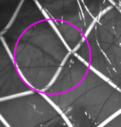
Heart surface frame during the experiment. Size is 208x208. White wires are electrode grid. The pink circle represents the approximate region of capture of the mechanical vortex (Sec. 9).

7. Proof of the proposed deep neural network scheme effectiveness with synthetic images

Figs. 6 a,b,c,d show bar charts showing the difference in results with the transformed images, that were produced with unsupervised deep network scheme, and the original frames for different frequency of displacement fields (coefficients ω and k in Eq. (6) and Eq. (7)) and degree of heterogeneity original pictures textures i.e. main correlation length (h, Eq. (5)). The quality as in prior section is evaluated with RMSE.

Figure 6.

Comparative bar charts for results obtained with and without transformation image texture method. a and b shows the results for simple harmonic fields case (Eq. (6)), c and d - for vortex fields case (Eq. (7)). ω and k represents the frequencies of fields, h is the main correlation length from Eq. (5).

Also, Figs. 7 a,b,c,d show comparative graphs that represents the dependence of RMSE on the degree of image texture heterogeneity. For a visual assessment of our ANN scheme effectiveness, you can look at Fig. 8 (a,b,c,d,e) and Fig. 9 (a,b,c,d,e) depicting simple harmonic and vortex displacement fields respectively which were obtained with both PIV and local DIC for image with h = 30 in Eq. (5)(Fig. 3).

Figure 7.

Comparative graphs for results obtained with and without transformation image texture method. a and b shows the results for simple harmonic fields case, c and d - for vortex fields case. ω and k represents the frequencies of fields (Eq. (6) and Eq. (7), h is the main correlation length from Eq. (5).

To make sure the results are not better just by varying the interrogation area, we varied the values of the PIV and DIC parameters and compared them with the results obtained using the texture transformation. The tables on Figs. 10 a,b show the results of this testing.

Figure 10.

Comparative table for different parameters (PIV, DIC). The values in the table show the mean RMSE with standard deviation for each displacement field across all four images with different main correlation length (h) from Eq. (5)Fig. 3. The best result highlighted with green. a - results for PIV, b - results for DIC.

8. Comparison with classical filters

The previous sections are devoted to studying the performance of our model on low-contrast images with different types and frequencies of displacement fields, as well as image textures. However, it is not possible to apply filtering to enhance pixel heterogeneity on these synthetic images due to the narrow range of pixel values. In this section, we conducted a comparative analysis of the performance of various filters that are often used to improve cross-correlation analysis methods (PIV, DIC) on photographs of cardiac tissue obtained from the experiment described in section 6. There were 8 different images in total (including the one from section 6 where mechanical vortex was fixed), each of which was deformed by three random fields generated using Perlin noise [51] (octaves 5, 6, 7). Each field was individual and unique. In total, the dataset have been included 24 pairs of images on which comparison was carried out. Four filters for comparing were chosen: CLAHE [48], Hessian [49] and Unsharp Masking [50]. The Figs. 12 a,b,c,d,e show an example for one photo. The table shows the results of calculating the RMSE and SSIM indexes, including those for the Grid Generator Output. The first two best results are highlighted with green. The Figs. 11 a,b,c show examples of displacement fields obtained by different methods.

Figure 12.

Image Example after applying different filters. a - Image without any filter, b - Image obtained with our method, c - Image obtained with CLAHE [48], d - Image obtained with Hessian [49] and e - Image obtained with Unsharp Masking [50].

Figure 11.

Different displacement fields examples (a,b,c) obtained using different filters. 1st line - PIV case, 2nd line - DIC case.

9. Mechanical vortex visualization

After performing the test calculations with synthetic images, our unsupervised deep network scheme was applied to 8 real frames depicting epicardium surface at the start of fibrillation that was registered with the ECG. Fig. 14a represents streamline graphs reflecting direction lines along displacements fields. With these streamline graphs one can see mechanical tracks of the formation and rotation of the electrical vortex (spiral wave) at the start of fibrillation while similar phenomena that was computed using single cross-correlation analysis (PIV) with integral CLAHE filter [44],[48] appear only on three frames (4,6 and 12 ms) (Fig. 14b) while we can see it on 4,6,8,12,14 and 16 milliseconds with using our model. The approximate region of this phenomenon is indicated in the Fig. 5. Important to note, the approximate size of the resulting vortex corresponds to the generated vortexes in Fig. 9a (k = 3) (i.e. our network was tested on vortices of such proportions).

Figure 14.

Streamline graphs of soft tissue epicardium deformation in the start of fibrillation. a - deformation obtained with transformed pixel texture of two consecutive images and PIV analysis, b - deformation obtained with single PIV. Picture size 60x60. The real vortex size is about 1 cm x 1 cm. The purple dot indicates the hypothetical center of the vortex.

10. Discussion

In this study the work of a novel unsupervised deep network scheme, which transform the pixel texture of image to improve the cross-correlation analysis, was evaluated. As a result of the experiments, the bandwidth related scale factor (γ) equaled 4 (Sec. 5, Fig. 4) has turned out to be the most optimal. With contiguous values, there is over-learning and under-learning respectively, as described in the work by M. Tancik [20].

With the evaluation of our ANN scheme effectiveness on low contrast images we can see that it improves the quality of analysis for both PIV and local DIC. Considering that filtering for such images is not applicable, it justifies the computational cost of the model (Fig. 8 a,b,c,d,e, Fig. 9 a,b,c,d,e). Figs. 7 a,b,c,d show that RMSE without using an ANN scheme grows depending on the degree of pixel heterogeneity, and with using it, it remains, approximately, at the same level. However, if the initial image structure is sufficiently heterogeneous (h = 3,11) in the Eq. (5)(Fig. 3), then our ANN can slightly degrade the quality of the cross-correlation analysis and gives a loss in some cases (Fig. 6 a,b,c,d). Figs. 6 a,b,c,d show that the gain from texture transformation is the greatest with greatest field with high frequencies both in the cases of a simple harmonic function and in the vortex function i.e. for unidirectional and multidirectional magnitudes (u,v). Moreover, the adequacy of using this method is confirmed in experiment with different parameters of PIV and DIC: enlargement and reduction of interrogation areas results in a larger error in receiving the displacement fields compared to using our model (table on Fig. 10).

In experiments on our dataset with comparing with classical filters, it can be concluded using average values and standard deviation of RMSE and SSIM that our model works on the level and better with one of the most popular filter CLAHE(Figs. 11 a,b,c and tables on Figs. 13 a,b). Remarkable, the indicators (RMSE and SSIM) of grid generator output are obviously higher that can be easily explained by the fact that cross-correlation analysis computes discrete values of the displacement field and then it interpolated (in this case, cubic). It results errors in measuring RMSE and SSIM while the grid generator determines the field pixel by pixel (Fig. 11 a,b,c). Nevertheless, it is obvious that these fields do not have gradient transitions, unlike the fields obtained using cross-correlation analysis and our model. This can be explained primarily by the smoothing effect of PIV and DIC and also the possible contribution of the image generator.

Figure 13.

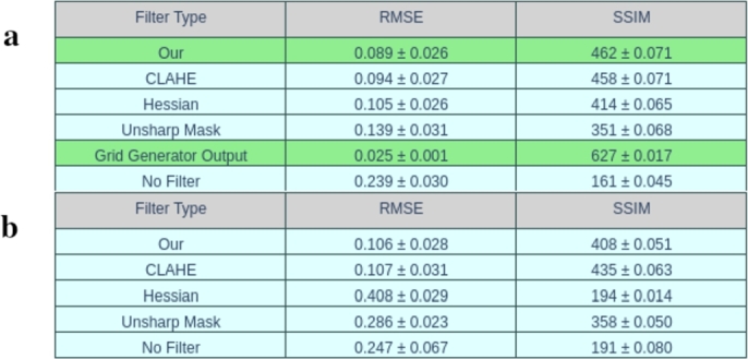
Comparative table for different filtering methods. The values in the table show the mean RMSE and SSIM with standard deviation for each displacement field across all 24 image pairs. The best result highlighted with green. a - results for PIV, b - results for DIC. The best result highlighted with green.

Despite the nuances described above, it can be concluded that in the course of this study, it was possible to catch a real mechanical track of a electrical vortex with our model more qualitatively (in some frames which was applied with CLAHE, there are no clear vortices). The reliability of the result was confirmed with testing this frames in section 8. In addition, it can be noted, the successive displacement fields in Figs. 14 a,b were read independently of each other but at the same time they have sufficient consistency. Finally, the appearance of the mechanical vortex (spiral wave) corresponds to other earlier studies about these phenomena but even with more details [14],[15],[16],[17],[18].

11. Conclusion

In the course of this study, encouraging results of experiments carried out with synthetic images for various displacement fields and images with different degree of pixel heterogeneity showed that our novel unsupervised deep neural network enables to improve the quality of cross-correlation analysis of images both usual and low contrast images where classical filters are not applicable. In comparison with classical filtering, our model works on the level and better with one of the most popular filter CLAHE. As a result of the study, a detailed mechanical track in epicardium was obtained for the first time from the movement of an electric spiral wave. The visualisation of this phenomenon is very useful for cardiophysiological research that aims to improve the treatment and diagnosis of cardiac fibrillation.

12. Further study and limitations

Taking into account the results obtained in the table and figure, the main work to improve the model should be directed to improving the image generator to obtain smoother displacement fields in the future, or a grid generator that could produce more realistic displacement fields with gradient transitions but not just optical flow (Fig. 11 a,b,c). In this work, the developed neural network showed encouraging results on a certain dataset. It turned out to be better than CLAHE, but it can be assumed that in a particular case it could be the other way around. It is also necessary to study this model further on other types of images and displacement fields, the values of which go beyond 1.5. Important to note, the optimal coefficient may vary slightly from sample to sample, which is also a small drawback.

Funding

The research funding from the Ministry of Science and Higher Education of the Russian Federation (Ural Federal University project within the Priority-2030 Program) is gratefully acknowledged.

CRediT authorship contribution statement

Daria Mangileva: Conceptualization, Formal analysis, Funding acquisition, Investigation, Methodology, Software, Validation, Visualization, Writing – original draft. Alexander Kursanov: Conceptualization, Data curation, Formal analysis, Investigation, Resources, Supervision, Validation, Writing – review & editing. Leonid Katsnelson: Conceptualization, Data curation, Formal analysis, Investigation, Project administration, Resources, Supervision, Validation, Writing – review & editing. Olga Solovyova: Conceptualization, Data curation, Formal analysis, Investigation, Project administration, Resources, Supervision, Validation, Writing – review & editing.

Declaration of Competing Interest

The authors declare that they have no known competing financial interests or personal relationships that could have appeared to influence the work reported in this paper.

Data availability statement

The data used in the study is available at the link: https://drive.google.com/drive/folders/16e0XDw38ZrhaPuhi2UyLujQe2P0X9PD3?usp=sharing

References

- 1.Adrian R.J. Particleimaging techniques for experimental fluid mechanics. Annu. Rev. Fluid Mech. 1991:261–304. [Google Scholar]
- 2.Sutton M.A., Wolters W., Peters W., Ranson W., McNeill S. Determination of displacements using an improved digital correlation method. Image Vis. Comput. 1983;1(3):133–139. [Google Scholar]
- 3.Palanca M., Tozzi G., Cristofolini L. The use of digital image correlation in the biomechanical area: a review. Int. Biomech. 2016;3(1):1–21. [Google Scholar]
- 4.Zhang D.S., Arola D.D. Applications of digital image correlation to biological tissues. J. Biomed. Opt. 2004;9(4):691–699. doi: 10.1117/1.1753270. [DOI] [PubMed] [Google Scholar]
- 5.Rizzuto E., Carosio S., Musarò A., Del Prete Z. 2015 IEEE International Symposium on Medical Measurements and Applications (MeMeA) Proceedings. IEEE; 2015. A digital image correlation based technique to control the development of a skeletal muscle engineered tissue by measuring its surface strain field; pp. 314–318. [Google Scholar]
- 6.Hamza O., Bengough A., Bransby M., Davies M., Hallett P. Biomechanics of plant roots: estimating localised deformation with particle image velocimetry. Biosyst. Eng. 2006;94(1):119–132. [Google Scholar]
- 7.Rossetti L., Kuntz L., Kunold E., Schock J., Müller K., Grabmayr H., Stolberg-Stolberg J., Pfeiffer F., Sieber S., Burgkart R., et al. The microstructure and micromechanics of the tendon–bone insertion. Nat. Mater. 2017;16(6):664–670. doi: 10.1038/nmat4863. [DOI] [PubMed] [Google Scholar]
- 8.Nobach H., Honkanen M. Two-dimensional Gaussian regression for sub-pixel displacement estimation in particle image velocimetry or particle position estimation in particle tracking velocimetry. Exp. Fluids. 2005;38(4):511–515. [Google Scholar]
- 9.Nobach H., Bodenschatz E. Limitations of accuracy in PIV due to individual variations of particle image intensities. Exp. Fluids. 2009;47(1):27–38. [Google Scholar]
- 10.Triconnet K., Derrien K., Hild F., Baptiste D. Parameter choice for optimized digital image correlation. Opt. Lasers Eng. 2009;47(6):728–737. [Google Scholar]
- 11.Reu P.L. Experimental and numerical methods for exact subpixel shifting. Exp. Mech. 2011;51(4):443–452. [Google Scholar]
- 12.Balakina-Vikulova N.A., Panfilov A., Solovyova O., Katsnelson L.B. Mechano-calcium and mechano-electric feedbacks in the human cardiomyocyte analyzed in a mathematical model. J. Physiol. Sci. 2020;70(1):1–23. doi: 10.1186/s12576-020-00741-6. [DOI] [PMC free article] [PubMed] [Google Scholar]
- 13.Orini M., Nanda A., Yates M., Di Salvo C., Roberts N., Lambiase P., Taggart P. Mechano-electrical feedback in the clinical setting: current perspectives. Prog. Biophys. Mol. Biol. 2017;130:365–375. doi: 10.1016/j.pbiomolbio.2017.06.001. [DOI] [PubMed] [Google Scholar]
- 14.Gray R.A., Jalife J., Panfilov A.V., Baxter W.T., Cabo C., Davidenko J.M., Pertsov A.M. Mechanisms of cardiac fibrillation. Science. 1995;270(5239):1222–1223. [PubMed] [Google Scholar]
- 15.Jalife J., Gray R. Drifting vortices of electrical waves underlie ventricular fibrillation in the rabbit heart. Acta Physiol. Scand. 1996;157(2):123–132. doi: 10.1046/j.1365-201X.1996.505249000.x. [DOI] [PubMed] [Google Scholar]
- 16.Gray R.A., Pertsov A.M., Jalife J. Spatial and temporal organization during cardiac fibrillation. Nature. 1998;392(6671):75–78. doi: 10.1038/32164. [DOI] [PubMed] [Google Scholar]
- 17.Witkowski F.X., Leon L.J., Penkoske P.A., Giles W.R., Spano M.L., Ditto W.L., Winfree A.T. Spatiotemporal evolution of ventricular fibrillation. Nature. 1998;392(6671):78–82. doi: 10.1038/32170. [DOI] [PubMed] [Google Scholar]
- 18.Christoph J., Chebbok M., Richter C., Schröder-Schetelig J., Bittihn P., Stein S., Uzelac I., Fenton F.H., Hasenfuß G., Gilmour R., Jr, et al. Electromechanical vortex filaments during cardiac fibrillation. Nature. 2018;555(7698):667–672. doi: 10.1038/nature26001. [DOI] [PubMed] [Google Scholar]
- 19.Mangileva D., Kursanov A., Tsvetkova A., Bernikova O., Ovechkin A., Grubbe M., Azarov J., Katsnelson L. Графикон-конференции по компьютерной графике и зрению. vol. 31. 2021. Preprocessing images algorithm without Gaussian shaped particles for PIV analysis and imaging vortices on the epicardial surface; pp. 519–528. [Google Scholar]
- 20.Tancik M., Srinivasan P., Mildenhall B., Fridovich-Keil S., Raghavan N., Singhal U., Ramamoorthi R., Barron J., Ng R. Fourier features let networks learn high frequency functions in low dimensional domains. Adv. Neural Inf. Process. Syst. 2020;33:7537–7547. [Google Scholar]
- 21.Dosovitskiy A., Fischer P., Ilg E., Hausser P., Hazirbas C., Golkov V., Van Der Smagt P., Cremers D., Brox T. Proceedings of the IEEE International Conference on Computer Vision. 2015. FlowNet: learning optical flow with convolutional networks; pp. 2758–2766. [Google Scholar]
- 22.Ilg E., Mayer N., Saikia T., Keuper M., Dosovitskiy A., Brox T. Proceedings of the IEEE Conference on Computer Vision and Pattern Recognition. 2017. FlowNet 2.0: evolution of optical flow estimation with deep networks; pp. 2462–2470. [Google Scholar]
- 23.Yu C., Bi X., Fan Y., Han Y., Kuai Lightpivnet Y. An effective convolutional neural network for particle image velocimetry. IEEE Trans. Instrum. Meas. 2021;70:1–15. [Google Scholar]
- 24.Cai S., Liang J., Zhou S., Gao Q., Xu C., Wei R., Wereley S., Kwon J.-s. Proceedings of the 13th International Symposium on Particle Image Velocimetry-ISPIV. 2019. Deep-PIV: a new framework of PIV using deep learning techniques. [Google Scholar]
- 25.Yang R., Li Y., Zeng D., Guo P. Deep DIC: deep learning-based digital image correlation for end-to-end displacement and strain measurement. J. Mater. Process. Technol. 2022;302 [Google Scholar]
- 26.Min H.-G., On H.-I., Kang D.-J., Park J.-H. Strain measurement during tensile testing using deep learning-based digital image correlation. Meas. Sci. Technol. 2019;31(1) [Google Scholar]
- 27.Boukhtache S., Abdelouahab K., Berry F., Blaysat B., Grediac M., Sur F. When deep learning meets digital image correlation. Opt. Lasers Eng. 2021;136 [Google Scholar]
- 28.Akçakaya M., Yaman B., Chung H., Ye J.C. Unsupervised deep learning methods for biological image reconstruction and enhancement: an overview from a signal processing perspective. IEEE Signal Process. Mag. 2022;39(2):28–44. doi: 10.1109/msp.2021.3119273. [DOI] [PMC free article] [PubMed] [Google Scholar]
- 29.Yu H., Yang L.T., Zhang Q., Armstrong D., Deen M.J. Convolutional neural networks for medical image analysis: state-of-the-art, comparisons, improvement and perspectives. Neurocomputing. 2021;444:92–110. [Google Scholar]
- 30.Xie Y., Takikawa T., Saito S., Litany O., Yan S., Khan N., Tombari F., Tompkin J., Sitzmann V., Sridhar S. vol. 41. Wiley Online Library; 2022. Neural Fields in Visual Computing and Beyond; pp. 641–676. (Computer Graphics Forum). [Google Scholar]
- 31.Rahaman N., Baratin A., Arpit D., Draxler F., Lin M., Hamprecht F., Bengio Y., Courville A. International Conference on Machine Learning, PMLR. 2019. On the spectral bias of neural networks; pp. 5301–5310. [Google Scholar]
- 32.Basri R., Galun M., Geifman A., Jacobs D., Kasten Y., Kritchman S. International Conference on Machine Learning, PMLR. 2020. Frequency bias in neural networks for input of non-uniform density; pp. 685–694. [Google Scholar]
- 33.Mildenhall B., Srinivasan P.P., Tancik M., Barron J.T., Ramamoorthi R., Ng R. NeRF: representing scenes as neural radiance fields for view synthesis. Commun. ACM. 2021;65(1):99–106. [Google Scholar]
- 34.Czerkawski M., Cardona J., Atkinson R., Michie C., Andonovic I., Clemente C., Tachtatzis C. Neural Knitworks: patched neural implicit representation networks. arXiv:2109.14406 arXiv preprint.
- 35.Anokhin I., Demochkin K., Khakhulin T., Sterkin G., Lempitsky V., Korzhenkov D. Proceedings of the IEEE/CVF Conference on Computer Vision and Pattern Recognition. 2021. Image generators with conditionally-independent pixel synthesis; pp. 14278–14287. [Google Scholar]
- 36.Bemana M., Myszkowski K., Seidel H.-P., Ritschel T. X-fields: implicit neural view-, light- and time-image interpolation. ACM Trans. Graph. 2020;39(6):1–15. [Google Scholar]
- 37.Li N., Thapa S., Whyte C., Reed A.W., Jayasuriya S., Ye J. Proceedings of the IEEE/CVF International Conference on Computer Vision. 2021. Unsupervised non-rigid image distortion removal via grid deformation; pp. 2522–2532. [Google Scholar]
- 38.Nam S., Brubaker M.A., Brown M.S. European Conference on Computer Vision. Springer; 2022. Neural image representations for multi-image fusion and layer separation; pp. 216–232. [Google Scholar]
- 39.Cao R., Liu F.L., Yeh L.-H., Waller L. 2022 IEEE International Conference on Computational Photography (ICCP) IEEE; 2022. Dynamic structured illumination microscopy with a neural space-time model; pp. 1–12. [Google Scholar]
- 40.A. Paszke, S. Gross, S. Chintala, G. Chanan, E. Yang, Z. DeVito, Z. Lin, A. Desmaison, L. Antiga, A. Lerer, Automatic differentiation in PyTorch.
- 41.Müller S., Schüler L., Zech A., Heße F. GSTools v1. 3: a toolbox for geostatistical modelling in Python. Geosci. Model Dev. 2022;15(7):3161–3182. [Google Scholar]
- 42.Webster R., Oliver M.A. John Wiley & Sons; 2007. Geostatistics for Environmental Scientists. [Google Scholar]
- 43.Olufsen S.N., Andersen M.E., Fagerholt E. μDIC: an open-source toolkit for digital image correlation. SoftwareX. 2020;11 [Google Scholar]
- 44.Thielicke W., Stamhuis E. PIVlab–towards user-friendly, affordable and accurate digital particle image velocimetry in MATLAB. J. Open Res. Softw. 2014;2(1) [Google Scholar]
- 45.Belloni V., Ravanelli R., Nascetti A., Di Rita M., Mattei D., Crespi M. py2DIC: a new free and open source software for displacement and strain measurements in the field of experimental mechanics. Sensors. 2019;19(18):3832. doi: 10.3390/s19183832. [DOI] [PMC free article] [PubMed] [Google Scholar]
- 46.Azarov J.E., Ovechkin A.O., Vaykshnorayte M.A., Demidova M.M., Platonov P.G. Prolongation of the activation time in ischemic myocardium is associated with J-wave generation in ECG and ventricular fibrillation. Sci. Rep. 2019;9(1):1–8. doi: 10.1038/s41598-019-48710-3. [DOI] [PMC free article] [PubMed] [Google Scholar]
- 47.Feng B.Y., Varshney A. Proceedings of the IEEE/CVF International Conference on Computer Vision. 2021. SIGNET: efficient neural representation for light fields; pp. 14224–14233. [Google Scholar]
- 48.Pizer S.M., Amburn E.P., Austin J.D., Cromartie R., Geselowitz A., Greer T., ter Haar Romeny B., Zimmerman J.B., Zuiderveld K. Adaptive histogram equalization and its variations. Comput. Vis. Graph. Image Process. 1987;39(3):355–368. [Google Scholar]
- 49.Magnus J.R., Neudecker H. John Wiley & Sons; 2019. Matrix Differential Calculus with Applications in Statistics and Econometrics. [Google Scholar]
- 50.Polesel A., Ramponi G., Mathews V. Image enhancement via adaptive unsharp masking. IEEE Trans. Image Process. 2000;9(3):505–510. doi: 10.1109/83.826787. [DOI] [PubMed] [Google Scholar]
- 51.Perlin K. An image synthesizer. ACM Siggraph Comput. Graph. 1985;19(3):287–296. [Google Scholar]
Associated Data
This section collects any data citations, data availability statements, or supplementary materials included in this article.