

Abstract
Chronic urticaria is a chronic skin disease that affects up to 1% of the general population worldwide, with chronic spontaneous urticaria accounting for more than two-thirds of all chronic urticaria cases. The Urticaria Activity Score (UAS) is a dynamic severity assessment tool that can be incorporated into daily clinical practice, as well as clinical trials for treatments. The UAS helps in measuring disease severity and guiding the therapeutic strategy. However, UAS assessment is a time-consuming and manual process, with high interobserver variability and high dependence on the observer. To tackle this issue, we introduce Automatic UAS, an automatic equivalent of UAS that deploys a deep learning, lesion-detecting model called Legit.Health-UAS-HiveNet. Our results show that our model assesses the severity of chronic urticaria cases with a performance comparable to that of expert physicians. Furthermore, the model can be implemented into CADx systems to support doctors in their clinical practice and act as a new end point in clinical trials. This proves the usefulness of artificial intelligence in the practice of evidence-based medicine; models trained on the consensus of large clinical boards have the potential of empowering clinicians in their daily practice and replacing current standard clinical end points in clinical trials.
Introduction
Urticaria is a very common disease characterized by erythematous, edematous, itchy, and transient plaques that involve the skin and mucous membranes. It can be classified into subtypes, such as acute spontaneous urticaria, chronic spontaneous urticaria, chronic inducible urticaria, and episodic chronic urticaria (CU). Urticaria can be related to factors such as infections, drugs, food, psychogenic factors, and respiratory allergens, but sometimes it can also be idiopathic. Clinical manifestations of the disease involve red, swollen, and itchy plaques. The lesions usually recede spontaneously within 2 to 3 hours without leaving a trace (Kayiran and Akdeniz, 2019).
Diagnosis of CU is usually performed through clinical observation. In other words, the assessment of the severity is performed through manual scoring systems that are filled in subjectively. The European Academy of Allergy and Clinical Immunology, the European Global Allergy and Asthma Network, the European Dermatology Forum, and the World Allergy Organization Guideline have agreed on a list of relevant items to be considered when assessing the condition. In all cases, the literature suggests that analyzing a detailed history is essential when diagnosing and treating urticaria. On the one hand, to make a proper assessment, clinicians should know the frequency of episodes, circumstances of onset, triggers, duration of individual lesions, the pattern of recurrence, duration of attacks, whether lesions are itchy or painful, and whether episodes are associated with systemic symptoms. On the other hand, beyond diagnosis, it is also essential to document the response to the treatment because there is a wide range of therapeutic options. Unfortunately, there are no reliable markers to diagnose urticaria and measure its activity. Therefore, the activity of urticaria can only be measured using scoring systems, which are mainly filled manually on paper sheets or through certain apps such as UrCare or UrticariApp.
The most commonly used scoring system is the Urticaria Activity Score (UAS), which can also be used for 7 consecutive days, in which case, it is referred to as UAS7. There are alternative scoring systems, such as the Urticaria Control Test, the Chronic Urticaria Quality of Life Questionnaire, the Patient’s Global Assessment of Disease Severity, and the Physician’s Global Assessment of Disease Control, which work in a similar manner. Ultimately, it can be said that pen and paper–based questionnaires play a central role in the management of urticaria. So much so that self-reported questionnaires are the main, if not the only, prospective measurement tools and the most accepted method of assessing CU and assigning treatment to patients.
The most indisputable limitation of manual scoring systems is the inherent difficulty of human beings to quantify parameters in an objective, stable, and precise manner. Humans have a limited ability to count hives and quantify the surface area of a lesion or the redness of an area.
This human limitation in parameter estimation is also reflected in the effort and time required to complete the urticaria activity questionnaires, which end up being a very unrewarding task for patients and may result in poor adherence.
Scoring systems classify disease severity using a limited range of scores, with three or four categories, such as none, mild, moderate, and severe in the case of the UAS. All these questionnaires have a very high minimum detectable change, as they are discrete ranges rather than continuous scales.
Finally, these questionnaires are susceptible to bias. This is especially true for cases in which the patient knows that the treatment they receive will be determined by the information they provide. In addition, because of the asynchronous nature of the reported measure, the clinical team lacks the means to ensure that the values reported by the patient are chronologically accurate or simply truthful, which precludes external verification.
Because the concept of “artificial intelligence” was introduced in 1956, it has led to numerous technological innovations in human medicine and is quickly becoming an integral part of modern health care. Convolutional neural networks (CNNs) have several applications, such as classification, segmentation, object detection, and even synthetic data generation. Many studies have applied classification methods to perform diagnosis using clinical, dermatoscopic, and histopathological imaging, whereas others applied segmentation CNNs for lesion surface estimation and quantification (Li et al., 2021). Wu et al. (2019) developed an object detection method to count acne lesions for the first time in the dermatological field.
In this work, we propose the Automatic UAS (AUAS), an automatic version of the objective part of the UAS that applies CNNs to count hives automatically. The goal is to assist clinicians in filling scoring systems such as the UAS in a more objective manner and quicker, which could improve health outcomes and provide high-quality end points to measure the effectiveness of the treatments for urticaria.
Results
Annotation variability assessment
To further understand annotation performance and label reliability, we used the F1 score (F1-box and F1-mask) and mean absolute error (MAE) to assess both interobserver and intraobserver variability. We also computed Krippendorff alpha for both lesion counting and overall severity assessment.
Intraobserver variability
The results of this analysis are presented in Table 1. In terms of bounding box annotation agreement (i.e., the F1-box score), the results were not compelling because we obtained an average score of 0.096, suggesting that there was maximum variability. However, the F1-mask scores remained high (with an average score of 0.789). This helped us understand the results a bit better, which will be covered in Discussion. The lesion counting variability in terms of MAE was low (1.81 hives on average).
Table 1.
Intraobserver Annotation Variability Analysis
| Specialist | F1-Box Score | F1-Mask Score | MAE |
|---|---|---|---|
| A | 0.070 | 0.831 | 1.714 |
| B | 0.167 | 0.884 | 1.286 |
| C | 0.062 | 0.692 | 1.667 |
| D | 0.127 | 0.694 | 1.095 |
| E | 0.055 | 0.846 | 3.286 |
| Mean | 0.096 | 0.789 | 1.810 |
Abbreviation: MAE, mean absolute error.
For each specialist, we calculated the F1 scores (F1-box and F1-mask) and absolute error in every image pair and then averaged the results.
The results from this analysis must be interpreted with caution. As we stated while describing the dataset, this subset of 21 image pairs mostly contains cases in which lesion boundaries are very difficult to distinguish. Therefore, this analysis has been useful to point out the challenges of counting hives in difficult cases and the impact of distance and perspective in image-based urticaria severity assessment, but it does not summarize overall intraobserver variability. Counting hives on all the remaining images of urticaria may have been easier, but we did not have such pairs of close-up and general images to conduct the analysis to prove it.
Interobserver variability
This analysis did not require any preprocessing as in the intraobserver variability experiment. For each specialist and image, we calculated the F1 scores and MAEs among annotations and finally aggregated the results. Tables 2 and 3 show the similarity among specialists using the F1 scores in the whole dataset. In terms of actual lesion counting (MAE), the disagreement among observers is more evident (Table 4). Krippendorff alpha was 0.826 for the task of hive counting and 0.603 for severity assessment.
Table 2.
Interobserver Annotation Variability Analysis in the 313 Urticaria Images Using the F1-Box Score between Image labels
| Specialist | A | B | C | D | E | Average F1-Cox Score |
|---|---|---|---|---|---|---|
| A | - | 0.455 | 0.383 | 0.419 | 0.476 | 0.433 |
| B | 0.455 | - | 0.390 | 0.406 | 0.563 | 0.454 |
| C | 0.383 | 0.39 | - | 0.360 | 0.388 | 0.380 |
| D | 0.419 | 0.406 | 0.360 | - | 0.413 | 0.400 |
| E | 0.476 | 0.563 | 0.388 | 0.413 | - | 0.460 |
The F1-box score between specialists was calculated for every image and then averaged the results. The last column is the average of each specialist’s F1-box score.
Table 3.
Interobserver Annotation Variability Analysis in the 313 Urticaria Images Using the F1-Mask Score between Image Labels
| Specialist | A | B | C | D | E | Average F1-Mask Score |
|---|---|---|---|---|---|---|
| A | - | 0.677 | 0.619 | 0.614 | 0.693 | 0.651 |
| B | 0.677 | - | 0.629 | 0.637 | 0.746 | 0.672 |
| C | 0.619 | 0.629 | - | 0.574 | 0.629 | 0.613 |
| D | 0.614 | 0.637 | 0.574 | - | 0.636 | 0.615 |
| E | 0.693 | 0.746 | 0.629 | 0.636 | - | 0.676 |
For every image, we calculated the F1-mask score between specialists and then averaged the results. The last column is the average of each specialist’s F1-mask score.
Table 4.
Interobserver Annotation Variability Analysis in the Urticaria Images (313 of 353): MAE
| Specialist | A | B | C | D | E | Average MAE |
|---|---|---|---|---|---|---|
| A | - | 10.37 | 6.04 | 4.19 | 10.49 | 7.52 |
| B | 10.37 | - | 7.33 | 9.45 | 6.52 | 8.17 |
| C | 6.04 | 7.33 | - | 5.69 | 7.49 | 6.39 |
| D | 4.19 | 9.45 | 5.69 | - | 10.14 | 7.12 |
| E | 10.49 | 6.52 | 7.49 | 10.14 | - | 8.41 |
Abbreviation: MAE, mean absolute error.
For every image, we calculated the absolute error between each specialist’s lesion counts and then averaged the results. The last column is the average of each specialist.
The results from these tables suggest that despite being an overall noisy dataset, specialists may be agreeing on the rough location of lesions but disagreeing on their extent. Another source of disagreement may be that while specialists tend to label a close group of lesions as a single box, others prefer to be more precise and label each smaller lesion separately (Figure 1).
Figure 1.
Example of an annotated image with noisy labels. Inconsistent labeling happened in some difficult cases, where some specialists may tag each smaller hive individually, whereas some specialists may prefer to consider the whole region as a single lesion. Image source: Interactive Dermatology Atlas.
Model performance
Hive detection
Training every model architecture on every fold resulted in 20 experiments in total. Table 5 summarizes the performance of Legit.Health-UAS-HiveNet with different architectures in our 4-fold cross-validation scenario. In general, all the versions showed a similar performance taking into account the SD. However, if we consider model size and inference speed, the winning model was YOLOV5m, which would provide faster performance than the actual best model (YOLOv5x) when integrated in the CADx system.
Table 5.
Average Detection Performance of Each YOLOv5 Architecture
| Model | P | R | F1-Box | mAP@0.5 | Time (s) |
|---|---|---|---|---|---|
| yolov5n | 0.647 ± 0.045 | 0.564 ± 0.034 | 0.602 ± 0.036 | 0.604 ± 0.054 | 0.0335 ± 0.0909 |
| yolov5s | 0.669 ± 0.045 | 0.578 ± 0.039 | 0.620 ± 0.039 | 0.615 ± 0.049 | 0.0337 ± 0.0906 |
| yolov5m | 0.684 ± 0.039 | 0.571 ± 0.054 | 0.622 ± 0.047 | 0.617 ± 0.064 | 0.0354 ± 0.0905 |
| yolov5l | 0.682 ± 0.071 | 0.570 ± 0.046 | 0.621 ± 0.054 | 0.618 ± 0.068 | 0.0371 ± 0.0897 |
| yolov5x | 0.681 ± 0.043 | 0.578 ± 0.055 | 0.624 ± 0.044 | 0.621 ± 0.065 | 0.0390 ± 0.0895 |
Abbreviations: mAP@0.5, mean average precision; P, precision; R, recall.
Precision (P), recall (R), F1-box score, and mean average precision (mAP@0.5) on the Legit.Health-CU-UAS-V1 dataset with 4-fold cross-validation (mean ± SD). We also include the average inference time per image (including all the image preprocessing required to feed the model). This F1-box score is computed using the total number of ground truth and predicted boxes of all the dataset, not per image.
Each of these 20 models (one for each split and architecture) was validated on their corresponding validation sets using a range of confidence thresholds while keeping the intersection over union (IoU) threshold at 0.60 for nonmaximum suppression (NMS) and 0.50 for comparisons to the ground truth. The best confidence threshold of each model was the one that resulted in the highest F1 score. The optimal confidence threshold for each model can be found in Table 6. The best overall confidence threshold of each architecture (YOLOv5n, YOLOv5s, YOLOv5m, YOLOv5l, and YOLOv5x) was the threshold that got the highest F1 score on average. Figure 2 presents the average performance of each model in terms of F1 score. This figure is useful to determine the threshold to be used at inference time from which we can conclude that a confidence threshold between 0.40 and 0.50 would offer optimal performance for all architectures.
Table 6.
Best Confidence Thresholds
| Model | Fold 1 | Fold 2 | Fold 3 | Fold 4 |
|---|---|---|---|---|
| yolov5n | 0.27 | 0.36 | 0.38 | 0.39 |
| yolov5s | 0.44 | 0.27 | 0.37 | 0.48 |
| yolov5m | 0.36 | 0.43 | 0.41 | 0.56 |
| yolov5l | 0.24 | 0.33 | 0.39 | 0.56 |
| yolov5x | 0.42 | 0.23 | 0.52 | 0.41 |
The best confidence threshold is the one that achieves the highest F1 score in the validation set. The intersection over union threshold for nonmaximum suppression was always set to 0.60.
Figure 2.

Selection of the best confidence threshold based on the F1 versus confidence plot. For each model architecture, we averaged the F1 score plots (one for each split) to find which threshold produces the highest F1 score.
To provide further detail regarding model performance on each level of severity, Table 7 shows the average F1-box score of each model on every severity group (none, mild, moderate, and severe urticaria). We compared model performance to the performance of the specialists by computing the F1-box score between each specialist and the ground truth (Table 8).
Table 7.
F1-Box Score of Each Model, Separated by Severity (4-Fold Cross-Validation)
|
Model |
F1-Box Score |
|||
|---|---|---|---|---|
| None | Mild | Moderate | Severe | |
| yolov5n | 0.84 ± 0.17 | 0.53 ± 0.04 | 0.59 ± 0.06 | 0.53 ± 0.06 |
| yolov5s | 0.85 ± 0.17 | 0.53 ± 0.04 | 0.60 ± 0.08 | 0.59 ± 0.10 |
| yolov5m | 0.87 ± 0.14 | 0.54 ± 0.04 | 0.61 ± 0.10 | 0.55 ± 0.09 |
| yolov5l | 0.84 ± 0.12 | 0.54 ± 0.05 | 0.59 ± 0.08 | 0.56 ± 0.08 |
| yolov5x | 0.93 ± 0.05 | 0.56 ± 0.05 | 0.60 ± 0.09 | 0.56 ± 0.07 |
Each validation split was separated into groups of images according to the ground truth severity. The F1-box score was then computed for every image of the group and averaged. We present the aggregated results of all folds.
Table 8.
Average F1-Box Score of each Specialist Versus the Consensus (Ground Truth)
|
Specialist |
F1-Box Score |
||
|---|---|---|---|
| Mild | Moderate | Severe | |
| A | 0.65 | 0.58 | 0.53 |
| B | 0.44 | 0.33 | 0.23 |
| C | 0.63 | 0.55 | 0.41 |
| D | 0.51 | 0.37 | 0.38 |
| E | 0.62 | 0.52 | 0.49 |
| Mean | 0.57 | 0.47 | 0.41 |
To be comparable to the models, we computed the F1-box score of each specialist to the ground truth in every validation split and then obtained the mean and SD. The “none” category (i.e., the healthy images) has been omitted because they were not annotated, and their agreement on this category is not required because it is always 1.
Severity assessment based on lesion counting
We used the best confidence threshold of each model to obtain the total number of predicted hives and the corresponding severity in every image of their validation splits. We then conducted a Bland-Altman analysis on every fold to evaluate the counting bias of each model. The results of this analysis using the winning model (yolov5m) are presented in Figure 3. Krippendorff alpha values for each task (lesion counting and severity assessment) are summarized in Table 9, and MAE is summarized in Table 10.
Figure 3.

Bland-Altman analysis of the winning architecture (YOLOv5m). We generated the Bland-Altman plot for every model of this architecture (each one trained and validated on a different fold).
Table 9.
Krippendorff Alpha for Hive Counting and Severity Assessment
| Model | Lesion Counting | Severity Assessment |
|---|---|---|
| yolov5n | 0.890 ± 0.031 | 0.805 ± 0.051 |
| yolov5s | 0.909 ± 0.039 | 0.795 ± 0.021 |
| yolov5m | 0.895 ± 0.032 | 0.715 ± 0.072 |
| yolov5l | 0.888 ± 0.055 | 0.760 ± 0.026 |
| yolov5x | 0.898 ± 0.067 | 0.773 ± 0.088 |
After computing these coefficients for each model on every fold, we aggregated the results (mean and SD).
Table 10.
Regression Metrics of Each YOLOv5 Model in their Validation Splits, Separated by Severity
|
Model |
MAE |
|||
|---|---|---|---|---|
| None | Mild | Moderate | Severe | |
| yolov5n | 0.16 ± 0.17 | 2.75 ± 0.52 | 7.74 ± 1.28 | 14.70 ± 3.70 |
| yolov5s | 0.23 ± 0.32 | 2.69 ± 0.31 | 7.45 ± 1.83 | 11.90 ± 5.83 |
| yolov5m | 0.16 ± 0.20 | 2.42 ± 0.34 | 8.68 ± 1.68 | 22.00 ± 6.15 |
| yolov5l | 0.19 ± 0.17 | 2.60 ± 0.44 | 8.65 ± 1.46 | 15.40 ± 8.49 |
| yolov5x | 0.08 ± 0.05 | 2.44 ± 0.42 | 7.805 ± 2.9 | 12.83 ± 8.00 |
Abbreviation: MAE, mean absolute error.
The method for computing the metric in severity groups was the same as for Table 9. The results presented are the mean and SD of all folds.
With regard to classification metrics, Table 11 present the performance (balanced accuracy [BAC]) of each model. The classification performance of each specialist compared with the ground truth is summarized in Table 12.
Table 11.
BAC of Each Model (4-Fold Cross-Validation)
| Model | BAC |
|---|---|
| yolov5n | 0.71 ± 0.07 |
| yolov5s | 0.72 ± 0.05 |
| yolov5m | 0.58 ± 0.04 |
| yolov5l | 0.69 ± 0.05 |
| yolov5x | 0.70 ± 0.10 |
Abbreviation: BAC, balanced accuracy.
The classification task consists of correctly labeling each image as “none,” “mild,” “moderate,” or “severe” urticaria based on the number of hives detected by the model (itch severity was not taken into account in the present work). For each fold, we calculated BAC and then aggregated the results (mean and SD).
Table 12.
Classification Metrics of the Specialists: BAC
| Specialist | BAC |
|---|---|
| A | 0.87 |
| B | 0.89 |
| C | 0.74 |
| D | 0.75 |
| E | 0.88 |
| Mean | 0.83 |
Abbreviation: BAC, balanced accuracy.
For each specialist, we compared their severity answers on every image (based on how many hives they labeled) to the consensus (ground truth).
Skin tone and model performance
To understand model performance in images of the patients with urticaria with dark skin, we separated some of the metrics by skin tone into light and dark skin. Table 13 shows overall behavior in terms of F1-box, BAC, and MAE for both skin tones.
Table 13.
F1-Box Score, BAC and MAE for Different Skin Tones
|
Model |
Light Skin |
Dark Skin |
||||
|---|---|---|---|---|---|---|
| F1-Box | BAC | MAE | F1-Box | BAC | MAE | |
| yolov5n | 0.57 ± 0.04 | 0.70 ± 0.07 | 4.10 ± 0.41 | 0.59 ± 0.09 | 0.87 ± 0.089 | 1.66 ± 0.69 |
| yolov5s | 0.59 ± 0.04 | 0.71 ± 0.07 | 3.95 ± 0.55 | 0.575 ± 0.13 | 0.82 ± 0.12 | 1.55 ± 0.62 |
| yolov5m | 0.60 ± 0.06 | 0.59 ± 0.04 | 4.42 ± 0.83 | 0.525 ± 0.12 | 0.76 ± 0.12 | 1.51 ± 0.75 |
| yolov5l | 0.60 ± 0.05 | 0.70 ± 0.04 | 4.05 ± 0.71 | 0.53 ± 0.03 | 0.78 ± 0.09 | 1.50 ± 0.57 |
| yolov5x | 0.61 ± 0.05 | 0.70 ± 0.10 | 3.82 ± 0.79 | 0.53 ± 0.13 | 0.84 ± 0.06 | 1.47 ± 0.82 |
Abbreviations: BAC, balanced accuracy; MAE, mean absolute error.
The dark skin images of our current dataset contain only healthy skin or mild urticaria, hence the superior results. We present the aggregated results of all folds (mean and SD).
Discussion
Our earliest exploration of the annotations (Table 14) suggested that urticaria assessment can be affected by interobserver variability. This has been further explored in Table 2, Table 3, confirming the presence of strong interobserver variability. Even under such variability, all specialists tended to agree on the actual number of hives, as indicated by the high Krippendorff alpha coefficient (0.826). However, variability has an impact on their agreement in terms of severity assessment (0.603) because large variations in hive counts can lead to a jump to the next or previous stage of severity (Table 15). Moreover, our intraobserver variability analysis, despite being limited, has shown that the assessment of the same specialist can change drastically on looking at the same case from a different point of view (Table 1) or at least in the presence of severe urticaria.
Table 14.
Annotation Summary of the Urticaria Images (313 of the Final Set of Images): Minimum, Maximum, and Average Number of Hives Detected in an Image and the Total Number of Annotations Generated Per Observer
|
Specialist |
Hives |
|||
|---|---|---|---|---|
| Min | Max | Average | Total | |
| A | 0 | 148 | 23 | 7682 |
| B | 0 | 115 | 15 | 5007 |
| C | 1 | 67 | 12 | 4031 |
| D | 0 | 82 | 12 | 3949 |
| E | 0 | 178 | 20 | 6534 |
Abbreviations: Max, maximum; Min, minimum.
Table 15.
UAS (Urticaria Activity Score)
| Itch Severity Score | Itch Severity (Once Every 24 h) | Hives Severity Score | Number of Hives per 24 h |
|---|---|---|---|
| 0 | None | 0 | 0 |
| 1 | Mild (present but not annoying or troublesome) | 1 | <20 |
| 2 | Moderate (troublesome but does not interfere with normal daily activity or sleep | 2 | 20-50 |
| 3 | Intense (interferes with normal daily activity or sleep) | 3 | >50 |
Overall, our variability analysis suggests that hive counting can become a time-consuming task, and specialists may prefer to estimate the approximate number of hives instead of actually counting them one by one and their annotations for this work may be reflecting this behavior (Figure 1).
Observer variability poses a problem for obtaining reliable manual counting reports from both the patient and the doctor. In contrast to manually calculating the hive number and using only four categories, Legit.Health-UAS-HiveNet aims for objective and quick evaluation by counting hives individually and automatically filling the objective part of the UAS (AUAS) and should therefore be developed further as an alternative method to human assessment. Despite the current dataset size, the hive detection metrics summarized in Table 5 are promising and show the potential of deep learning methods as a means of automatic hive counting.
In terms of severity assessment, BAC of Legit.Health-UAS-HiveNet was, on average, lower than that of the specialists, but the results are compelling. Lower metrics compared with those of the specialists was an expected outcome because class imbalance made every split has a different ratio of each severity and hinder a model’s ability to generalize to severe cases. In fact, the Bland-Altman plots presented in Figure 3 for the best architecture (YOLOv5m) reveal that all models are biased to some degree. This Bland-Altman analysis also suggests that measurement difference tends to increase with the number of hives, that is more the number of hives, the more severe the case is, and therefore more likely it will be to have overlapping of irregular hives.
Another reason behind the current performance (of both models and specialists) on images of severe urticaria is the appearance of the lesions. Most of the images of severe urticaria contain either lesions of very irregular shapes or many small lesions close to each other, which led to extremely noisy and heterogeneous labels. With some images of severe cases containing >100 hives (Table 14), it was expected that some specialists would prefer to annotate bigger boxes and avoid such extremely high levels of detail. This can be also the case in full-body images, in which small hives may tend to be grouped and be considered as a single lesion. Apart from lesion shape, we have also observed high variability in terms of image intensity and contrast, which may have also affected the annotation process (including the assignment of the exact Fitzpatrick Scale). All these factors made our knowledge unification algorithm produce inaccurate labels in these difficult cases which, when compared with the actual predictions, resulted in a higher MAE.
Figure 1 depicts an example of such a scenario, in which because of having a small clinical annotation team, noisy labels may have a remarkable impact on the final labels, which are obtained from the weighted sum of all doctors’ annotations. Such limitation will be overcome with a bigger annotation team, owing to an increased density of labels at each potential lesion, spurious inaccurate boxes, such as the presented in Figure 1, would be attenuated when generating the overall Gaussian map. We also believe that it would be possible to reduce the effect of both lesion and skin appearance by working on different color spaces not only at training time but also earlier during annotation; giving the specialists different views of the same image might boost annotation performance. Another future improvement is to work with images of enough resolution and quality, which was not always possible at this point. Future work will be required to acquire new images instead of relying on atlases. Such new images will be taken with a clear goal, which is to guarantee a successful and detailed annotation to obtain more reliable labels.
However, despite all the challenges in this work, the results presented in Tables 5 and 8 give us valuable insights; looking at the F1-box score, we can conclude that the models have similar performance to that of the specialists.
Regarding the knowledge unification algorithm, comparing every possible pair of annotations could become intractable if all the images had a high number of boxes per specialist, which would make our current method time-consuming and extremely slow. For that reason, we suggest using the F1-mask score instead of the F1-box when dealing with urticaria datasets with an even large number of annotations. Despite the fact that a semantic segmentation metric is not suitable for object detection, we believe it could serve as a fast alternative to approximate the ideal annotation score without the inconveniences of long processing times.
Last but not the least, another limitation of this study was image demographics. Although our dataset already contained examples with dark skin tones, the majority of pictures present similar demographics (Caucasian). We decided to assess hive detection performance on these dark skin images and include some examples in the figures. Table 13 compares model performance on light and dark skin. The output of a YOLOv5m model on a validation image of dark skin is presented in Figure 4. On these dark skin images, it is easier to spot hives based on how light reflects the skin (detecting the bumps), whereas erythema is not as easy to observe on lighter color skin. This may make it easier for a human to annotate light skin images (and therefore for a model to learn and generalize). However, the average performance of the current models on dark skin is compelling, probably because despite being more difficult to spot, they present mild or moderate urticaria, which makes them easier to be annotated without noise. In conclusion, in future iterations of this study, apart from recruiting a larger annotation team and using a larger dataset, we will also include as many cases of every skin tone as possible to overcome any bias related to pigmentation.
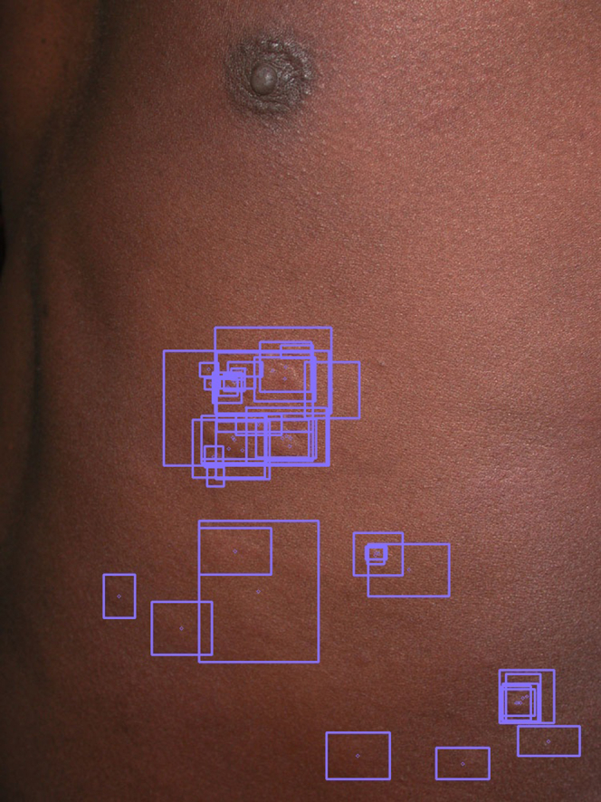
Figure 4.

Validation of Legit.Health-UAS-HiveNet on dark skin images. Predictions of YOLOv5m (green) on a validation image of fold 2 compared with the ground truth (purple). The model is capable of detecting several hives but still misses some of them and yields a false positive. Image source: Interactive Dermatology Atlas.
Materials and Methods
Dataset and annotations
To conduct this retrospective, noninterventional study, we collected and annotated images from several dermatology atlases to obtain a new dataset called Legit.Health-CU-UAS to train and test the performance of the hive counting model.
The initial dataset consisted of 334 images of patients with CU on different body parts and 40 images of healthy individuals with different skin tones. This resulted in an initial dataset size of 374 images. The images have a minimum size of 170 × 191 pixels, an average size of 696 × 1,008 pixels, and a maximum size of 5,464 × 8,192 pixels. We manually reviewed every image to estimate the total number of subjects to correctly split the data into training and validation sets. This exploration revealed 248 different subjects.
The dataset was annotated by a board of five expert dermatologists who frequently care for patients with urticaria. The 40 skin images from healthy individuals did not require annotation because they did not contain any lesions at all. After an initial review of the images of the skin of patients with urticaria (334), all specialists agreed by majority vote on removing 21 images from this set because they did not meet the following preestablished technical requirements: some images were incorrectly labeled (they were not actual cases of urticaria) and others, despite being of urticaria, were not in the scope of this project (e.g., urticaria pigmentosa). This reduced the number of urticaria images from 334 to 313. Cleaning the dataset resulted in a final dataset size of 353 images (313 of urticaria and 40 of healthy skin) and 231 subjects.
From this final set of 353 images, we observed that 21 images were either close-up views of other images or were the same pictures but taken from slightly different angles and distances. This became convenient for assessing intraobserver variability. However, it is important to point out that most of the images of this subset corresponded to difficult examples of urticaria in which lesion boundaries are difficult to define. This poses a limit to the power of this variability analysis, which will be discussed in subsequent sections.
The demographics of the final dataset are presented in Table 16. We have the following four groups of subjects: patients with urticaria with dark skin, healthy individuals with dark skin, patients with urticaria with light skin, and healthy individuals with light skin. We split each of the patient groups into four folds. The presence of urticaria in patients with darker skin tones, although underrepresented, made it possible to conduct a preliminary analysis of model performance on dark skin. For these patients with urticaria who had dark skin, because we had exactly 4 subjects, we decided to invert the splitting method in which for each fold, we assigned 1 subject to the training set and 3 subjects to the validation set. We did this on purpose because we wanted to assess model performance on all folds when images of patients with urticaria with darker skin tones are underrepresented in the training set. The distribution of the data for this 4-fold cross-validation experiment is presented in Table 17. Being able to separate images according to subject made it possible to stratify the training and validation sets in a manner that prevented data leakage. To label the skin as “dark” or “light,” we manually reviewed every image by comparing it to the Fitzpatrick scale color references. The lower scale values (1, 2, and 3) were considered light skin, and the remaining values (4, 5, and 6) were treated as dark skin.
Table 16.
Patient Demographics of the Legit.Health-CU-UAS Dataset after Annotating and Reviewing the Images
| Skin Tone | Urticaria | Healthy |
|---|---|---|
| Dark | 4 | 7 |
| Light | 192 | 33 |
Table 17.
Summary of Our 4-Fold Cross-Validation Experiment
| Fold | Training Images | Validation Images | Total Training Subjects | Total Validation Subjects | Dark Skin Subjects in the Training Set | Dark Skin Subjects in the Validation Set |
|---|---|---|---|---|---|---|
| 1 | 262 | 91 | 171 | 60 | 5 | 6 |
| 2 | 256 | 97 | 171 | 60 | 5 | 6 |
| 3 | 245 | 108 | 171 | 60 | 5 | 6 |
| 4 | 280 | 73 | 172 | 59 | 6 | 5 |
All four patient groups were split into training and validation four times.
Regarding the annotation carried out by the expert specialists on the urticaria images, Table 14 summarizes each specialist’s performance. The annotation task consisted of drawing a box around each hive, hereafter referred to as a “bounding box.” Figure 1 shows an example of an annotated image with its corresponding bounding boxes from all annotators. The experts had no time limit to perform the task and could revisit the annotation any number of times, and they received prior training on how to properly annotate lesions. Itch severity was not considered in this work because it was not possible to obtain this subjective variable from the selected images. Once the annotation of an image was completed, it was possible to obtain the severity based on the number of hives labeled, excluding the itch severity. Figure 5 shows the distribution of severity for each specialist.
Figure 5.

Severity distribution of the 313 urticaria images, according to each specialist.
Ground truth
To make annotations more accurate and reliable for supervised training, clinical imaging datasets must be reviewed by a large number of specialists. However, this presents a great challenge: each specialist labels differently, which very often results in annotations that are far from similar and sometimes even mutually exclusive (Figure 1). In this particular scenario, in which one image can contain >100 annotations, merging labels in a recursive process (e.g., finding overlapping boxes and merging them recursively) can become intractable. This led us to develop a more efficient alternative. To the best of our knowledge, literature on clinical label denoising in object detection is sparse (Khudorozhkov et al., 2018; Welikala et al., 2020). In this study, we present a clinical knowledge unification method that makes it possible to train deep learning models with inconsistently labeled object detection datasets. We found our method similar to that presented by Khudorozhkov et al. in some aspects, such as computing a performance score for each annotator (Khudorozhkov et al., 2018); however, our method differs when it comes to lesion scoring and merging.
In broad terms, our method consists of considering every box individually and, based on the level of similarity between annotators, combining them to obtain a final set of boxes that reflects the highest consensus. In other words, each of the bounding boxes in any given image is transformed into a Gaussian distribution, and therefore, all boxes are combined in a weighted sum based on the compared performance of their annotators. This results in a single Gaussian map, which can be seen as a “lesion confidence map,” in which the outstanding areas correspond to the regions with the highest consensus (and therefore with the highest confidence of a lesion being present), which will be used as labels (bounding boxes) to train the Legit.Health-UAS-HiveNet network (Figure 6). As we stated before, our method happens to be a simplified version of that of Khudorozhkov et al. because it is not iterative, and the lesion confidence estimation is more straightforward. This makes our method more affordable and feasible while dealing with images with a high number of annotations, as using iterative methods on this dataset would have become intractable. The code of our knowledge unification method is available at https://github.com/Legit-Health/AUAS.
Figure 6.

Overview of our knowledge unification algorithm.
Similarity score
In the first place, each specialist (d) was given an overall score (sd) based on how well they matched every other specialist (d’) in the entire dataset. Our method to obtain this score uses the Dice coefficient or F1 score (Equation 1) as the base score to measure similarity among observers. This coefficient is extensively used to measure similarity between two given samples (X and Y). Because a score of 1 implies a perfect match between samples, which can be extremely unlikely, an F1 score of 0.7 can already be considered an indicator of an excellent match (Zijdenbos et al., 1994).
| (1) |
In this method, X and Y refer to the sets of annotated boxes of two different specialists (Bd and Bd’). Thus, the F1 score between two specialists can be seen as the ratio of the number of good matches (overlapping boxes) to the total number of boxes. We will refer to this metric as the F1-box score. To measure overlapping between boxes for the F1-box score, we used the IoU (Equation 2) and set the threshold to 0.5, meaning that two boxes with an IoU equal or greater than this value are considered a match.
| (2) |
By computing the average F1-box score between each observer versus every other in an image, we obtain the similarity score on that image for each annotator (sdi). The final annotator similarity score (sd) is the average F1-box score between observers in the entire dataset (Equation 3). Here, D is the total number of annotators (5), and N is the total number of images of the patients with urticaria (313), which are the ones that have the labels that need to be merged.
| (3) |
Lesion confidence map
The second step of our algorithm was converting all the bounding boxes of an image i of size (Wi, Hi) into a set of modified Gaussian distributions. The jth bounding box of the ith image (bij) is defined by its top-left corner (xij, yij) and its shape (wij, hij). The person who annotated that box is also known (pij).
| (4) |
| (5) |
| (5) |
| (5) |
| (5) |
For each box, we created a Gaussian map of size (Wi, Hi) with a Gaussian distribution G with the center of the box as the center of the distribution (Equation 5). The ranges of the distribution are X∈[0,Wi-1] and Y∈[0, Hi-1].
We wanted to use these Gaussian distributions to model “lesion confidence.” However, when we initially used these distributions in the following stages of our method (i.e., the filtering and thresholding stage), the results were not compelling, that is the redundant boxes were not properly merged despite being close to each other, and sometimes we obtained boxes that did not fully cover their corresponding hives.
For that reason, we modified these Gaussian distributions by making them wider and converting their peaks into plateaus. We achieved this by setting A > 1 (scaling the function) and then clipping G(bij) between 0 and 1 so that the map remained as an approximation of lesion confidence. Figure 7 shows an example of how we scaled and clipped the Gaussian distributions. The parameter α can additionally control the size of our distribution in terms of SD. If α = 1, the ranges of the Gaussian are equal to the height and width of the box (wij = 8σxij and hi j= 8σyij); when 0 < α < 1, the smaller SD makes the Gaussian distribution narrower, concentrating its mass around the center of the distribution (i.e., the center of the box that it represents). After exploring several parameter settings, we used A = 3 and α = 1 because these produced the best-looking ground truth labels. The reason behind our choice is that if we consider the original Gaussians as “lesion confidence” distributions, they would imply that the hive is only in a relatively small central area inside of the box (the region with the highest confidence). This is not the case in our bounding box annotation scenario, in which we know that most of the pixels inside our boxes correspond to an actual hive, not just the ones in the exact central part of the box.
Figure 7.

Example of scaling, clipping, and merging of lesion confidence distributions. For each bounding box annotated (left), we fit a Gaussian distribution inside (the dashed lines correspond to the box edges) to model lesion confidence. The second dimension of both the box and the Gaussian distribution has been omitted for clarity. Owing to the scaling and clipping technique, any pair of redundant boxes (right) will be considered as one after filtering and thresholding, thus contributing to reducing the noisy annotations.
By taking all boxes in the image i labeled by a doctor d (Bd) and combining all their corresponding maps, we obtained the overall confidence map of image i by doctor d (Equation 6). The final modified Gaussian map of an image (see step 2 in Figure 6) was the weighted sum of all annotators’ individual maps, constructed using the annotation scores sd as weights (Equation 7).
| (6) |
| (7) |
Regarding the annotation score used in the weighted sum, it could be possible to use either the annotation scores per image (i.e., computing the annotation score of each doctor, based only on the image whose labels are being processed, as in Equation 3) or the overall score (i.e., the average scores of each doctor for the entire dataset). We preferred to use the second one because we believe it is a better implementation of our goal, which is to combine labels based on each specialist’s overall reliability. In other words, we want the opinion of the most reliable and stable annotators to have a greater contribution to the ground truth than that of the ones who created the noisy labels.
Similar to map G(X,Y)i, we also computed the width and height maps Gw(X,Y)i and Gh(X,Y)i. These were identical to G(X,Y)i with the exception of the additional terms wij and hij and the element-wise division by G(X,Y)i. The reason behind using these maps in addition to weighing by annotation scores sd was to limit each box’s contribution to the final width and height of a merged box in a certain location. In other words, we wanted each box to contribute to the final width and height based on how close they were to the final location of the merged box. The element-wise division by G(X,Y)i was required to keep box width and height in their original ranges. Once all the maps of an image were generated, they were combined in a weighted sum, as in G(X,Y)I, using the annotation scores as weights.
After this process, each point in Gwi and Ghi contained an approximated bounding box width and height, should a box be found in that location. In other words, given a point (u,v), the values of Gw(u,v)i and Gh(u,v)i are the estimated width and height of a hypothetical bounding box centered at (u,v) (Equation 8).
| (8) |
Blob detection and bounding box estimation
The overall map G(X,Y)i was then used to obtain the centers of the merged bounding boxes. By applying a minimum filter of size 5 and applying a threshold t, we separated the peaks of G(X,Y)i into K blobs (Figure 6, step 3). The minimum filter was useful to attenuate the overlapping areas of any pair of nonredundant boxes (i.e., boxes that correspond to clearly differentiated lesions) because of either imprecise annotation or uncommon hive shape that could cause two separate boxes to be merged into a single blob after thresholding or create spurious boxes at the overlapping area.
Finally, the center of each blob k, Ck = (Cxk,Cyk) became the center of each final candidate bounding box, and the width and height of each of these bounding boxes were extracted from the values in maps Gwi and Ghi at Ck (Equation 9). The final output of this algorithm was a set of boxes Oi for every image i. We used these final annotations to train our models (Figure 6, step 4).
| (9) |
Finally, the urticaria severity of each image was determined by counting the number of boxes after running this model and assigning the corresponding severity according to the UAS. The distribution of urticaria severity in the processed dataset became 40 images of individuals with no urticaria, 223 with mild urticaria, 78 with moderate urticaria, and 12 with severe urticaria.
Image registration and feature matching for variability assessment
Using the subset of 21 close-up images described in “Datasets and annotations,” we compared the labels of these images (Iiclose-up) against the ones of their full-view counterparts (Iijull). This resulted in a subset of 21 image pairs (42 images in total). However, a close-up image may not contain all the lesions of a full-view image, which means that it is not possible to compare their annotations directly. For this reason, we decided to limit the full-view image labels to those in the same area as that shown in the close-up image. This way, the labels of both images should refer to the same lesions (see Figure 8).
Figure 8.

Image and bounding box registration with feature matching. Key point matches between the close-up and full-view images are used to transform the close-up image into the full-view image space. Once all the bounding boxes coexist in a single space, they can be compared with our proposed metric (F1 score). Note that the analysis will be limited to the new coordinates of the close-up images in the full-view image.
This became a challenge because we did not have prior knowledge of what part of the full-view images the close-ups belonged to; therefore, we were not able to match close-up and full-view images’ bounding boxes in a straightforward manner. We overcame this by using image registration with feature matching as follows: (i) given a pair of images consisting of a full-view image Iifull and its close-up view Iiclose-up, extract their scale-invariant feature transform features and descriptors (Lowe, 2004), (ii) find the key point matches between images Iiclose-up and Iifull and use these matching pairs to find the homography matrix, (iii) use the homography matrix to apply a perspective transform to the bounding boxes of Iiclose-up so that they can be correctly displayed in Iifull. In addition, we also applied the same transform to the top left and bottom right corners of the close-up image, (0,0) and (Hclose-up, Wclose-up), to obtain the coordinates of the perimeter of Iiclose-up inside Iifull (see Figure 8), and (iv) now that both labels (close-up and full-view) coexist in the same space, discard all the labels that are not inside the perimeter of interest (Iiclose-up).
Once we had a set of matching boxes, it was possible to compute the different similarity scores for each specialist as described in the previous section, as well as the MAE.
AUAS
The UAS is a commonly used patient-reported outcome measure that assesses itch severity and hive count in chronic spontaneous urticaria, using diary-based documentation that is carried out once or twice a day (Table 15). As urticaria symptoms change frequently in intensity, the overall disease activity is best measured by advising patients to document 24-hour self-evaluation scores once a day for several days (Zuberbier et al., 2018). Currently, following two versions of the daily UAS exist: one that assesses the number of hives and the intensity of itch twice daily (every 12 hours) and one that assesses hive number and itch intensity once daily (every 24 hours). UAS7 values range from 0 to 42, with higher values reflecting higher disease activity (Mathias et al., 2010; Młynek et al., 2008). The once-a-day diary (Młynek et al., 2008) has been recommended by the EAACI/GA2LEN/EDF/WAO international urticaria guidelines (Zuberbier et al., 2018), which decreases the burden on the patient; however, it may be more prone to bias compared with the twice-daily UAS (Hollis et al., 2018). Hollis et al. (2018) provide evidence to support the use of either versions of the weekly UAS when evaluating chronic spontaneous urticaria activity.
In this study, we present a model that automatically counts the number of hives in an image. We named it the AUAS.
Deep learning model
As shown in Table 15, the UAS categorizes the number of hives into four categories (0, <20, 20–50, and >50). This could be tackled with an image classification model with four output categories, but the resulting model would not be able to count the hives. In the worst-case scenario, such an image classifier could learn to label urticaria images as one of the four classes, not by looking at actual hives but instead by reacting to other visual cues. To prevent this undesirable behavior, we redefined the problem as an object detection task and trained a hive-counting neural network, which we called Legit.Health-UAS-HiveNet.
Legit.Health-UAS-HiveNet
Object detection is the task of detecting instances of objects of a certain class within an image. The state-of-the-art methods can be categorized into following two main types: one-stage methods and two-stage methods. One-stage methods prioritize inference speed, and example models include YOLO (Redmon et al., 2016), SSD (Liu et al., 2016), and RetinaNet (Lin et al., 2017). Two-stage methods prioritize detection accuracy, and example models include Faster R-CNN (Ren et al., 2015), Mask R-CNN (He et al., 2017), and Cascade R-CNN (Cai and Vasconcelos, 2021).
For this study, we used an open-source Python implementation of one of the most recent YOLO versions, called YOLOv5, which has been extensively used by the machine learning community. YOLO frames object detection as a regression problem to spatially separated bounding boxes and associated class probabilities. A single neural network predicts bounding boxes and class probabilities directly from full images in one evaluation. The outputs of YOLO models are class probabilities, bounding box dimensions and location, and box confidence (a real number between 0 and 1 that indicates how confident the model is about a detection being an actual relevant object, in which 0 and 1 correspond to minimum and maximum confidence, respectively).
The box predictions are then cleaned in the NMS process, where overlapping (and thus redundant) boxes are removed based on the amount of overlapping, which is measured with the IoU metric (Equation 2). In addition, we apply an extra filtering step before NMS that removes all predictions with a confidence <0.001 because considering the entirety of predictions in NMS could lead to problems in memory allocation.
YOLOv5 has several architectures consisting of a different number of parameters: YOLOv5s (7.3M), YOLOv5m (21.4M), YOLOv5l (47.0M), and YOLOv5x (87.7M). Each model of the Legit.Health-UAS-HiveNet family is a YOLOv5 with a single category (hive) at the last layer. Apart from the number of epochs and classes, no major changes were made to the training and validation procedures of YOLOv5.
Experimental setup
We carried out several experiments using the pretrained versions of the four YOLO networks to compare the performance of each one. Each YOLO network was trained using a 4-fold cross-validation strategy, such as at each fold, we used roughly one-fourth of the full dataset for validation. Each experiment was run for 200 epochs on a single NVIDIA Tesla T4 (16GB) GPU using a batch size of 16. Owing to the reduced dataset size, we decided to apply some data augmentation techniques to make the most out of the data available. The main data augmentation techniques used were random horizontal and vertical flipping (50% and 10% probability, respectively), HSV augmentations, rotation (15 degrees), and histogram equalization (10%). Other techniques, such as gray scaling and blurring were used with a lower probability (1%). The images were resized to 640 × 640 pixels and normalized, and the rest of the hyperparameters were set to default.
CADx system
With the goal of making the models accessible to the health care professional, we developed a CADx system (a web application) that fully integrates Legit.Health-UAS-HiveNet model to calculate the patient-based UAS by looking at clinical images. The CADx system works in the following three stages: image and itch input, image processing, and generation of the severity assessment report.
In the first stage, the user uploads images of affected areas and reports on the itchiness through a user-friendly interface. In the second stage, the Legit.Health-UAS-HiveNet model processes the images and based on the number of hives detected, automatically calculates the severity of urticaria according to four different categories, namely none (0), <20 (1), 20–50 (2), and >50 (3). As shown in Figure 9, the CADx system shows the original image and the output of the model, as well as the count of all hives found by the model outlined by bounding boxes. This introduces a layer of explainability that increases the clinician’s oversight. It also shows the itchiness reported by the patient while uploading the picture.
Figure 9.

Caption of a report generated by the CADx system. By dragging the slider, the doctors can compare the original image and the image with the bounding boxes around the hives.
Finally, the output of the model is combined with the itchiness score to give the final AUAS score. The CADx shows the results in an insightful report containing a chart with the evolution of the AUAS over time, as well as many other clinical end points, as shown in Figure 10.
Figure 10.

Caption of a full report from the CADx system. The chart at the top right shows the evolution of urticaria, by plotting the AUAS scores across time. AUAS, Automatic Urticaria Activity Score.
The report can also combine the scores of multiple images uploaded on the same day to provide the global AUAS score. The final report of the proposed CADx system is depicted in Figure 11. In other words, if the user uploads pictures of several body parts, the report of the CADx system shows both the local and the global AUAS scores. The local score is calculated according to Equation 10, in which Nh is the total number of hives detected on each image and I is the itch severity, which ranges from 0 to 3 and is filled manually by the patient. The global AUAS is calculated by summing the results of all the images processed by the CADx system.
| (10) |
Figure 11.

An example of an urticaria report with more than one image. The final (global) AUAS is calculated by the sum of individual AUAS scores. AUAS, Automatic Urticaria Activity Score.
Metrics
Hive detection
We evaluated the detection performance of the Legit.Health-UAS-HiveNet model using precision and recall (Equation 11), F1 score, and mean average precision. This last metric is one of the main benchmark metrics currently being used by the computer vision research community to evaluate the robustness of object detection models. For the mean average precision, one must calculate the average precision of a model at various recall thresholds and then compute the mean of these values. This metric provides a single score to assess the performance of a model across different levels of recall, with higher mean average precision indicating better accuracy (Padilla et al., 2020).
| (11) |
To obtain these metrics for each architecture, we explored different confidence thresholds while keeping the different IoU thresholds at the default values. The confidence threshold is the minimum box confidence value to consider a predicted box as a relevant detection (a hive); any prediction below that threshold is discarded, making it possible to separate all detections into true positives, false positives, and false negatives and compute the desired metrics. For this work, the best confidence threshold of a model was the one that yielded the best F1 score in the detection task. The reported precision and recall corresponded to their corresponding values at the best confidence threshold. Once these thresholds are found, they can be later used at inference time (i.e., predicting a new image in a real-life scenario).
IoU (Equation 2) is a metric used for finding similar, overlapping boxes, which is useful for removing duplicate, overlapping predictions in the NMS. Apart from its use during NMS, IoU is also used to compare box predictions to the ground truth to estimate false-positive, false-negative, and true-positive rates. In this work, we used the default IoU threshold for NMS (0.60) and computed precision, recall, F1 score and mean average precision, and IoU threshold of 0.50 to compare the predictions to the ground truth. We refer to this last metric as mAP@0.5.
In addition to the most common object detection metrics, we also measured lesion counting performance via a Bland-Altman analysis and by calculating Krippendorff alpha. For Krippendorff alpha, we used the total number of detected lesions as the reliability data and the difference function for ordinal data.
Finally, we decided to include another variation of the F1 score with the goal of assessing similarity with a less severe metric than the F1-box score using the method we explain in the subsequent section. For every image, we generated a set of binary images (or binary masks), one for each annotator. Each mask was generated by drawing all the annotations of a single specialist d (Bd) as white-filled rectangles (Figure 12) on a black background (hence the name of binary mask). If the specialist had not labeled any lesion in image i, the corresponding mask would remain empty (i.e., all black). These masks are then used to compute the F1 score (Equation 1), which in this case measures the similarity between two masks (X and Y). In other words, this form of the F1 score can be explained as the ratio of the area of overlap (in pixels) between binary masks X and Y to the total number of pixels of X and Y. We refer to this metric as the F1-mask score.
Figure 12.

Some examples of the binary masks generated from bounding boxes. Each mask contains only the labels of a single specialist. By computing the level of overlap between masks, it is possible to measure similarity between specialists.
Although the F1-box score is the correct metric to use in our scenario (object detection), we decided to also include this F1-mask score in our analysis, as it can also give us an idea of the similarity among specialists, models, and ground truth in determining the areas with urticaria. However, it should be treated just as a secondary metric because it does not consider lesion counts (which is the core of this work), and it was not used to generate the ground truth.
Severity assessment based on lesion counting
The main goal of this work is the automation of the UAS and getting the total number of hives detected within an image to classify it as healthy (none), mild, moderate, and severe urticaria. For that reason, we report our findings in terms of overall performance using regression metrics for the first task (getting the number of hives) and classification metrics for the second one (predicting severity). We pick MAE (Equation 12) as our regression metric and BAC (Equation 13) as our classification metric. We did not consider other metrics, such as accuracy or precision and recall for severity assessment because after running the clinical knowledge unification algorithm, the resulting dataset was highly imbalanced. BAC compensates for this imbalance and provides a good understanding of model performance.
To apply these classification metrics, we translated hive count into a category as defined by UAS (Table 15). Some of the metrics were also separated based on severity, according to the urticaria severity score of the ground truth labels.
| (12) |
| (13) |
Here, MAE stands for mean absolute error, BAC stands for balanced accuracy, TPR is the true-positive rate or sensitivity, and TNR is the true-negative rate or specificity.
In summary, we decided to compute regression (MAE) and classification (BAC) metrics to assess not only the performance of the model in the hive counting task but also its intended use in everyday clinical practice, which is urticaria severity assessment using the categories provided by the UAS (none, mild, moderate, and severe).
Conclusion
In this work, we have presented the AUAS, a deep learning–based model that automatically fills in the UAS scoring system by looking at clinical images. Automated CU assessment is done by a state-of-the-art object detector, YOLOv5, which was trained on the Legit.Health-CU-UAS dataset containing CU images with their corresponding UAS scores and the locations of hives.
Despite the lack of a large image dataset and the limited size of the clinical annotation team, we consider this work a successful proof of concept with promising results. We overcame clinical assessment variability by developing a merging algorithm that fuses all experts’ annotations to create a consensus. This algorithm made it possible to train a family of deep learning models with an overall performance similar to human performance. We believe that using our knowledge unification algorithm on bigger datasets annotated by more experts would boost performance. Using future iterations of the AUAS with bigger datasets and better performance would help reduce the time spent by patients in filling in the manual severity scoring system and standardizing urticaria assessment.
Furthermore, the real impact of the Legit.Health-UAS-HiveNet in clinical practice has the power to support physicians not only during the diagnostic process but also in the monitoring of patients with chronic types of urticaria by helping them prescribe treatments and increase the adequacy of treatments. Meanwhile, patients are also empowered with a new way of reporting outcomes that can be done remotely and that enables a more objective assessment of their condition.
Regarding clinical trials, the AUAS has the potential of becoming a new clinical end point that could increase both the quality and the quantity of data available to researchers. The AUAS as a scoring system presents improved clinimetric properties; it also carries the advantage of providing a picture of the lesion along with the severity score, which allows researchers greater oversight of studies. In conclusion, we believe that the AUAS has the potential of improving health outcomes, reducing costs, and increasing the practice of evidence-based medicine in health organizations.
Ethics Statement
Images were used from publicly available databases consistent with the policies of each source and the authors are compliant with GDPR and local regulations. Written confirmations that subjects were informed of the scientific purposes for which their images were collected and, in some instances, previously published in various scientific guides and journals, are available from the authors.
Data availability statement
The images of the Legit.Health-CU-UAS dataset related to this article can be found at Dermatology Atlas, hosted at http://www.atlasdermatologico.com.br/; Interactive Dermatology Atlas, hosted at http://www.dermatlas.net/; DermIS (Diepgen and Eysenbach, 1998), hosted at https://www.dermis.net/dermisroot/en/home/index.htm; DermNet NZ, hosted at https://www.dermnetnz.org/; DermQuest, which is included in the SD-198 dataset (Sun et al., 2016); and Hellenic Dermatological Atlas, hosted at http://www.hellenicdermatlas.com/en/. The healthy skin images were downloaded from Pexels (https://www.pexels.com/). URLs to these images can be found in the Supplementary Material. However, at the time of publication, some of the images used in this work are not available online anymore. Despite this setback, we still believe that by providing a reasonable amount of urticaria and healthy images (139 of 353), it is possible to conduct new research on this promising topic. The code of our knowledge unification method is available at https://github.com/Legit-Health/AUAS.
ORCIDs
Taig Mac Carthy: http://orcid.org/0000-0001-5583-5273
Ignacio Hernández Montilla: http://orcid.org/0000-0003-0356-6619
Andy Aguilar: http://orcid.org/0000-0003-0618-6179
Ana Maria González Pérez: http://orcid.org/0000-0002-4702-2659
Ruben García Castro: http://orcid.org/0000-0001-8299-1706
Alejandro Vilas Sueiro: http://orcid.org/0000-0002-2681-5254
Laura Vergara de la Campa: http://orcid.org/0000-0001-8646-3636
Fernando Alfageme: http://orcid.org/0000-0002-0962-9783
Alfonso Medela: http://orcid.org/0000-0001-5859-5439
Conflict of Interest
IHM is an employee of Legit.Health. AM is a shareholder of AI LABS GROUP SL. The remaining authors state no conflict of interest.
Acknowledgments
The authors thank IBM and Amazon Web Services for providing the computing infrastructure for the deep learning experiments and BioCruces Bizkaia Health Research Institute for the academic support.
Author Contributions
Conceptualization: TMC, FA, AM; Data Annotation: AMGP, AVS, FA, LVdlC, RGC; Data Curation: IHM; Formal Analysis: IHM, TMC, AM; Investigation: IHM, TMC, FA, AM; Methodology: IHM; Project Administration: TMC, AA, AM; Visualization: TMC, IHM; Writing-Original Draft Preparation: IHM, TMC, AM; Writing-Review and Editing: IHM, TMC, AA, AMGP, RGC, AVS, LVdlC, FA, AM
accepted manuscript published online XXX; corrected proof published online XXX
Footnotes
Supplementary material is linked to the online version of the paper at www.jidonline.org, and at https://doi.org/10.1016/j.xjidi.2023.100218.
Supplementary Materials
References
- Cai Z, Vasconcelos N. Cascade R-CNN: high quality object detection and instance segmentation. IEEE Trans Pattern Anal Mach Intell 2021;43:1483-98. [DOI] [PubMed]
- Diepgen T.L., Eysenbach G. Digital images in dermatology and the dermatology Online Atlas on the World Wide Web. J Dermatol. 1998;25:782–787. doi: 10.1111/j.1346-8138.1998.tb02505.x. [DOI] [PubMed] [Google Scholar]
- He K., Gkioxari G., Dollár P., Girshick R., r-cnn Mask. Proceedings of the IEEE international conference on computer vision. 2017:2961–2969. [Google Scholar]
- Hollis K., Proctor C., McBride D., Balp M.M., McLeod L., Hunter S., et al. Comparison of urticaria activity score over 7 days (UAS7) values obtained from once-daily and twice-daily versions: results from the ASSURE-CSU study. Am J Clin Dermatol. 2018;19:267–274. doi: 10.1007/s40257-017-0331-8. [DOI] [PMC free article] [PubMed] [Google Scholar]
- Kayiran M.A., Akdeniz N. Diagnosis and treatment of urticaria in primary care. North Clin Istanb. 2019;6:93–99. doi: 10.14744/nci.2018.75010. [DOI] [PMC free article] [PubMed] [Google Scholar]
- Khudorozhkov R., Koriagin A., Kozhevin A. Clearing noisy annotations for computed tomography imaging. Fifth International Conference on Social Networks Analysis, Management and Security (SNAMS)IEEE. 2018:167–171. [Google Scholar]
- Li H., Pan Y., Zhao J., Zhang L. Skin disease diagnosis with deep learning: a review. Neurocomputing. 2021;464:364–393. [Google Scholar]
- Lin T.Y., Goyal P., Girshick R., He K., Dollár P. Proceedings of the IEEE international conference on computer vision. IEEE; Venice, Italy: 2017. Focal loss for dense object detection; pp. 2980–2988. [Google Scholar]
- Liu W., Anguelov D., Erhan D., Szegedy C., Reed S., Fu C.Y., et al. SSD: single shot multibox detector. European conference on computer vision. 2016:21–37. [Google Scholar]
- Lowe D.G. Distinctive image features from scale-invariant keypoints. Int J Comput Vis. 2004;60:91–110. [Google Scholar]
- Mathias S.D., Dreskin S.C., Kaplan A., Saini S.S., Spector S., Rosén K.E. Development of a daily diary for patients with chronic idiopathic urticaria. Ann Allergy Asthma Immunol. 2010;105:142–148. doi: 10.1016/j.anai.2010.06.011. [DOI] [PubMed] [Google Scholar]
- Młynek A., Zalewska-Janowska A., Martus P., Staubach P., Zuberbier T., Maurer M. How to assess disease activity in patients with chronic urticaria? Allergy. 2008;63:777–780. doi: 10.1111/j.1398-9995.2008.01726.x. [DOI] [PubMed] [Google Scholar]
- Padilla R, Netto SL, Da Silva EAB. A survey on performance metrics for object-detection algorithms. 2020 International Conference on Systems, Signals and Image Processing (IWSSIP). IEEE Publications; 2020;237–42.
- Redmon J, Divvala S, Girshick R, Farhadi A. You only look once: unified, real-time object detection. Proceedings of the IEEE conference on computer vision and pattern recognition 2016;779–88.
- Ren S., He K., Girshick R., Sun J. Faster R-CNN: towards real-time object detection with region proposal networks. Adv Neural Inf Process Syst. 2015;28:91–99. doi: 10.1109/TPAMI.2016.2577031. [DOI] [PubMed] [Google Scholar]
- Sun X, Yang J, Sun M, Wang K. A benchmark for automatic visual classification of clinical skin disease images. In Proceedings 2016;9910:206–22.
- Welikala R.A., Remagnino P., Lim J.H., Chan C.S., Rajendran S., Kallarakkal T.G., et al. Automated detection and classification of oral lesions using deep learning for early detection of oral cancer. IEEE Access. 2020;8:132677–132693. [Google Scholar]
- Wu X., Wen N., Liang J., Lai Y.K., She D., Cheng M.M., et al. Proceedings of the IEEE/CVF international conference on computer vision. 2019. Joint acne image grading and counting via label distribution learning; pp. 10641–10650. [Google Scholar]
- Zijdenbos A.P., Dawant B.M., Margolin R.A., Palmer A.C. Morphometric analysis of white matter lesions in MR images: method and validation. IEEE Trans Med Imaging. 1994;13:716–724. doi: 10.1109/42.363096. [DOI] [PubMed] [Google Scholar]
- Zuberbier T., Aberer W., Asero R., Abdul Latiff A.H., Baker D., Ballmer-Weber B., et al. The EAACI/GA2LEN/EDF/WAO guideline for the definition, classification, diagnosis, and management of urticaria. Allergy. 2018;73:1393–1414. doi: 10.1111/all.13397. [DOI] [PubMed] [Google Scholar]
Associated Data
This section collects any data citations, data availability statements, or supplementary materials included in this article.
Supplementary Materials
Data Availability Statement
The images of the Legit.Health-CU-UAS dataset related to this article can be found at Dermatology Atlas, hosted at http://www.atlasdermatologico.com.br/; Interactive Dermatology Atlas, hosted at http://www.dermatlas.net/; DermIS (Diepgen and Eysenbach, 1998), hosted at https://www.dermis.net/dermisroot/en/home/index.htm; DermNet NZ, hosted at https://www.dermnetnz.org/; DermQuest, which is included in the SD-198 dataset (Sun et al., 2016); and Hellenic Dermatological Atlas, hosted at http://www.hellenicdermatlas.com/en/. The healthy skin images were downloaded from Pexels (https://www.pexels.com/). URLs to these images can be found in the Supplementary Material. However, at the time of publication, some of the images used in this work are not available online anymore. Despite this setback, we still believe that by providing a reasonable amount of urticaria and healthy images (139 of 353), it is possible to conduct new research on this promising topic. The code of our knowledge unification method is available at https://github.com/Legit-Health/AUAS.