Hurricane Surge-Wave Building Fragility Methodology for Use in Damage, Loss, and Resilience Analysis

Abstract

Physics-based fragilities for damage, loss, and resilience analysis are needed to model a community to earthquakes, hurricane winds, tornados, or floods. Currently, most building flood fragilities such as those available in assessment tools such as HAZUS-MH do not account for the hydrodynamic forces caused by surge and waves, only the depth of a flood. In this paper, a methodology to evaluate forces on all building components including windows, doors, walls, and floor systems for elevated coastal buildings under a combination of hurricane surge and waves is proposed. The model was validated by comparing vertical and horizontal forces from existing laboratory test results of a one-tenth-scale elevated structure under wave loading. A full-scale wood-frame residential building was then modeled as an example to illustrate the method and is intended to be representative of an elevated coastal structure in a typical coastal region of the United States. The hurricane was modeled as a combination of two intensity parameters, namely significant wave height and surge level at the building location and is better able to represent the loading condition and thus damage to the structure than static flood alone. Fragility surfaces for four damage states for the building as a whole were generated as a damage combination of all damageable building components. Finally, a comparison of the loss estimated using the fragility surfaces versus the current loss model in HAZUS-MH is provided to illustrate the effect on loss estimates when including wave height in predicting damage for near-coast buildings under hurricane wave and surge. By calibrating the physics-based fragilities with empirical data, the surface fragilities developed in this paper are ready to use in HAZUS-MH or other loss and resilience-focused analysis at the community level for coastal communities subjected to both waves and storm surge during hurricanes.

Introduction

Over the last decades, there have been numerous hurricanes that have resulted in catastrophic losses from storm surge and waves. One such event was hurricane Katrina in 2005 with insured losses of $108.0 billion and the highest ever recorded storm surge in the US of 8.5 m (28.0 ft) at Pass Christian, Mississippi (Knabb et al. 2006), and a significant wave height in deep water of 16.91 m (55.5 ft) (NOAA 2006). In addition, although Hurricane Sandy had a much lower sustained wind speed when it impacted the northeast coast of the US, it had a storm surge of 3.86 m (12.65 ft) at Kings Point, New York (Blake et al. 2013), and a significant shallow water wave height of over 9.0 m (32 ft) (NOAA 2017). In general, there is no information for near coast waves at coastal building locations where storm surge is present, but there are numerical tools to predict wave propagation from the deep ocean to shallow and inland water such as SWAN (2017). Other simple methods include the application of the Texel, MARSEN, and ARSLOE (TMA) spectrum (Hughes 1984), which can predict the significant wave height at a specific shallow water level from a known significant wave height and peak period for waves in deep water, which are typically represented by the Joint North Sea Wave Observation Project (JONSWAP) spectrum (Hasselmann et al. 1973).

For the Gulf of Mexico, Winterstein et al. (1999) developed several environmental contours with different return periods based on full hurricane data in the region, which provides useful information on the correlation between significant wave height and peak period for off-shore design. In order to use this data for the design of near shore structures, Do et al. (2016) created different significant wave heights for shallow water by applying the TMA spectrum method that could then be applied for the design of inundated structures with different water levels. The wave height reduces significantly in shallow water due to energy loss due to wave breaking when propagating from deep water to shallow water while the wave periods remain the same. The concept was based on the need to provide some levels of inherent randomness in near coast waves for a prescribed return period.

The wave action can contribute significantly to near coast infrastructure damage because of the increase in water velocity and forces as waves break on or near a structure. An example of this type of damage was observed by Tomiczek et al. (2014) in which a building subjected to a lower flood level, but higher waves was completely destroyed while a building with higher surge level but smaller waves remained virtually undamaged from a structural standpoint.

Experimental research related to the effects of waves on realistic models of structures has only recently been investigated. In 2009, a 1:6-scale model of a two-story residential wood building subjected to wave loading was tested by van de Lindt et al. (2009) at Oregon State University’s Hinsdale Wave Research Laboratory. In that study, two different building orientations, one with closed windows and one with open windows (simulating breakage) were used. Later laboratory studies of wave effects on coastal structures includes tsunami wave loading on full-scale transverse wood walls (Linton et al. 2013, 2015), and hurricane waves on a 1:5-scale reinforced concrete bridge superstructure (Bradner et al. 2008, 2011). Recently, Park et al. (2017) conducted laboratory tests on a 1:10-scale elevated building in a large two-dimensional (2D) wave flume. That test was the first time the focus on both vertical and horizontal forces on an elevated structural model was pursued. The test results were used to validate detailed numerical models including both OpenFOAM and ANSYS Fluent (Park et al. 2018). While the models themselves have been validated, there is still a lack of fragility development for these types of elevated structures, which is needed in order to implement new design approaches.

Damage due to a combination of wave and surge has been recently investigated empirically. Kennedy et al. (2011) observed the survival and destruction of buildings in the Bolivar Peninsula, Texas, during Hurricane Ike. Later, empirical fragility development for coastal buildings subjected to hurricane wave and storm surge was developed (Tomiczek et al. 2014) for the same area subjected to Hurricane Ike. For coastal bridges along the US Gulf Coast Padgett et al. (2012) developed empirical fragility curves.

The FEMA developed the HAZUS-MH model (FEMA 2009) to estimate the physical, economic, and social impact of disasters. The general methodology is to create fragility curves that represent the conditional probability of exceeding different damage levels as a function of hazard intensities. Based on the resulting damage states, the cost for reparing or replacing the structure, nonstructural components, and contents can be evaluated and the total loss estimated. However, damage assessment using the hurricane module for near-coast communities is based on damage due to wind speed and flood level only, which does not account for different wave conditions, i.e., wave forces. This may result in an underestimation of physical infrastructure damage for near-coast buildings, including elevated coastal structures.

This paper focuses on the development of a methodology for fragility estimation of near-coast structures and includes assessment of the damage to building components such as windows, doors, walls, and the floor system. In order to consider all building components at the same time, a three-dimensional (3D) numerical model of a full-scale building was modeled with a range of possible wave and surge combinations. In addition, a prescribed level of uncertainty was added to the fragility analysis to account for the uncertainty of data collection, modeling, and testing. These uncertainties would be adjusted during the calibration process with DHS-FEMA field study data on damage and loss and can be included if desired. The resulting fragilities are consistent with the current methodology used in HAZUS-MH and are therefore compatible for use in this softwave platform. Finally, loss analysis was performed as an example of applying component fragilities to estimate the total loss for a residential wood building in a near-coast community subjected to both hurricane wind-driven waves and surge.

Fragility Formulation

The overview of the procedure for computing component-based damage fragilities of a building subjected to wave and surge is presented in Fig. 1. The procedure relies on a naive Monte-Carlo simulation (MCS) to propagate uncertainty through the analysis. Before beginning the process described in Fig. 1, the building must be analyzed under a number of different possible combinations of wave and surge. Time series of the pressure distributed on each building component such as windows, doors, walls, and the floors are then calculated. A parametric statistical distribution is then applied to fit the distribution of maximum pressure on each component. Although one statistical distribution type typically did not fit perfectly in all cases, the Weibull distribution fit best in most cases and was therefore used throughout for consistency within the method.

Fig. 1.

(Color) Procedure for constructing a fragility for structure under wave and surge.

Working through the flow chart, the procedure begins by assigning a combination of surge level (S_i) and significant wave height (H_s) and running a moderate duration analysis. The distribution parameters for the pressure on each component are then computed using a Computational Fluid Dynamics (CDF) analysis that was calibrated to previous wave flume studies (Park et al. 2018). From these parameters, N random values of pressure for each component are then generated (i.e., N = 10,000). At the same time, N random values of resistance for each component are also generated from resistance statistics for each component within the building model. For every value of n from 1 to N trials, pressure on each building component was compared simultaneously to its resistance counterpart and the probability of exceeding was determined (i.e., naive MCS). The damage state corresponding to the intensity parameters was then determined from Table 1. If at least one door or window fails, damage state 1 is reached (DS1 = SD1 + 1), if more than one door and/or window fails, damage state 2 is reached. Similarly, damage state 3 is reached when there are more than two doors and/or windows that fail. However, damage state 4 is only reached if at least one wall or part of the floor system fails. Since the resistance of the walls and floors is greater than those of the doors or windows, when damage state 4 occurs, doors and/or windows have usually failed. The process was then repeated for N trials and the probability of each damage state occuring for every combination of surge and wave height calculated.

Table 1.

Damage state due to wave and surge based on the failure of wood building components

Damage state	Damage description	Window/door failures	Wall failure	Floor failure (elevated foundation only)
1	Minor damage, only one door/window broken, no structure damage	>=1	No	No
2	Moderate damage, maximum two doors/windows broken, no structure damage	>1 and <20% or 3	No	No
3	Severe damage, more than three doors/windows broken, still no structure damage	>20% or 3 and <50%	No	No
4	Destruction, wall and/or floor failure, most of windows/ doors are broken	>50%	Yes	Yes

Calibration Procedure with Empirical Studies

In mechanics, the analysis typically works under the assumption of exact accuracy, but in reality, this often fails to address both epistemic and aleatory uncertainties (Ang and Tang 2007). For example, uncertainty in many other processes such as data collection, modeling, and testing can be represented through fragility development. In HAZUS-MH, this was formulated with available exsisting data and largely expert opinions with the uncertainty allowed to propagate through the analysis thereby increasing the coefficient of variation (COV) of the fragility. This is an approach that was adopted by much of the US seismic community when introducing and approving new component systems for use in design [FEMA P695 (FEMA 2009)]. In FEMA P695 the total uncertainty for the component seismic performance varies from 0.65 to 0.95 depending on the quality of the test data, modeling approach, and design requirements. Specifically, the sources of the uncertainty include the earthquake record-to-record uncertainty, design requirement (method) uncertainty, test data uncertainty, and modeling uncertainty. However, there is still a lack of research in performance uncertainty for buildings under wave loading, therefore it is proposed herein to adopt the FEMA P695 methodology in a slightly simplified fashion. So it is proposed to lump the uncertainty due to modeling, experimental data being used for comparison, and general randomness in nature into a total uncertainty that can then be expressed as

$${\beta }_{tol}=\sqrt{{\beta }_o^2+{\beta }_a}$$ (1)

where β_tol is the total fragility uncertainty; β_o is the calculated uncertainty for the fragility curves; and β_a is the amount of uncertainty added to the calculation to encompass the multiple sources of uncertainty present as described previously. Embedded in this approach is the assumption of a lognormal fragility. In early versions of HAZUS, such uncertainty was included in fragilities through expert elicitation. Here, it is proposed to calibrate this using spatial data from DHS-FEMA across three different testbeds. In this document, an assumed value is used to illustrate the fragility formulation to present the proposed methodology.

In this study, an additional uncertainty of 0.65 was added to the calculated fragility to account for epistemic and aleatoric uncertainties that are not explicitly included in the methodology presented herein and would be added during the calibration process with DHS-FEMA field study data on damage and loss.

Damage States Definition

Component damage states for elevated coastal structures under hurricane wave and surge are defined in Table 1 for single family wood residential buildings with either slab-on-grade or an elevated foundation. One key assumption is that when both wave and surge occur, it is assumed that the roof damage is the result of only wind. However, the walls and openings such as doors/windows can be damaged by either wind or wave/surge effects while the floor damage (for elevated structures) is mainly due to uplift loading from wave effects and buoyancy forces. Based on these assumptions, the roof damage was neglected in this study. The damage states presented in this study were developed to be consistent with the HAZUS (FEMA 2009) definitions with the addition of the floor system to the definition of structure damage for elevated structures.

Load Distribution on Building Components

Numerical Model Validation

The numerical model for estimating the wave load distribution on building components used for this analysis was validated by comparing the numerical results to the test of a transverse light-frame wood wall tested at full scale by Linton et al. (2013) and a one-fifth–scale bridge super structure tested by Bradner et al. (2011). Details of the model validation are available in Do et al. (2016). Recently, validation using a numerical wave flume was conducted by Park et al. (2018). In Park et al., the total horizontal and vertical forces, as well as pressure on an elevated structure under wave and surge tested at Oregon State University were compared to models in both ANSYS Fluent version 16 and OpenFOAM version 3.0.0. The test scale was 1:10 with various regular wave conditions including breaking, nonbreaking, and broken. The building sketch and specimen, and the numerical model using Fluent are shown in Figs. 2 and 3, respectively. The total horizontal force was collected by integrating the pressure distribution on the front face of the model while the vertical (uplift) force was collected from the bottom of the model (Fig. 3). The results from the numerical model match the test results well as shown in Fig. 4 for the case when the surge level reaches the lowest structural component elevation. Other configurations matched well but are not shown here for brevity. Therefore, the ANSYS Fluent model was felt to be an acceptable model for the type of fluid/structure problems needed for this study.

Fig. 2.

(Color) Building sketch and tested elevated specimen.

Fig. 3.

(Color) Numerical model: mesh sketch of wave flume and instrument locations.

Fig. 4.

(Color) Validating horizontal (F_H) and vertical (F_V) forces on an elevated structure.

Although not presented herein for brevity, Do et al. (2016) validated the numerical model type used in the present study by comparing the results to a full-scale wood wall test in a large wave flume at Oregon State University. It is noted that the 1:10-scale elevated structure and the full-scale wood walls were tested using the same wave flume. For those two validation tests, the structure size did not affect the accuracy of the wave load model using similar configurations and mesh size.

Maximum Loading on Structure during a Hurricane

Because of computation time limitations, the duration of observation and analysis is often limited in complex CDF analyses. For example, while a hurricane can last many hours, for each combination of waves and surge, a period of 5 min was analyzed to obtain load statistics and then projected to a period of 3 h with an underlying assumption of ergodicity. This approach was used with the aim of accurately modeling the interaction of the fluid and building, and relies on statistical methods to produce the statistical distribution for the extremes. This technique has been adopted to project the maximum load effects for 75 years from maximum loading effects of live loads on bridges and used in code calibration studies (e.g., Kwon et al. 2011; van de Lindt and Fu 2002). This method is called the Power law method, but it cannot be applied when there is only one analysis for each sea state. The method applied in this paper is therefore slightly different, namely that initially the distribution type (Weibull) was fit to the distribution of peak forces from a 5-min data set. The number of peak values in the 5-min sea state is equal to the number of waves in that 5 min, and the average number of waves is determined by dividing the duration time by the peak period of the waves. Therefore, N values of peak forces in 5 min (300 s) are generated and the maximum value among the peaks is indicated to obtain the maximum force during 300 s. Then 36 × N values of peak force are generated as we assume the underlying distribution remains in effect. Repeating the process 10,000 times gives the statistical distribution of maximum wave force in 3 h from 5 min of analysis for one sea state.

An example of projecting 3 h from 5 min for the maximum pressure on a door when the significant wave height is 1.2 m, and surge level is 1.0 m for a slab-on-grade building is presented in Fig. 5. A random sample of 10,000 values of maximum pressure in 5 min, as well as 3 h, were generated from Weibull distribution parameters from the 5-min analysis using the approach described previously. This procedure was done for a large number of wave height and surge combinations.

Fig. 5.

(Color) Projecting maximum pressure from 5 min to 3 h when H_s=1.0 × m at S=1.0 × m.

Resistance Models for Building Components

Table 2 provides information regarding the resistance capacities for openings (windows and doors), walls, and floor sheathing (Bulleit et al. 2005; Gurley et al. 2005). The wood walls subjected to combined transverse and axial loading were first tested by Gromala (1983) and subsequently modeled using a beam-spring analog model by Bulleit et al. (2005). The wall capacities depend on sheathing thickess, stud dimensions and spacing, lumber properties, and wall height and width.

Table 2.

Resistance capacity for openings and floor

Component	Distribution	Parameters	Limit state	References
Window	Normal	Mean = 3.35 kPa (70 psf), COV = 0.20	Pressure failure	Gurley et al. (2005)
Entry door	Normal	Mean = 4.79 kPa (100 psf), COV = 0.20	Pressure failure	Gurley et al. (2005)
Transverse walls	Normal	Mean = 6.18 kPa (129 psf), COV = 0.13	Wall failure/fracture	Bulleit et al. (2005)
Floor sheathing	Lognormal	Mean = 6.22 kPa (130 psf), COV = 0.12	Separation or push up	Gurley et al. (2005)

With the assumption that under uplift loading for waves and surge the floor frame, or support system, can withstand enough load that damage occurs initially when floor sheathing is pushed up and off the floor due to pressure from the water below. Since floor sheathing statistics are less avaiable out of plane than roof sheathing, the resistance capacity of floor sheathing was assigned the resistance capacity of roof sheathing. The values presented here for the floor (roof) sheathing are for 1.25 cm (1=2 in), 0.61 × 1.22 m (2 × 4 ft) plywood panel with 8 d nails with a spacing of 6 in along the edge and 12 in field nailing. In reality, the nailing would be similar, but the floor sheathing might be slightly thicker than roof sheathing.

Loss Analysis

One of the uses of fragility curves is their extension to loss analysis. The damage level can be linked to the level of damage sustained by the structure or the cost to bring the building back to its original condition. The corresponding loss values for damage states are presented in Table 3 to be consistent with the HAZUS-MH (FEMA 2017) for comparison. The costs required to repair various building components as a percentage of the total building replacement value for a single family one-story residential building are available in the HAZUS-MH flood technical model (FEMA 2015) and are presented in Table 4. In Table 4, the exteriors component represents windows, doors, walls, and/or floor sheathing (for the elevated building only), which accounts for 19% of the total building replacement cost. Within the scope of this study, the preceding fragility example is for the exteriors only. Other component losses were computed based on the loss of interiors as described in Table 4.

Table 3.

Corresponding loss percentages as a function of damage state

	Damage state
Component	DS1 (slight) (%)	DS2 (moderate) (%)	DS3 (extensive) (%)	DS4 (complete) (%)
Structural and nonstructural repair cost	2	10	50	100
Contents damage ratio	1	5	25	100

Source: Data from FEMA (2009, 2017).

Table 4.

Component replacement values as a percentage of total building cost for single family house, post-FIRM

Building component	Replacement value (cost) (%)
Below the first floor	03
Structure frame	10
Roof covering and framing	10
Foundation	11
Exteriors	19
Interiors	47
Total	100

Source: Data from FEMA (2015).

The formula for computing the component loss using a fragility curve for different surge levels or still water above the first floor can be expressed as

$$CL\left(\%\right)|s=\sum \left(D{S}_i-D{S}_{i+1}\right)L_i{C}_i|s$$ (2)

where CL is component loss as a function of surge level s; DS_i is damage state from 1 to 4 taken from the fragility curve; (DS_i – D+S_i+1) is the probability of damage state i only since the damage state curve is a cumulative curve. If damage state 4 occurs, then the DS_i+1 = 0; L_i is the loss value corresponding to each damage state as presented in Table 3; C_i is the component cost compared as a proportion of the total building replacement value as given in Table 4. In Table 4, the Below the 1st floor indicates items other than the foundation such as stairs, mechanical equipment, parking slabs, and so forth, in the case of an elevated building. For slab-on-grade buildings, these items were added to the structural frame (FEMA 2015).

Illustrative Example: Single Family Dwelling

This illustrative example focuses on the same building archetype that was used previously for development of wind fragilities by the authors, but is now elevated. In this study, the building archetype (see Amini and van de Lindt 2014) was investigated as a typical residental wood building for the US coastal region. The building was orginially slab-on-grade for use in a wind-related study but was modified herein by raising it 3 m from the ground level with rectangular 0.2 × 0.2 (m) piles and developing a basic floor system consistent with residential wood construction in the US as shown in Fig. 6. The fluid domain around the building was modeled as a wave flume with dimensions of 150 × 30 × 18 (m) as shown in Fig. 7. In this analysis, all doors and windows are assumed to be closed.

Fig. 6.

(Color) Building modeled for analysis: (a) slab-on-grade; and (b) 3-m elevation.

Fig. 7.

(Color) Fluid domain around building with 3-m elevation.

The numerical wave flume was used to model 2D waves with a length equal to three times the average wave length for this analysis. In this model, two different mediums, sea water (ρ = 1,030 kg=m³) and air (ρ = 1.23 kg=m³) were used to model the multiphysics problem in ANSYS Fluent. Cubic elements were selected to discretize the fluid domain with the mesh size varying from 0.1 to 0.4 m. The mesh was refined and reduced to 0.1 m near the building as can be seen by the density of the mesh in Fig. 8. There were a total 1,465,544 elements and 1,576,814 nodes. The kε model with enhanced wall treatment (ANSYS 2009) and a second order implicit transient formulation was ultilized to solve the fluid/structure interaction problem.

Fig. 8.

Mesh of fluid domain around 3-m elevated building.

In this study, it was assumed that the building faces the water-front and therefore waves and surge will initially strike the front of the house as shown in Fig. 7. Boundary conditions were then applied to the model and the two sides of the numerical wave flume were assumed to be symmetric, meaning no fluid traveled out of plane but was allowed to slip free in plane. This is to prevent the loss of energy due to the roughness of the side walls since the ocean obviously does not have side walls. However, the bottom walls of the wave flume were modeled with a no-slip condition with maximum roughness and zero velocity for the fluid in the wave direction. The pressure outlet at the top of the flume was set to atmospheric pressure with zero gauge pressure. A steep beach profile with a slope of 25% at the end of the numerical wave flume was created to allow waves to run up and water to return to the flume. At the wave maker in the numerical model, an open channel boundary condition with a TMA wave spectrum was then applied. The input parameters for the TMA wave spectrum included significant wave height (H_s), peak period (T_p), and surge level (S) and Fig. 9 provides definitions of surge and wave height on elevated buildings used in this study.

Fig. 9.

(Color) Definition of wave and surge on elevated building.

Peak periods were selected from the environmental contours (Winterstein et al. 1999) to correlate with significant wave height in deep water with the same return period as a 100-year Gulf of Mexico contour, but when converted to a TMA spectrum near shore, the peak period only provided some level or randomness and loses direct correlation. For each value of H_s, there are two values for T_p. As shown in a previous study (Do et al. 2016), smaller values of T_p result in higher waves.

For this building archetype, there are eight windows in the first story labeled WD1–1 to WD1–8, five windows on the second floor labled WD2–1 to WD2–5. There are also two doors, one in the back and one in the front of the building (Door1 and Door2). For each window/door, the total wave force was determined from the analysis and divided by the area of each window/door to obtain the uniform distribution pressure on the window/door. The pressure distribution on the front wall was determined from the total loading on the entire wall divided by the area of the wall. Wall 1, Window 1–1, Window 2–1, and Door 1 are located in the front (Fig. 11), so are expected to experience higher wave forces. In addition, the pressure distribution on the floor (elevated building only) was taken by dividing the total uplift force on each floor by the area of the floor. There are a total of 10 floor sections as shown in Fig. 11, each having dimensions of 3.0 × 3.2 m. The locations of some windows, doors, and floors are presented in Figs. 10 and 11. The dimensions to obtain average pressure on windows, doors, walls, and floors are given in Table 5.

Fig. 11.

(Color) Locations and dimensions of building components.

Fig. 10.

(Color) Building components where pressure distribution was collected.

Table 5.

Dimensions of building components

Components	Dimensions
Window 1–1	1.2 × 1.5 m (40 × 60 in)
Window 1–2 to Window 1–8	1.2 × 0.9 m (40 × 36 in)
Window 2–1 to Window 2–3	1.2 × 0.9 m (40 × 36 in)
Window 2–4 to Window 2–5	1.2 × 1.5 m (40 × 60 in)
Door 1 and Door 2	2.0 × 0.9 m (80 × 36 in)
Wall 1	5.5 × 2.4 m (18 × 8 ft)
Wall 2	2.4 × 2.4 m (8 × 8 ft)
Walls 3, 4, and 6	6.5 × 2.4 m (212/3 × 8 ft)
Wall 5	7.0 × 2.4 m (23 × 8 ft)
Wall 7	8.9 × 2.4 m (292/3 × 8 ft)
Floors 1 to 10	3.2 × 3.0 m (101/2 × 9 ft)

For each combination of wave height and surge level, the analysis was run for 300 s, which provided approximately 23–44 random wave events depending on the peak period (from ≈7 to 13 s). Each analysis took about a week to complete using a 20-core (2.0 GHz=core) computer because of the level of detail needed in the model. For each wave event, the peak pressure on each building component was determined from the analysis and the data fit to a generalized extreme distribution. Goodness of fit tests were conducted, and the generalized extreme determined to be the best distribution. From these distribution parameters, 10,000 random processes with N values of peak pressure in 3 h for each process were generated and the distribution of maximum presure in 3 h was then obtained.

A total of 144 combinations of significant wave height and surge level were analyzed in this study for the slab-on-grade and the elevated building. An example of the pressure distribution at different times for a window, door, wall, and the floor is presented in Fig. 12. One can observe from inspection of Fig. 12 that although peak pressures occur at a slightly different time, i.e., as much as 0.3 s apart, they are the result of a single wave within the 300-s simulation.

Fig. 12.

(Color) Pressure distribution on building components: (a) maximum force on Wall-1 and Window 1–1 (t = 5.458 s); (b) maximum force on Floor-1 (t = 5.532 s); (c) maximum wave height at WG-1 on side of building (t = 5.597 s); and (d) maximum force on Door-1 (t = 5.758 s).

The mean values for the 3-h maximum wave pressure on Window1–1 (window), Door-1 (door), Wall-1 (wall), and Floor-3 (floor) for the case of slab-on-grade and 3-m elevated buildings are presented in Fig. 13. For the slab-on-grade building, there is no wave effect on the floor structure, and therefore wave loading on the floor is not included in Fig. 13(d). However, the elevated structure experiences both wave uplift effects and buoyancy. For these figures, the X and Y in horizontal directions represent surge and significant wave height, and the Z (vertical) direction represents pressure.

Fig. 13.

(Color) Mean of 3-h maximum pressure on building components before door/window broken: (a) window; (b) door; (c) wall; and (d) floor.

From Fig. 13, it can be ascertained that the mean of the peak pressures on building components depend mostly on the surge level. For the slab-on-grade building, pressure distribution on doors and walls was almost the same while pressure on the window was slightly less. Only when the waves and surge reach the window height (1 m from the ground), does the pressure on windows follow almost the same trend with those for the door and wall. Again, there is no uplift pressure on the floor for this slab-on-grade case. These pressures are presented here with the assumption that the building is strong enough and will not be damaged during the analysis. The majority of the wood building components will be damaged when surge levels reach a depth of 2.0 m for the slab-on-grade structures, as one might expect, and will be subsequently discussed in more detail.

If the building was raised 3 m from the ground, wave and surge loading are reduced significantly. As a reminder, slab-on-grade residential buildings are not constructed in hurricane inundation zones in the US, but the building was included for comparison to the 3-m elevated structure example here. From Fig. 13, not until the surge reaches 2 m is there wave loading on the windows, walls, doors, and floor system.

Fragility surfaces for component damage of buildings during a hurricane are presented in Fig. 14 for the slab-on-grade building and Fig. 15 for the 3-m elevated building. As mentioned previously, an additional uncertainty of 0.65 was added to the calculated fragility to account for epistemic and aleatoric uncertainties that are not explicitly included in the methodology presented herein and would be added during the calibration process with DHS-FEMA field study data on damage and loss. Combinations not deemed possible for combination of significant wave height and surge level were marked NP in the figures indicating they are Not Possible. For example, if the surge level is 1 m from the ground, the maximum wave height can develop has been observed to be approximately 1 m.

Fig. 14.

(Color) Fragility surfaces for components’ damage of slab-on-grade building. NP = not possible combination of H_s − S: (a) DS1; (b) DS2; (c) DS3; and (d) DS4.

Fig. 15.

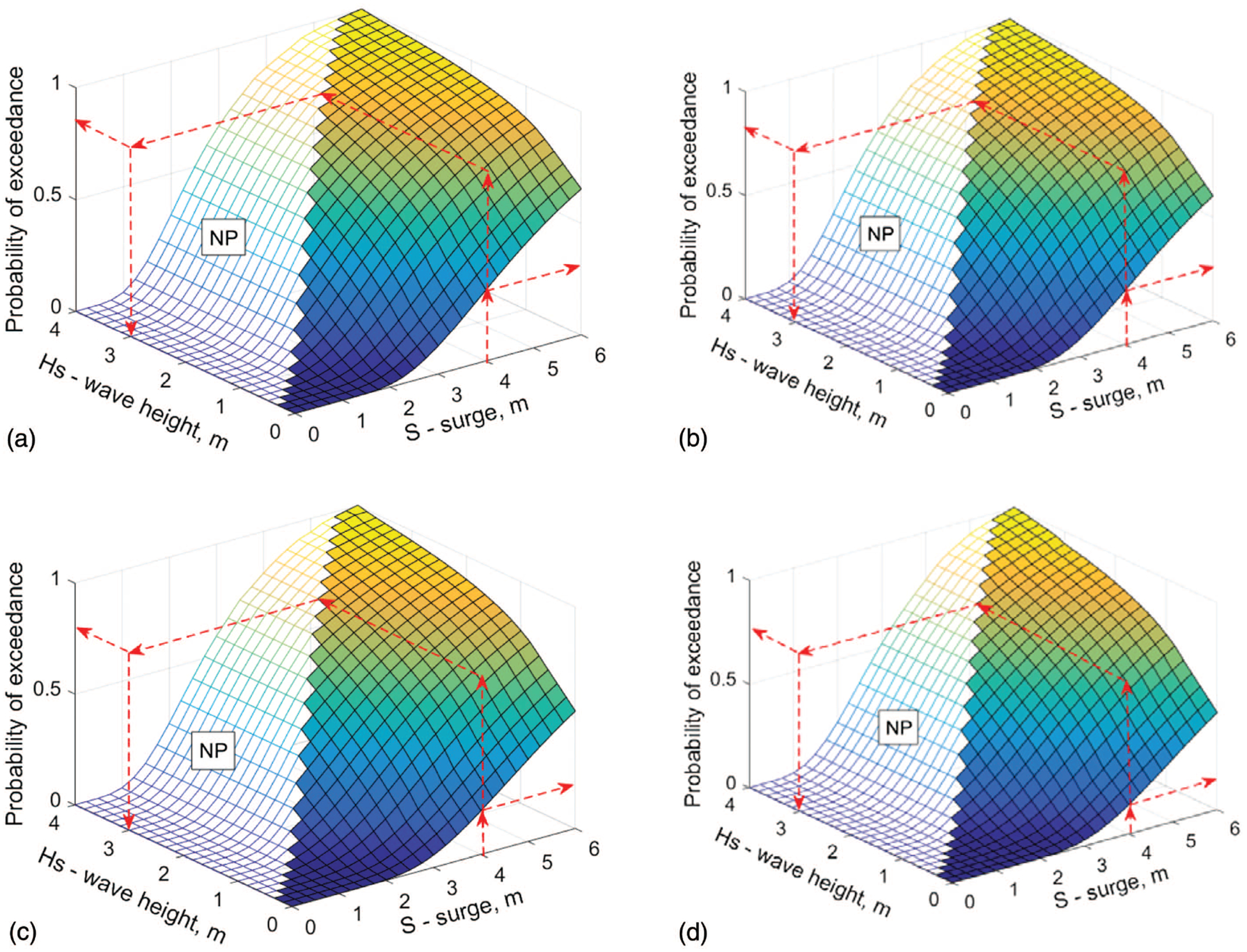
(Color) Fragility surfaces for components’ damage of 3-m elevated building. NP = not possible combination of H_s − S: (a) DS1; (b) DS2; (c) DS3; and (d) DS4.

For the slab-on-grade building (Fig. 14), at a surge level of less than 1.0 m, there is almost no damage observed at the site with small waves. However, during a hurricane with maximum design wave height of 1.0 m for a surge level of 1.0 m, 60%, 50%, 45%, and 25% of the analyses exceed damage states 1, 2, 3, and 4, respectively. The building was completely in damage states 1 and 2 when surge levels reached 4.0 m for any wave condition as one might expect. However, at this surge level, damage state 3 probability increases from 45% to 90% [Fig. 14(b)], and damage state 4 probability increases from 30% to 80% [Fig. 14(d)], with the increase of significant wave height from 0 to 1 m. It is also interesting to note from Fig. 14(d) that, for the site with surge only (Hs = 0 m), the slab-on-grade building experiences a 50% chance of exceeding damage state 4 (structural damage) although the building is totally under water (surge level of 6 m). This is typical for a non- or low-velocity flood because it does not directly damage the structure.

If the building was raised 3 m from the ground as discussed previously, the resulting fragilities for different damage states are shown in Fig. 15. At a surge of 4 m and comparing results to the slab-on-grade building, without wave effects, there is a 30%, 25%, 20%, and 15% probability of the building exceeding damage states 1, 2, 3, and 4, respectively. However, the probabilities of exceeding damage states 1 and 2 increase to 80%, and probabilities of exceeding damage states 3 and 4 increase to 75% at a significant wave height of 3.0 m and surge level of 4 m.

Fragility curves for different surge levels are shown in Fig. 16 in 2D. At a surge level of 1.0 m [Fig. 16(a)], the significant wave height varies from 0 to 1.0 m. For the slab-on-grade building, when the significant wave height reaches 1.0 m, the building has a 60%, 50%, 43%, and 22% probability of exceeding damage states 1, 2, 3, and 4, respectively. On the other hand, at the same water level above the first floor, i.e., a surge level of 4.0 m for the 3-m elevated building in Fig. 16(b), the significant wave height can be up to 3.0 m. At the same water level above the first floor and a significant wave height of 1.0 m, the 3-m elevated building [Fig. 16(b)] has a 60%, 57%, 49%, and 41% probability of exceeding damage states 1, 2, 3, and 4, respectively. This is because at higher surge levels, higher waves can develop that obviously result in much higher forces on the building components and more damage to the building. These are expected trends, but the fragilities developed in this study will specifically allow detailed quantification of the relationship between surge, wave height, and the probability of resulting damage. In particular, calibration with DHS-FEMA field study data will allow the fragilities within HAZUS to account for wave forces for near coast buildings with better accuracy than when flood (i.e., surge) depth alone is used.

Fig. 16.

(Color) Fragility curve for some specific surge levels: (a) “slab-on-grade,” surge = 1 m; and (b) “3-m elevated,” surge = 4 m.

In addition, Fig. 17 shows the effect of surge levels on fragilities for both slab-on-grade and 3-m elevated buildings with different wave heights. With 0 m significant wave height or flood only [Fig. 17(a)] DS1 has a 50% chance of occurring at 1.7 m of surge for the slab-on-grade building and at 5.0 m of surge for the 3-m elevated building. However, at a significant wave height of 1.0 m for the 3-m elevated building, the probability of DS1 occurring is 50% at a surge level of 3.4 m [Fig. 17(b)].

Fig. 17.

(Color) Fragility curve for some specific significant wave heights: (a) significant wave height, Hs = 0 m; and (b) significant wave height, Hs = 1 m.

Finally, the total loss as a function of surge level was computed by summing the component losses and is presented in Fig. 18 for different wave conditions in which the surge level is relative to the first floor for a slab-on-grade building. Note that significant wave height of 1.0 m appears at a surge level of 1.0 m and higher; and significant wave height of 2.0 m starts at a surge level of 2.5 m based on physics of waves. From Fig. 18, one can see the inclusion of waves on the percent damage becomes noticeable when increasing the surge level from 0 to 2.0 m. At a surge level of 2.0 m, the total economic loss in the case without the wave effect (flood only) is about 60% but increases to almost 80% with a significant wave height of 1.0 m.

Fig. 18.

(Color) Comparison of total loss to FEMA cost damage estimator for a single-family dwelling at coastal V-zone, no obstruction.

The loss curves were also compared to the FEMA cost damage estimator curve for a single family one-story building in coastal V_zone, no obstruction (Tomiczek et al. 2014). The loss curves match well with the FEMA curve for the small wave effect (wave height is less than 0.5 m), but then begins to deviate, as they should, for larger wave heights.

Summary and Conclusions

In this study, a methodology was presented that generates fragility surfaces for near-coast structures subjected to combined waves and surge with the consideration of damage to building components such as windows, doors, walls, and floors. In order to consider all building components at the same time, two building archetypes of single family dewellings representative of slab-on-grade and an elevated building in coastal zones were modeled at full-scale in 3D using the Volume of Fluid model in ANSYS-Fluent. In this model, the buildings were considered as the fixed internal boundary walls of the fluid volume around the building as a numerial wave flume. The TMA wave spectrum was set as the boundary condition for one end of the numerical wave flume to generate the expected wave height at a series of existing water levels to create an array of possible wave and surge conditions at the building location. A 5-min hurricane duration was simulated for each wave and surge combination, and the distibution of maximum pressure on building components was obtained simultaneously. To obtain the distribution of maximum pressures on building components in a longer hurricane duration, a projected method was proposed under an assumption that the distribution types for maximum pressures remain the same for the longer hurricane duration. The developed fragility formulation using Monte-Carlo simulation was then applied to obtain the fragility surface for both slab-on-grade and elevated buildings subjected to hurricane wave and surge.

In addition, a prescribed amount of uncertainty can be added to the fragility calculation using the methodology described in this paper. This amount of uncertainty can be calibrated based on DHS-FEMA (or other) field study data on damage and loss. These fragilities can then be used within the current HAZUS-MH model for loss analysis that would provide a mechanism for HAZUS-MH to include the effect of waves in loss calculations.

However, the loss analysis in this study was based only on the fragilities of exterior components such as windows, doors, walls, and floors. Better estimates of content loss and interior components would further improve the model. The methodology presented herein is extensible to other building types, but was illustrated on a wood residential building since they are most prone to structure damage from waves and surge in near-coast situations.

In order to implement this work into damage, loss, and resilience analysis, other fragilities must be developed for other building archetypes in a coastal community using this methodology. Once the modeling results for a suite of coastal structures is obtained, transfer functions to obtain the wave loadings on elevated structures from a given random wave spectrum can likely be developed.

On the other hand, the uncertainty of the fragility model must be further investigated. These uncertainties are dependent not only on the modeling process but also the quality of the wave record, modeling, and the design requirements.

Notation.

The following symbols are used in this paper:

• H_s (m) = significant wave height, which is the average of 1/3 of the highest wave;

• S(m) = surge level or the still water or flood level from the ground;

• T_p(s) = peak period of wave;

• β_a = added uncertainty to a fragility curve;

• β₀ = calculated uncertainty of a fragility curve;

• β_tol = total uncertainty of a fragility curve; and ρ (kg=m³) = density (sea water or air).

References

- Amini MO, and van de Lindt JW. 2014. “Quantitative insight into rational tornado design wind speeds for residential wood-frame structures using fragility approach.” J. Struct. Eng 140 (7): 1–15. 10.1061/(ASCE)ST.1943-541X.0000914. [DOI] [Google Scholar]
- Ang AH-S, and Tang WH. 2007. Probability concepts in engineering Hoboken, NJ: Wiley. [Google Scholar]
- ANSYS. 2009. ANSYS fluent theory guide Canonsburg, PA: ANSYS. [Google Scholar]
- Blake ES, Kimberlain TB, Berg RJ, Cangialosi JP, and Beven II JL. 2013. Tropical cyclone report Hurricane Sandy (AL182012) 22–29 October 2012 Miami: National Weather Service, National Hurricane Center. [Google Scholar]
- Bradner C, Schumacher T, Cox D, and Higgins C. 2011. “Experimental setup for a large-scale bridge superstructure model subjected to waves.” J. Waterway, Port, Coastal, Ocean Eng 137 (3): 3–11. 10.1061/(ASCE)WW.1943-5460.0000059. [DOI] [Google Scholar]
- Bradner C, Schumacher T, Cox DT, and Higgins C. 2008. “Large-scale laboratory measurements of wave forces on highway bridge superstructures.” In Proc., 31st Int. Conf. on Coastal Engineering, 3554–3566. Reston, VA: ASCE. [Google Scholar]
- Bulleit WM, Pang W, and Rosowsky DV. 2005. “Modeling wood walls subjected to combined transverse and axial loads.” J. Struct. Eng 131 (May): 781–793. 10.1061/(ASCE)0733-9445(2005)131:5(781). [DOI] [Google Scholar]
- Do TQ, van de Lindt JW, and Cox DT. 2016. “Performance-based design methodology for inundated elevated coastal structures subjected to wave load.” Eng. Struct 117 (15): 250–262. 10.1016/j.engstruct.2016.02.046. [DOI] [Google Scholar]
- FEMA. 2009. Multi-hazard loss estimation methodology: Hurricane model HAZUS-MH-MR4. Washington, DC: FEMA. [Google Scholar]
- FEMA. 2015. Multi-hazard loss estimation methodology; Flood model; Hazus-MH flood model technical manual Washington, DC: FEMA. [Google Scholar]
- FEMA. 2017. Hazus tsunami model technical guidance Washington, DC: FEMA. [Google Scholar]
- Gromala DS 1983. Light-frame wall systems: Performance and predictability USDA Research Paper FPL 442. Madison, WI: Forest Products Laboratory. [Google Scholar]
- Gurley K, Pinelli JP, Subramanian C, Cope A, Zhang L, and Murphree J. 2005. Predicting the vulnerability of typical residential buildings to hurricane damage, Florida public hurricane loss projection model (FPHLPM) engineering team final report Miami: I.H.R. Center, Florida International Univ. [Google Scholar]
- Hasselmann K, et al. 1973. Measurements of wind-wave growth and swell decay during the joint north sea wave project (JONSWAP) Hamburg, Germany: Deutsches Hydrographisches Institut. [Google Scholar]
- Hughes SA 1984. The TMA shallow-water spectrum description and applications Technical Rep. No. CERC-84–7, Vicksburg, MS: USACE. [Google Scholar]
- Kennedy A, Rogers S, Sallenger A, Gravois U, Zachry B, Dosa M, and Zarama F. 2011. “Building destruction from waves and surge on the Bolivar Peninsula during Hurricane Ike.” J. Waterway, Port, Coastal, Ocean Eng 137 (3): 132–141. 10.1061/(ASCE)WW.1943-5460.0000061. [DOI] [Google Scholar]
- Knabb RD, Rhome JR, and Brown DP. 2006. “Tropical cyclone report: Hurricane Katrina Miami: National Hurricane Center. [Google Scholar]
- Kwon O-S, Kim E, and Orton S. 2011. “Calibration of live-load factor in LRFD bridge design specifications based on state-specific traffic environments.” J. Bridge Eng 16 (Dec): 812–819. 10.1061/(ASCE)BE.1943-5592.0000209. [DOI] [Google Scholar]
- Linton D, Gupta R, Cox D, and van de Lindt J. 2015. “Load distribution in light-frame wood buildings under experimentally simulated tsunami loads.” J. Perform. Constr. Facil 29 (1): 04014030. 10.1061/(ASCE)CF.1943-5509.0000487. [DOI] [Google Scholar]
- Linton D, Gupta R, Cox D, van de Lindt J, Oshnack ME, and Clauson M. 2013. “Evaluation of tsunami loads on wood-frame walls at full scale.” J. Struct. Eng 139 (8): 1318–1325. 10.1061/(ASCE)ST.1943-541X.0000644. [DOI] [Google Scholar]
- NOAA (National Oceanic and Atmospheric Administration). 2006. “Reports from the national data buoy center’s stations in the Gulf of Mexico during the passage of Hurricane Katrina” Accessed July 11, 2017. http://www.ndbc.noaa.gov/hurricanes/2005/katrina/.
- NOAA (National Oceanic and Atmospheric Administration). 2017. “Wave heights: Hurricane Sandy 2012” Accessed March 26, 2019. https://sos.noaa.gov/datasets/wave-heights-hurricane-sandy-2012/.
- Padgett JE, Spiller A, and Arnold C. 2012. “Statistical analysis of coastal bridge vulnerability based on empirical evidence from Hurricane Katrina.” Struct. Infrastruct. Eng 8 (6): 595–605. 10.1080/15732470902855343. [DOI] [Google Scholar]
- Park H, Do T, Tomiczek T, Cox DT, and van de Lindt JW. 2018. “Numerical modeling of non-breaking, impulsive breaking, and broken wave interaction with elevated coastal structures: Laboratory validation and inter-model comparisons.” Ocean Eng 158 (Jan): 78–98. 10.1016/j.oceaneng.2018.03.088. [DOI] [Google Scholar]
- Park H, Tomiczek TJ, Cox DT, van de Lindt JW, and Lomonaco P. 2017. “Experimental modeling of horizontal and vertical wave forces on an elevated coastal structure.” Coastal Eng 128: 58–74. 10.1016/j.coastaleng.2017.08.001. [DOI] [PMC free article] [PubMed] [Google Scholar]
- SWAN (Simulate Waves Nearshore). 2017. “User manual SWAN Cycle III version 41.20” Accessed July 11, 2017. http://swanmodel.sourceforge.net/download/zip/swanuse.pdf.
- Tomiczek T, Kennedy A, and Rogers S. 2014. “Collapse limit state fragilities of wood-framed residences from storm surge and waves during Hurricane Ike.” J. Waterway, Port, Coastal, Ocean Eng 140 (1): 43–55. 10.1061/(ASCE)WW.1943-5460.0000212. [DOI] [Google Scholar]
- van de Lindt JW, and Fu G. 2002. Investigation of the adequacy of current bridge design loads in the State of Michigan Lansing, MI: Michigan Dept. of Transportation. [Google Scholar]
- van de Lindt J, Gupta R, Cox DT, and Wilson J. 2009. “Wave impact study on a residential building.” J. Disaster Res 4 (6): 419–426. [Google Scholar]
- Winterstein SR, Jha AK, and Kumar S. 1999. “Reliability of floating structures: Extreme response and load factor design.” J. Waterway, Port, Coastal, Ocean Eng 125 (Aug): 163–169. 10.1061/(ASCE)0733-950X(1999)125:4(163). [DOI] [Google Scholar]