In-Depth Quantification of Cell Division and Elongation Dynamics at the Tip of Growing Arabidopsis Roots Using 4D Microscopy, AI-Assisted Image Processing and Data Sonification

Abstract

One of the fundamental questions in plant developmental biology is how cell proliferation and cell expansion coordinately determine organ growth and morphology. An amenable system to address this question is the Arabidopsis root tip, where cell proliferation and elongation occur in spatially separated domains, and cell morphologies can easily be observed using a confocal microscope. While past studies revealed numerous elements of root growth regulation including gene regulatory networks, hormone transport and signaling, cell mechanics and environmental perception, how cells divide and elongate under possible constraints from cell lineages and neighboring cell files has not been analyzed quantitatively. This is mainly due to the technical difficulties in capturing cell division and elongation dynamics at the tip of growing roots, as well as an extremely labor-intensive task of tracing the lineages of frequently dividing cells. Here, we developed a motion-tracking confocal microscope and an Artificial Intelligence (AI)-assisted image-processing pipeline that enables semi-automated quantification of cell division and elongation dynamics at the tip of vertically growing Arabidopsis roots. We also implemented a data sonification tool that facilitates human recognition of cell division synchrony. Using these tools, we revealed previously unnoted lineage-constrained dynamics of cell division and elongation, and their contribution to the root zonation boundaries.

Introduction

A striking feature of plant development is the post-embryonic formation of new organs and their indeterminate growth. Plants also exhibit a high degree of developmental plasticity whereby growth rate and final morphologies can vary with external cues. Because plant organ growth is determined by oriented cell division and anisotropic cell expansion, quantitative analyses of cell division and elongation dynamics are critical to understanding the mechanisms regulating both stationary growth and their modification to adapt to fluctuating environments. An amenable model system to study cell division and elongation dynamics in plants is the tip of Arabidopsis thaliana (hereafter called Arabidopsis) roots (Fig. 1). Due to its high transparency and stereotypical tissue patterning (Fig. 1B), the Arabidopsis root tip has been widely used as a model system in plant cell and developmental biology and made a great contribution to constructing principles in plant development (Petricka et al. 2012, Motte et al. 2019).

Fig. 1.

The cellular organization of the Arabidopsis root tip and fluorescent labeling of cortex nuclei for live imaging. (A) The longitudinal optical section of the Arabidopsis root tip. RAM is composed of the PD and the TD. PD and TD are largely synonymous to the MZ and the TZ, respectively, in other naming (Ivanov and Dubrovsky 2013). The EZ and the DZ (out of the section) are located proximal to the RAM. (B) The illustration of the cell arrangement in the RAM. At the distal end of the PD, QC and surrounding initial cells constitute the SCN (magnified in B’). In young Arabidopsis roots, the cortex cell layer is composed of eight cell files (orange). Cortex cells are derived from the cortex/endodermis initial (CEI) cells (green) adjacent to the QC (purple) in the SCN. MDCCs defined in this study are shown in magenta. (C, D) The longitudinal medial cross-section (C) and maximum intensity projection (D) showing CO2pro:tdTomato-nls expression (fire colors) and cell walls (white). (C’) and (C’’) are magnification of the box regions in (C). (D’) is a cross-section reconstructed from the region indicated in (D). CO2 promoter is active almost exclusively in the cortex layer, not in QC and CEI. tdTomato-nls is localized to the nuclei in non-dividing cells (C’, blue arrowheads), whereas diffusing in the cytoplasm in dividing cells (C’, yellow arrowhead). In (A), (C) and (D), cell walls were stained with SR2200. Scale bar, 200 µm (A), 100 µm (C, D); 25 µm (C’, C’’); 50 µm (D’).

In the root of most flowering plants including Arabidopsis, domains of cell proliferation, elongation and differentiation are spatially separated along the proximodistal axis (Ivanov and Dubrovsky 2013) (Fig. 1A). At the distal end of the proliferation domain (PD), mitotically dormant quiescent center (QC) cells and their surrounding stem cells (called ‘initials’) constitute the stem cell niche (SCN). Daughter cells produced by the formative division of the initials subsequently undergo proliferative divisions (sometimes called rapid amplification) in the proximal domain and eventually exit from the mitotic state to start slow elongation. In the further proximal region, cells undergo rapid longitudinal elongation before starting morphological and functional specialization. Based on these cellular behaviors, the Arabidopsis root tip was classically divided into three zones: the meristematic zone (MZ), the elongation zone (EZ) and the differentiation zone (DZ) along the root longitudinal axis (Dolan et al. 1993, Ivanov and Dubrovsky 2013). More recently, the existence of the transition zone (TZ) between the MZ and the EZ has been acknowledged although there has been a confusion in both the definition and terminology of the TZ (Baluska et al. 2010, Ivanov and Dubrovsky 2013, Salvi et al. 2020a). The TZ is generally regarded as a region where cells lost (or losing) proliferative capacity, yet do not initiate rapid cell elongation. Due to this ambiguous definition of the TZ, especially for the existence of remaining proliferative activities, a new nomenclature has been proposed, where the TZ and the MZ are together called the root apical meristem (RAM), which is separated into the distal proliferation domain (PD) and the proximal transition domain (TD) (Fig. 1A). Because both the timing and the positions of cell elongation initiation are critical to determining root growth control and tropic responses, many physiological roles have been implicated in the TZ (Baluska et al. 2010, Kong et al. 2018, Wang et al. 2023).

Positions of the root zonation boundaries have been conventionally inferred based on the size distribution patterns of cortex cells whereby a region filled with equally small cells is considered the MZ (or the PD). MZ size has been measured by direct observation of mitotic figures after the incorporation of fluorescent dyes or nucleotide analogs (Schmidt et al. 2014, Lavrekha et al. 2017, Pasternak et al. 2022) and by using G2/M phase reporter lines such as CycB1;1-GUS and CycB1;1-GFP (Colón-Carmona et al. 1999, Pacheco-Escobedo et al. 2016, Lavrekha et al. 2017). Upon exit from the mitotic state, cells continue slow elongation to form a cluster of slightly enlarged cells, a hallmark of the TZ (or the TD). In some plant species, however, cell division occurs in the TD defined by cell size (Ivanov and Dubrovsky 2013). Furthermore, positions of the PD/TD boundary can vary with time and even within a single root tip (van den Berg et al. 2021). Thus, in order to precisely define the zonation boundaries (if possible), it is essential to observe cell division and elongation dynamics by time-lapse imaging and extract quantitative parameters from the 4D image data.

While the technique of cell-level time-lapse imaging has been available for the Arabidopsis shoot apical meristem for nearly two decades (Heisler et al. 2005), its application to the root meristem had been difficult because the root tip is readily displaced from the microscopic observation field by the root growth. To overcome this problem, motion-tracking microscopes have been developed by some research groups (von Wangenheim et al. 2017, Rahni and Birnbaum 2019). By using this technique, Rahni and Birnbaum (2019) revealed largely constant cell division intervals (16–25 h) of rapidly amplifying cells of various root tissues. In another research group, von Wageningen et al. constructed a motion-tracking microscope with a horizontal light axis allowing naturally downward root growth. Using this microscope and a plant line that ubiquitously expressed plasma membrane–localized yellow fluorescent protein (YFP), they presented time-resolved cell amplification and cell elongation images for a single cortex cell file (von Wangenheim et al. 2017). These previous studies, however, did not dissect the cell division and elongation dynamics in the context of cell lineages nor the synchrony across cell files, likely due to the difficulty of capturing all cell files in a single root. Moreover, while motion-tracking microscope systems have been proven useful in capturing 4D images of the root tip, annotating all cells and tracing their lineages is an extremely labor-intensive and time-consuming task for human researchers. Thus, new techniques to automate image-processing tasks are crucial to achieve a breakthrough in the root developmental biology.

Image segmentation has become a conventional tool in many research fields, especially in medical image analysis where target organs or lesions are segmented out from other tissues in diagnostic images. In plant developmental biology, cell segmentation has been utilized to extract cell outlines from the microscopic images to analyze their positions and morphologies in the tissues (Barbier de Reuille et al. 2015). Recent advances in the deep learning–based methods greatly improved the prediction accuracy and expanded the range of its application to basic research. Networks like Fully Convolutional Network (FCN) (Long et al. 2015), U-Net (Ronneberger et al. 2015), U-Net++ (Zhou et al. 2018), U-Net3+ (Huang et al. 2020) and DeepLab (Chen et al. 2017, 2018) series are commonly used in various tasks.

In this study, we established a 4D-microscope system and an image-processing pipeline that can semi-automatically quantify cell division and elongation dynamics of the cortex cell files at the tip of growing Arabidopsis roots. This is achieved by developing (i) a motion-tracking spinning disc confocal microscope with a horizontal optical axis, (ii) a deep learning- and genetic algorithm (GA)-assisted image-processing pipeline and (iii) data presentation tools to assist interpretation by human researchers. By using these tools, we uncovered lineage-associated constraints in the cell division and elongation dynamics and their contribution to the root developmental boundaries.

Results

Establishment of a time-lapse confocal imaging system for the tip of growing roots

To capture cellular and subcellular dynamics in the tip of growing Arabidopsis roots as a 4D (3D-space plus time) image data, we established a microscope system that automatically tracks the tip of growing roots for several days. For this, an inverted microscope (Nikon ECLIPSE Ti2-E) was mounted to a custom-made steel support on a vibration-isolation table in a laid-down orientation (Fig. 2A). This configuration allowed the sample stage to orient vertically, thereby ensuring the roots to grow naturally downward (Figs. 2B, C). For the fluorescence imaging and root-tip tracking, a spinning disc confocal unit (Yokogawa CSU W1) and a sCMOS camera (Hamamatsu ORCA-Fusion) were attached to the bottom port of the microscope. To physically track the root tip, a motorized microscope stage was installed and controlled by the ‘Keep Object in View’ plug-in of the Nikon NIS-elements software. This commercial software recognizes the object shape in contrasted bright-field images to automatically shift the stage to compensate for the sample relocation (Figs. 2D, E). A line-shaped light-emitting diode (LED) unit was mounted above the microscope stage and controlled by the NIS-elements software to synchronize with fluorescent image capturing (Fig. 2A). The overall design is similar to the previously reported system by another group (von Wangenheim et al. 2017), except that our system adopted the spinning disc confocal unit to reduce photo damaging and the commercially available software.

Fig. 2.

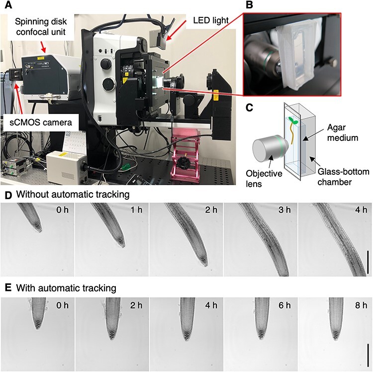
The long-term time-lapse imaging of the tip of growing Arabidopsis roots using a motion-tracking microscope with a horizontal optical axis. (A–C) Configuration of the motion-tracking microscope with horizontal optical axis. An inverted microscope (Nikon ECLIPSE Ti2-E) was fixed in a laid-down orientation to a steel support and attached with a spinning disc confocal unit (Yokogawa CSU W1) and a sCMOS camera (Hamamatsu Photonics ORCA-Fusion) through a bottom port (A). To achieve both plant growth and fluorescence imaging, a line-type LED unit was mounted on top of the microscope stage and controlled by the Nikon NIS-element software. Plants were allowed to grow in a sterile chamber with their roots elongating between the cover glass bottom and a block of agar medium (B, C). (D, E) Representative capture images of time-lapse imaging. Without motion-tracking, the root tip moved out of the frame in a few hours (D). With automatic object tracking using the ‘Keep object in view’ plug-in (Nikon), the root tip remained in the same position during several days of observation (E). Scale bar, 200 µm.

For long-term time-lapse imaging, 3-d-old seedlings were placed at the bottom of a chambered coverslip with their roots covered by a block of agar medium (Figs. 2B, C) and allowed to grow at an ambient temperature (approximately 22°C) on the microscope stage. Plants were continuously illuminated except for the time of fluorescence image capturing (typically 40 s for taking 29 stack images) to observe stationary root growth without the influence of light/dark cycles. To ensure precise root-tip tracking and cell imaging with minimal photo damaging, 2D bright-field images were taken in short intervals (5 min) for tracking, whereas fluorescent z-stack images were captured in sparse (30 min) intervals. The relevance of the 30-min interval for capturing nucleus division is confirmed by separately checking the division dynamics captured at 15-min intervals, where all division events examined were found to take >30 min (n = 138) at least for the cortex cell files. With this setup, we could successfully visualize the cell dynamics in the tip of growing roots for up to 5 d.

4D imaging of root cortical cell nuclei

Using our microscope system, we aimed to quantify cell division and elongation dynamics in the tip of growing Arabidopsis roots. Among the radially arranged root tissues, we visualized the cortex that is a single-layered tissue composed of eight cell files (Fig. 1B). In Arabidopsis, cortical cells exhibit relatively uniform shapes and are thus conventionally used to define the root zonation (Fig. 1A) (Salvi et al. 2020a). We established a fluorescent marker line that expresses nuclear-localized red fluorescent protein (RFP) reporter by a cortex-specific CO2 promoter (Heidstra et al. 2004) (CO2pro:tdTomato-nls). We opted for nuclear-localized free tdTomato in this work, rather than those utilizing chromatin proteins such as histones, to minimize the potential detrimental effects of nucleosomal fluorescent reporters on cell division dynamics. The bright red fluorescent signal of nuclear-localized tdTomato-nls visualized nuclear dynamics in all eight cortex cell files using the confocal optics (Figs. 1C, D). We could easily distinguish dividing and non-dividing nuclei based on the characteristic shape of fluorescent images: a round and focused image for non-dividing nuclei and a dispersed image for dividing nuclei (Fig. 1C’’, Supplementary Movie 1). In addition to the cell division dynamics, longitudinal cell length (subsequently called cell size) could be measured using the distance to the flanking nuclei in the same cell file, owing to the centrally localized nuclei in each cell (Figs. 1C, D). With the establishment of a microscope system and fluorescent marker line, we next developed an image-processing pipeline that enables automatic detection of dividing and non-dividing nuclei and their lineage tracking from the 4D image data.

Deep learning- and GA-assisted detection and tracking of nuclei in 4D images

The 4D image data captured by our microscope with a x20 objective lens typically contained >300 nuclei per time point (∼40 nuclei per cell file). They frequently divided and dynamically moved in the image volumes due to cell elongation and root twisting, leaving their quantitative annotation and lineage tracing far beyond the capacity of humans. To automate this task, we initially tested the publicly available TrackMate plug-in of ImageJ (Tinevez et al. 2017, Ershov et al. 2022), which features a user-friendly interface to perform tracking, data visualization and manual editing. We however became aware that the detection and particle-linking algorithms of TrackMate were not suitable for our 4D image data that contained densely localized and simultaneously dividing nuclei with variable fluorescent intensities. Accordingly, we developed our own image-processing pipeline suitable for our 4D images.

Our image-processing pipeline is composed of several modules as outlined in Fig. 3. The first module is a deep learning–based detection of dividing and non-dividing nuclei (Fig. 3A). In this module, we adopted a 2D slice-by-slice segmentation method to accurately detect the dividing and non-dividing nuclei using the U-Net architecture (Supplementary Fig. 1). The U-Net is an encoder-/decoder-based network with skip connection (Ronneberger et al. 2015). The encoder extracts high-dimensional features and aggregates them at multiple levels, from which the decoder generates a semantic segmentation mask. The skip connection combines low-level feature maps with high-level semantic features and thereby enhances the segmentation performance (Ronneberger et al. 2015). For training and validation of nuclei detection, we prepared two 4D image datasets of 144 and 100 time point volumes each composed of 29 z-slices (2.5-µm intervals). We randomly selected 170 volumes (4,930 slices) as a training dataset, 24 volumes (696 slices) as a validation dataset and 50 volumes (1,450 slices) as a test dataset (here a ‘volume’ indicates a 3D data of one time point). All nuclei in the training datasets were manually labeled as either a dividing or a non-dividing nucleus by experienced biologists. We evaluated the prediction accuracy of our model using two parameters: ‘Precision’ (proportion of accurately predicted nuclei among all so-predicted nuclei) and ‘Recall’ (proportion of accurately predicted nuclei among all nuclei truly having that status). This evaluation indicated that non-dividing nuclei were predicted with high accuracy (‘Precision’, 86.0%; ‘Recall’, 99.0%), whereas dividing nuclei were predicted with lower accuracy (‘Precision’, 71.5%; ‘Recall’, 95.9%) (Supplementary Figs. 2G, H). The lower prediction accuracy of dividing nuclei is likely due to their diffuse fluorescent signals as compared with highly contrasted signals of non-dividing nuclei (Fig. 1C’’). Nuclei located closer to the objective lens could be detected with higher accuracy than those located away from the objective lens, likely due to weak fluorescent signals (Supplementary Figs. 2G, H). It was particularly difficult to distinguish two nuclei that were closely positioned along the z-axis. Nevertheless, our nuclei detection module achieved significantly higher accuracy than the detectors integrated into TrackMate [Laplacian of Gaussian (LoG) detector and CLIJ2 Voronoi Otsu Labeling] (Supplementary Fig. 2I). We manually corrected undetected or mis-annotated nuclei using spot editing tools of TrackMate with which our output data were made to be compatible (Tinevez et al. 2017, Ershov et al. 2022).

Fig. 3.

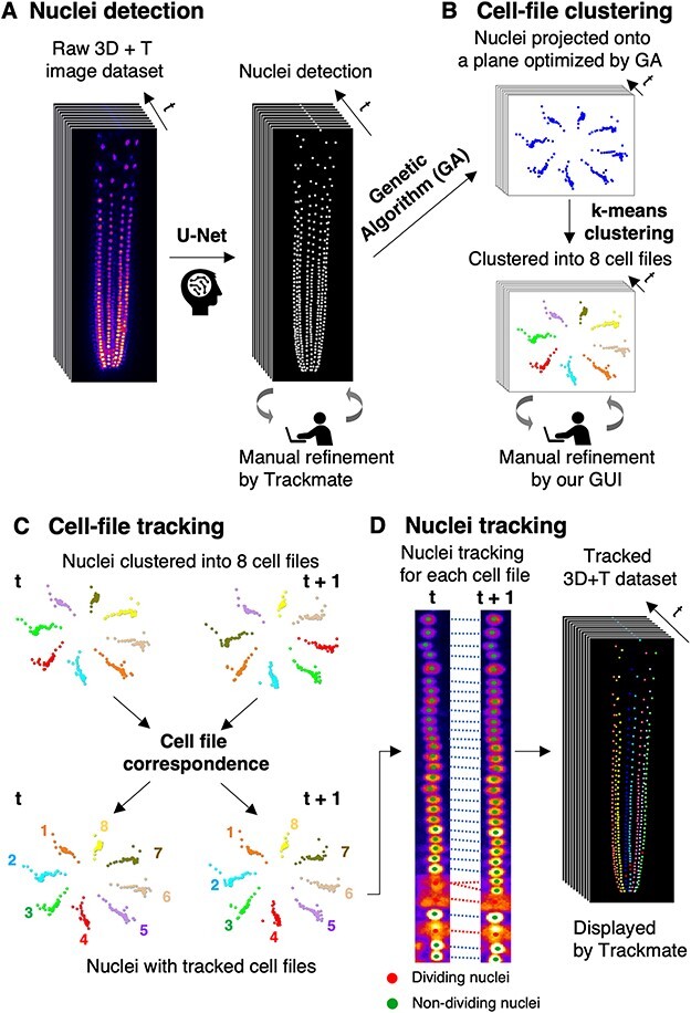
The outline of the AI-assisted semi-automatic nuclei detection and cell lineage-tracking system established in this study. (A) Nuclei detection. Dividing and non-dividing nuclei in a raw 4D image of CO2pro:tdTomato-nls plants were detected using a U-net-based deep-learning model. The remaining errors were manually corrected using the TrackMate plug-in on the Fiji platform (Tinevez et al. 2017, Ershov et al. 2022). (B) Cell-file clustering. For each time point, all annotated nuclei were projected onto an optimized plane determined by the GA to facilitate clustering of nuclei into eight groups by the k-means method. The remaining clustering errors were manually refined using the GUI established in this study. (C) Cell-file tracking. Clustered nuclei of two consecutive time points were correlated to each other based on positional information. (D) Nuclei tracking. Individual nuclei of each cell file were tracked across all time points in the whole dataset, incorporating division history.

After establishing the semi-automatic nuclei detection module, we developed the methods to allocate labeled nuclei to eight cell files (Fig. 3B), to correlate the cell files across time points (Fig. 3C) and to track the nuclei lineage within each cell file (Fig. 3D). Our initial attempt to utilize the conventionally implemented position-dependent nuclear tracking algorithm such as that adopted in TrackMate did not work with our image data that captured densely distributed and simultaneously dividing nuclei into continuously migrating cell files by root rotation. We therefore developed a novel tracking method by taking advantage of the clear geometrical arrangement of cortex nuclei and their limited anticlinal divisions in each cell file. To this end, all nuclei of each time frame were projected onto a plane whose orientation was optimized by a GA for k-means clustering of the nuclei into eight groups (Fig. 3B), and this method achieved a clustering accuracy of 99.5%. We also developed a graphical user interface (GUI) to facilitate manual correction of mis-annotated nuclei (Supplementary Fig. 3). Subsequently, cell files were tracked across adjacent time points (Fig. 3C), and individual nuclei and their lineages were tracked for each cell file by incorporating the information of division status (Fig. 3D). More detailed developmental procedure of this module will be published in a separate paper.

Graphical and audible presentation tools for data interpretation

We used the TrackMate program for initial assessment of cell division, cell elongation and cell trajectories, as well as for visual tracing of nuclei over time (Supplementary Fig. 4; Supplementary Movie 2) (Tinevez et al. 2017, Ershov et al. 2022). To perform a detailed quantitative analysis of cell dynamics, we developed a specialized program that automatically extracts nuclei locations from the data output and calculates the distance and displacement velocity between two neighboring nuclei, which correspond to cell–cell distance and cell elongation rate, respectively. Our program also generates kymographic representations for each cell file (Fig. 4A, 6A, Supplementary Figs. 5 and 6), as well as an animated presentation of cellular dynamics across all eight cell files (Supplementary Movie 3).

Fig. 4.

The distribution pattern of cell division frequency, timing and cell size along the root axis. (A) A kymographic plot of cell lineage traces in a single cell file. Segments connecting two consecutive divisions are colored according to the ordinal number of cell divisions. (B) The distribution pattern of the proportion of mitotic cells (MI). (C) The distribution pattern of cell size immediately before division (orange) and in other phases (gray). Cell size was estimated from the distance to the two adjacent nuclei. (D) A diagram explaining ‘division interval’ and ‘division time lag between sister cells’ shown in (E–G). (E) The distribution pattern of division intervals for all proliferating cells. (F) The distribution pattern of division intervals for distal (blue) and proximal (orange) sister cells produced by the previous division. (G) The distribution pattern of division time lag between the sister cells. Mean and SD values were plotted in 10-μm intervals. The number of events analyzed in Fig. 4 is listed in Supplementary Table 1.

Fig. 6.

The distribution patterns of cell size and cell elongation rate along the root axis. (A) Kymographic representation of cell lineages (dotted lines) and cell size (heat map) transition for a single cell file. (B) The distribution patterns of cell size (mean and SD) calculated in 10-μm intervals along the root axis. The number of analyzed events is listed in Supplementary Table 2. (C) The distribution pattern of the positions of final cell division in 10-μm intervals along the root axis relative to MDCC. (D) A plot showing the distribution patterns of the positions where the last two cell divisions occur for each cell in a single cortex cell file. Red and blue circles indicate the position of the last and the second last cell division for each cell (connected with a line). Segments are aligned in the order of the second last division. (E, F) The distribution patterns of cell size along the root axis plotted to the absolute distance from MDCC (E) and to the relative distance from the position of the final division (F). Line colors reflect the position of the final cell division for each cell. Sixty-five cell lineages from cell file #1 were analyzed. (G) The distribution patterns of the positions where cells larger than 15 μm (blue dots) and 35 μm (orange dots) first appeared during the time of observation.

Cell division in the MZ occurs simultaneously and at various locations, making it difficult to visually recognize their timing and positions. To further facilitate human recognition of cell division dynamics, we developed a human augmentation tool that presents cell division events in an audible manner. This visual-to-audio modality conversion technique is termed sonification (Grond and Berge 2011). To implement this technique, cell division events were assigned with musical notes of two different chord scales, C major and F# major, for two adjacent cell files. This chord selection is expected to facilitate the distinction of cell files as these scales are in a large harmonic distance in the circle of the fifth, a musical concept representing the relationship between different chords (Pilhofer and Day 2019, Laitz and Callahan 2023). Low to high tones were sequentially assigned to each division in a distal-to-proximal orientation along the root axis. The resulting soundtracks were superimposed on the visual presentation in which cell divisions were highlighted by color (Supplementary Movie 4). We realized that the sound facilitated human recognition of the position and timing of cell division events not only within a single cell file but also across the two cell files. By comparing with an additional soundtrack adopting only a single tone for each cell file (Supplementary Movie 5), we realized that the use of a series of low to high tones is effective in enhancing our recognition of cell division positions.

We also tested the feasibility of our sonification approach in facilitating the recognition of cell division synchrony across the cell files. To this end, we introduced random shifts to the data from a single cell file data (cell file #1) and sonificated it in parallel with the original data in F# major and C major chords, respectively (Supplementary Movie 6). As expected, the destruction of synchronicity could be easily recognized with increasing discrepancies (SD = 0 [0 min], 0.5 [15 min], 1 [30 min], 2 [60 min], 5 [150 min] and 10 [300 min] frames). By comparingly listening to this ‘synchrony scale’ and the original soundtrack of two adjacent cell files (Supplementary Movie 4), we could aware that cell divisions in the root cortex are out of sync across the cell files.

Cell division dynamics in the root cortex

Using the image-processing pipeline and data visualization tools established earlier, we analyzed cell division and elongation dynamics in the cortex layer of the growing Arabidopsis root. We used a dataset capturing about a 500-µm root tip region for 3 d, composed of 144 time volumes in 30-min intervals, and each consists of 29 z-slices in a 2.5-µm increment. After automatic nuclei segmentation, cell file and lineage-tracking and manual correction, a total of 51,410 spots (nuclear positions), 342 cell lineage tracks and 818 division events were annotated. Kymographic presentations and data quantification revealed four major features in the spatiotemporal dynamics of cell divisions in the root cortex (Figs. 4, 5 and Supplementary Figs. 5). First, cell divisions occur exclusively in the distal 200 µm region relative to the most distal cortex cell (MDCC) as previously evaluated using snapshot images (Pasternak et al. 2022). This region is hereafter called the RAM (Figs. 1, 4A and Supplementary Fig. 5). To further dissect the RAM, we plotted the proportion of cells undergoing mitosis [mitotic index (MI)] in 10-µm intervals (Fig. 4B). The plot revealed a middle subdomain in the RAM (30–160 µm relative to MDCC) that exhibits equally high MIs (3.7%). This MI value is comparable to that previously calculated from snapshot images (Pasternak et al. 2022). The middle subdomain is flanked by a distal (0–30 µm) or a proximal (160–200 µm) subdomain with reduced MI (2.1% and 0.7%, respectively). The quantification of cell division intervals (Figs. 4D, E) revealed that cells in the middle and the proximal subdomains divide in similarly short intervals (11.0 ±1.9 h and 11.6 ± 1.8 h, respectively), whereas those in the distal subdomain divide in significantly longer intervals (18.4 ± 7.3 h). Among the latter, MDCCs divide in the longest intervals (27.4 ± 8.9 h). Thus, our quantification revealed that cells in the distal subdomain divide less frequently but have similar mitotic potentials as the rapidly amplifying cells in the middle subdomain. By contrast, the proximal subdomain contains fewer mitotic cells (Fig. 4B), but their cell cycle progresses as rapidly as those in the middle subdomain (Fig. 4E).

Fig. 5.

The lack of cell division synchrony between adjacent cell files. (A) A diagram showing the definition of division time lags between adjacent cell files. For each reference division (α), time lags for the divisions in laterally abutting cells (μ) were extracted. (B) The proportions of cells with indicated division time lags (x-axis) are plotted. Note that the plots from our 4D image data (blue) and a simulation assuming no synchrony (orange) closely match each other. The simulation was carried out using cell division intervals randomly resampled from our 4D image data. Asynchronous status was induced by allowing 10,000 free divisions before the sampling starts.

The second feature is a largely constant cell size at the timing immediately preceding the division throughout the RAM (8.3 ± 0.9 µm, Fig. 4C). Nevertheless, cells in the proximal and the distal subdomains were slightly larger at division (9.4 ± 0.9 µm and 8.8 ± 1.0 µm, respectively) than those in the middle subdomain (8.2 ± 0.8 µm). Notably, cells in the distal subdomain exhibit strikingly longer cell division intervals but are nevertheless comparable in size before the division to the cells in the middle subdomain (Figs. 4C–E). The third feature is synchronized divisions of two sister cells derived from the previous division (Figs. 4D, F, G) although distal sister cells divide slightly but consistently earlier than proximal sister cells in the middle subdomain (−1.8 ± 2.7 h, 79.2%, n = 270). Interestingly, this order is reversed in the distal subdomain (+7.4 ± 12.5 h, 11.5%, n = 36) (Fig. 4G).

The fourth feature is the lack of cell division synchrony across the cell files. This feature could not be recognized easily in the visual representation (Supplementary Movie 3) but intuitively noticed by the asynchronous sound in the sonification tool (Supplementary Movie 4). To confirm this feature quantitatively, we carried out a mathematical simulation in which cells in three hypothetical cell files were allowed to divide in the intervals randomly sampled from the 4D image data. Division time lags between neighboring cell files were extracted from the simulation and the time-lapse image. Distribution patterns of the time lags showed a close overlap with no statistically significant difference (Fig. 5) (Kolmogorov–Smirnov test, K = 0.85, P = 0.46). Thus, our analysis confirmed the lack of cell division synchrony across the cortical cell files.

In summary, our image quantification revealed detailed cell division dynamics in the root cortex. Notably, the RAM is composed of three subdomains with distinct proportions of mitotic cells and division intervals. Nevertheless, most cells in the RAM divide at comparable sizes. Sister cells divide in a largely synchronous manner but with small and consistent lag time depending on cell position. By contrast, no signs of division synchrony were detected across the cell files.

Cell elongation dynamics and their contribution to root zonation boundaries

We next quantified spatiotemporal dynamics of cell size and cell elongation. As widely acknowledged, cells in the RAM (0–200 µm from MDCC) maintained small sizes (<10 µm), whereas those in the proximally flanked region (>200 µm from MDCC) enlarged progressively as they move away from the root tip (Figs. 6A, B, Supplementary Fig. 6). Interestingly, the kymographic plot visualized temporal fluctuation in the cell size distribution patterns, which appear to arise from periodically forming clusters of lineage-associated cells (striped patterns of light and dark blue colors in Fig. 6A). To quantitatively analyze these dynamics, we first plotted the positions of the final cell division along the root axis and found them to occur in the proximal 100-µm region in the RAM (Fig. 6C). Interestingly, file-by-file plots for each cell lineage further revealed that the regions accommodating the final division and the second final divisions barely overlap with each other (Fig. 6D, Supplementary Fig. 7, shaded in magenta and cyan, respectively). We next analyzed size trajectories following the final cell division and plotted them to either the absolute distance from MDCC or the relative distance from the position of the final cell division (Figs. 6E, F, Supplementary Fig. 8). These plots visualized comparable cell elongation behaviors after the final cell division regardless of their absolute positions in the RAM, indicating that the cell size is a simple readout of the displacement from the position at the final cell division. To visualize the spatiotemporal dynamics of cell size transition, we plotted the positions where cells of a certain threshold size become first detectable along the root axis. Interestingly, the plots visualized clear zigzag patterns for the cell size threshold of 15 µm, which corresponds to cells immediately after exiting the mitotic cycle (Fig. 6G, Supplementary Fig. 9, blue dots). Plots for the cell size threshold of 35 µm (correspond to the cells at the onset of rapid elongation) also exhibited zigzag patterns although diminished as compared to those for 15 µm (Fig. 6G, Supplementary Fig. 9, orange dots). These quantitative analyses support the notion that the fluctuating cell size distribution patterns arise from the synthetic interaction between temporal waves of final cell divisions, their occurrence in a relatively broad (∼100 µm) domain and similar elongation kinetics of cells exiting the mitotic state.

To correlate the abovementioned observations with previously proposed root developmental zones, we illustrated cell division and cell size transitions on a kymographic plot of cell lineage tracing (Fig. 7; the plot shown in Fig. 4A was used). In this cell file (#1), final cell division of each lineage occurred in the region spanning 90–200 µm relative to MDCC (red dots in Fig. 7). Because sister cells divide in a synchronous manner (Figs. 4F, G), the timings of final cell division tend to be largely synchronous across approximately eight lineage-sharing cells (clusters of red dots in Fig. 7). In the meanwhile, cells elongated similarly following the final division. These cellular behaviors together generate linear arrays of equally enlarged cells, which gradually protrude out of the RAM toward the proximal region (alternating production of cell arrays colored in blue and yellow in Fig. 7). Each cluster is flanked on its distal side by a newer cluster of smaller cells. Consequently, positions where slightly enlarged cells first appear (conventionally defined as the PD/TD boundary; thick red segments in Fig. 7) fluctuate over time. Although less conspicuous, positions where rapid cell elongation is first recognizable (conventionally defined as the TD/EZ boundary; thick blue segments in Fig. 7) also fluctuate over time. The size of the region occupied by slightly elongated cells (conventionally defined as the TD or the TZ) also fluctuates over time although the size of the TD itself is affected by the number of cells constituting each cluster.

Fig. 7.

A schematic diagram illustrating the process of temporally synchronized and spatially restricted final cell divisions generating the clusters of similarly sized cells. The scheme is overlayed on a kymographic plot of cell lineage tracing for the cell position (y-axis; distance from MDCC) and time (x-axis) for cell file #1. Small boxes and their vertical arrays indicated cells and cell clusters, respectively. Numbers in parentheses indicate the number of cells in each cluster at the time of exit from the mitotic cycle. Red dots indicate the final cell division of each lineage. Pink and green lines indicate the trajectories of the most proximal and the most distal cells of each cluster, respectively. Note that the sister cells of the second final divisions tend to segregate into different clusters. Linear arrays of similarly sized cells are produced in the RAM and translocated proximally. Note that the positions of the PD/TD boundary (thick red lines) and the TD/EZ boundary (thick blue line) apparently fluctuate over time by the influence of the cell clusters.

Discussion

Quantification of cellular dynamics at the tip of growing Arabidopsis roots by human–machine collaboration

Studies using the Arabidopsis root tip made a great contribution to establishing principles in plant development beyond root biology. This is owing to the unique structural features of the Arabidopsis root tip, such as radially symmetric tissue organization, spatially separated longitudinal zonation of cell division, cell elongation and cell differentiation and high tissue transparency suitable for microscopic observation. Radially symmetric tissue organization allows the use of a median longitudinal section to predict 3D morphology, whereas the exclusively basipetal progression of tissue patterning and cell differentiation allows the root longitudinal axis to serve as a pseudo-time axis. Accordingly, even 2D snapshot images have been effectively used to decipher 4D dynamics of cell differentiation and tissue patterning. While these advantages have been maximally utilized to elucidate developmental mechanisms, information regarding the exact behavior of individual cells and their variance in growing roots has been elusive due to the difficulty of tracking rapidly displacing root tips in the microscopic field. As a mean to overcome this problem, at least two research groups have previously constructed specialized microscopes with automatic root tip-tracking capacity (von Wangenheim et al. 2017, Rahni and Birnbaum 2019). Using this technique, Rahni and Birnbaum found that cells in the SCN, namely the initials and their daughter cells, exhibited exceptionally long cell cycle intervals as compared with proximally located cells (Rahni and Birnbaum 2019). This notion is confirmed in our study of cortex cell files although both root growth rate and cell cycle progression were about twice as faster than those reported previously likely due to our experimental setting allowing naturally downward root growth.

While motion-tracking microscopes are becoming a practical method, quantification of cell division and cell elongation dynamics from the captured 4D images is still a highly challenging task. To solve this problem, we established an image-processing pipeline consisting of machine learning–assisted segmentation of dividing and non-dividing nuclei and GA-based tracking of nucleus lineages in each cortex cell file. Currently, this technique is specialized for the Arabidopsis root cortex layer, which is composed of invariably eight files of relatively large cells and whereby widely used as a proxy to evaluate cell cycle and cell size control in root development. In our image-processing pipeline, the time required for automatic segmentation, cell-file clustering, cell-file tracking and nuclei tracking for a 4D image dataset (29 slices × 144 time points) is 30, 30, 3 and 10 min, respectively. As described earlier, however, our automatic annotation does not accomplish 100% accuracy as in any of such tools, and hence, it is necessary to manually correct the output data. While this manual correction typically takes 8 h for the whole 4D image, the use of our GUI and the TrackMate program allows a human to work on multiple 4D images in a practical time frame. As manually curated data accumulate, they can be used as training data to improve prediction accuracy, further strengthening the power of human–machine collaboration. In our hands, manual segmentation of all cortex nuclei of this 4D image would take 108 h, even if a researcher could keep working with constant efficiency and interest. While the nucleus annotation might be still within the reach of human capability, tracking all annotated nuclei and construction of the entire lineage maps are far beyond the capacity of ordinary humans like the authors of this paper. The insufficient fidelity of tracking using an Linear Assignment Problem (LAP) tracker implemented into TrackMate on our dataset is at least partially due to a large and simultaneous displacement of multiple nuclei between the frames via the rotation of the whole root tip. Our developed algorithm that takes into account the known spatial arrangement of cortical cell files and human–machine collaborative working is highly robust and reliable specifically for our dataset. Thus, our present study demonstrates the power of human–machine collaboration to solve fundamental problems in plant developmental biology.

In this study, we implemented a data sonification tool to assist human recognition of cell cycle synchronization. While sonification tools have been studied in the fields of practical sciences, their application in natural science is limited to our knowledge (Yu et al. 2019, Martin et al. 2021). In our study, the position of cell divisions, their synchrony within each cell file and their asynchrony across neighboring cell files could be easily recognized by ‘listening to’ the live-imaging data. While the efficacy of this technique is yet to be evaluated statistically with a sufficient number of monitors, data sonification has a potential to expand our capacity to recognize complex developmental phenomena in various biological systems.

Lineage-constrained cellular dynamics and their contribution to root developmental zonation

Our extensive quantification of the 4D image dataset revealed previously unnoted cellular behaviors at the tip of stationarily growing Arabidopsis roots. One interesting feature is the lineage-constrained cell division synchrony in each cortex cell file (Fig. 8). Daughter cells produced from the transverse division of MDCC (Fig. 8, purple box) subsequently divide five times to produce a linear array of ∼30 cells before leaving the RAM. Cell numbers in a lineage cluster do not reach 32 because 2–3 of the 16 daughter cells of the fourth division are pushed away from the RAM before the fifth division (Fig. 8). An exception to this division synchrony is the immediate daughter cells of MDCC, whose division intervals are considerably longer than other cells and staggered with each other. The extended and staggered division timings of these cells split the cell lineage into two blocks, with the cell cycle of the proximal block preceding that of the distal block by approximately one cell cycle length (green and orange clusters in Fig. 8). Additionally, we found that the domains where the last two divisions take place (fourth and fifth division) do not overlap with each other. These complex cell division procedures ultimately lead to the formation of two subclusters from a single MDCC daughter, each consisting of 16 or slightly fewer cells (Fig. 8). Because cells elongate in a similar kinetics after the exit from the mitotic cycle regardless of their absolute position, cells in each subcluster are similar in size. Due to the cell division synchrony, new subclusters are produced in a regular interval and push the preceding cluster away from the RAM. Consequently, positions of the apparent PD/TD border, as conventionally defined by the cell size distribution patterns, fluctuate over time (Fig. 7, 8). It should be noted that the cell division scheme shown in Fig. 8 is somewhat too simplified. In real roots, cell division intervals vary with a certain variance, and the division interval of the most distal cell is not exactly twice that of the proximal daughter cell. Consequently, the size of the subclusters can vary, as seen in the example shown in Fig. 7.

Fig. 8.

A simplified schematic presentation of the process generating subclusters of synchronously dividing cells. (A) The formation of synchronously dividing cell clusters. Division of an MDCC daughter (purple) divided further to generate two subclusters (green and orange). Due to the longer and lagged cell division intervals of the two daughter cells, the proliferation of the distal subcluster (orange) lags behind that of the proximal subcluster (green). Synchronized cell divisions and subsequent slow cell elongation result in the reiterated formation of the subclusters made of similarly sized cells. (B) Clusters of similarly sized cells can be recognized in a median snapshot image. Scale bar, 200 µm. The root image is a partial enlargement of the one shown in Fig. 1A.

Another interesting feature is asynchronous divisions across the neighboring cell files. This feature could be intuitively recognized from the asynchronous sounds in the data sonification tool and confirmed by comparing the distribution patterns of the division time lags between the live-imaging data and mathematical simulation assuming randomized divisions. While this asynchrony could have been noticed in the distribution patterns of mitotic cells in snapshot images (Lavrekha et al. 2017), our quantification of 4D live-image data and its statistical comparison with a mathematical simulation provided solid evidence for the asynchrony.

Future direction

Our image acquisition and data processing pipeline are currently optimized for the root cortex. Since previous studies indicated variable distribution patterns of mitotic cells in different tissue layers (Lavrekha et al. 2017, Pasternak et al. 2022), it is essential to extend our technique to other root tissues than the cortex. With the wealth of tissue-specific promoters available for the Arabidopsis root tip, the establishment of fluorescent maker lines should not be a problem. Screening of fluorescent markers suitable for neural network–based detection of cell cycle phases would also be effective. Image acquisition in deep optical sections, such as those containing epidermal cells away from the objective lens, is also practical with the use of bright fluorescent reporters. The greatest challenge would be lineage tracking of densely arranged and tangentially dividing cells such as those in the vascular cylinder, which likely requires de novo reconstruction of the tracking algorithm. We also realized the importance of the quantity and quality of training images in achieving optimal nuclei detection performance. Careful curation of training images for a given observation condition improves the robustness and adaptability of the nucleus detection tool.

With the availability of our semi-automatic image quantification pipeline, the next important step is to mechanistically link the cell-level dynamics to previously proposed models of gene regulation, hormone signaling and cell cycle regulation. For example, genetic pathways controlling the transition from the mitotic cycle to the endocycle have been extensively studied at multiple scales and hierarchies. Degradation of CYCA2;3 through inactivation of CDKB1;1, which in turn is regulated by CCS52A1, an activator of E3 ubiquitin ligase, anaphase-promoting complex/cyclosome (APC/C), plays an important role in the cell cycle transition downstream of cytokinin signaling (Boudolf et al. 2009, Takahashi et al. 2013). Our data revealed that the mitotic potential steeply decreases at the position 150 µm from MDCC. Given that the checkpoint for the cell cycle transition is in the G2-M phase (Inzé and De Veylder 2006), the true decision point should be somewhat closer to the root tip. According to the previous model, the CYCA2;3 degradation should occur at such positions. Antagonistic actions of the phytohormones auxin and cytokinin, mediated by mutual regulation between PLETHORA (PLT) and Type-B ARABIDOPSIS RESPONSE REGULATORs (B-ARRs), are known to serve as a global determinant of TD position (Dello Ioio et al. 2007, Ishida et al. 2010, Di Mambro et al. 2017, Salvi et al. 2020b, Shtin et al. 2023). It would be interesting to correlate the exact spatiotemporal dynamics of such antagonism with the cell-level behaviors in the root tip.

Finally, our image quantification revealed cluster-constrained cell size alternation in root cortex cells. Indeed, a recent computer simulation proposed a similar cellular behavior as a basis for the oscillating auxin response regulating the root branching patterns (van den Berg et al. 2021). Our live-imaging and data quantification tools are useful not only to extract realistic parameters for mathematical modeling but also to validate predicted models at cell resolution.

Materials and Methods

Generation and culture of CO2pro:tdTomato-nls plants

To prepare the CO2pro:tdTomato-nls reporter construct, a ∼610-bp promoter region of At1g62500 was amplified by PCR using the primers AD19_pCo2_Fw (5 ´–CTCTAGAGGATCCCCG ATCAGAGTATTGGGCCTTT–3 ´) and AD_tdToma_pCo2_rev (5 ´–C TTGCTCACCATCCCAACTCTTGTTGCATTATTGT–3 ´) and cloned into pAN19/tdTomato-nls_NOSt by the SLiCE reaction (Motohashi 2015). The resulting CO2pro:tdTomato-nls gene cassette was then transferred to pBIN41 (a binary vector derived from pBIN19 carrying a hygromycin-resistance gene) to give CO2pro:tdTomato-nls/pBIN41. This plasmid was introduced into A. thaliana accession Col-0 plants by the floral dip method using the Rhizobium tumefaciens strain C58MP90. Seedings were grown on vertically oriented Arabidopsis nutrient agar media (Okada and Shimura 1990) supplemented with 1% (w/v) sucrose and solidified with 1% (w/v) agar with the 16 h light/8 h regime at 23°C.

Tissue-clearing and confocal observation

Seven-day-old seedlings were fixed with 4% (w/v) paraformaldehyde for 30 min at room temperature, washed twice with a phosphate-buffered saline (PBS) and then cleared with the ClearSee solution, supplemented with 0.2% (v/v) SCRI Renaissance 2200 (Renaissance Chemicals, North Yorkshire, UK) for cell wall staining (Kurihara et al. 2015, Musielak et al. 2015). Images were captured using a Leica SP8 confocal microscope (Leica Microsystems, Wetzlar, Germany) with 405 nm and 552 nm laser for excitation of SR2200 and tdTomato, respectively.

Motion-tracking microscope with horizontal optical axis

An inverted microscope equipped with the Perfect Focus System (ECLIPSE Ti2-E, Nikon Solutions, Tokyo, Japan) was fixed on a custom-made steel support in a 90º tilted orientation to orient its sample stage vertically. A spinning disc confocal unit (CSU W1, Yokogawa, Tokyo, Japan) and a sCMOS camera (ORCA-Fusion, Hamamatsu Photonics, Shizuoka, Japan) were attached to the bottom port of the microscope. A motorized stage of Ti2-E was attached and controlled by the NIS-elements software (Nikon Solutions) with the ‘Keep object in view’ plug-in to automatically track the tip of growing roots. A custom-made stage attachment that can accommodate four chambers was attached to the sample stage to enable multi-point time-lapse imaging (typically two seedlings were grown in each chamber). To ensure plant growth during observation, sample chambers were continuously illuminated by a line-shaped LED light (LA-HDF108AA, HAYASHI-REPIC, Tokyo, Japan) except during the image acquisition. Tracking of the root tip, multi-point image acquisition and LED illumination were controlled by the Nikon NIS-elements platform integrated with Jobs plug-in (Nikon Solutions).

Three-day-old seedlings were transferred to a chamber slide (Lab-Tek chambered cover glass, Thermo Fisher Scientific, MA) and covered with a block of agar medium. Time-lapse imaging was performed with x20 objective lens (CFI Plan Apochromat Lambda D 20X, Nikon Solutions) with excitation by a 561 nm laser (50% attenuation by an ND filter, COHERENT, Pennsylvania, USA) and exposure time of 100 ms at ambient temperature (∼22–23°C). Image acquisition was typically started 1 d after mounting the plants 3 d post germination (i.e. imaging started 4 d post germination) and done in 5- and 30-min intervals for root tip tracking (a single-focus 2D image) and fluorescence z-stack imaging (29 slices in 2.5-µm intervals), respectively.

Nuclei detection and prediction of division status

2D slice-by-slice segmentation method using U-Net (Ronneberger et al. 2015) was adopted as the backbone (Supplementary Fig. 1) for nuclei detection. The originally reported U-Net was modified by replacing the rectified linear unit (Relu) activation function with Parametric Relu (PRelu) (He et al. 2015), adding Instance Normalization (Ulyanov et al. 2016) and reducing the number of convolution layers. Slice images of each 3D volume were cropped for the region containing root images (633 × 1,152 or 521 × 1,054 pixels) and used as the input data, as well as to construct the segmentation masks for the three classes, dividing nuclei, non-dividing nuclei and the background to prepare training datasets. After feature extraction by the encoder, feature maps were reduced to 1/16 of the original size in each dimension (i.e. from 1024 × 512 to 64 × 32) and decoded by the transpose convolution layers to construct the segmentation masks having the same size as that of the input slices. Softmax function was implemented in the last decoding layer to output one-hot vector for each pixel.

In the training process, Cross-entropy (Eq. 1, where and are the ground truth and the predicted score for each class i in c) was used as the loss function. This loss examined each pixel by comparing the class predictions (depth-wise pixel vector) to our one-hot encoded target vector. We used Adam optimizer and set an early-stopping mechanism on the validation dataset. Nvidia A5000 GPU and Pytorch (Adam et al. 2019) were used for the calculation.

(1)

In order to obtain nucleus locations and division status in the 3D space, post-processing was implemented to revert a 2D stack to a 3D volume, and centroid coordinates and division status (dividing and non-dividing) of each nucleus were annotated. Detection performance was evaluated by comparing the results with the ground truth data, which was fully refined through manual correction by researchers based on the data automatically generated by our detection module. It was considered as a true positive (TP) when the predicted nuclei were localized within a 5-pixel range (equivalent to about 3.05 µm square) in the XY direction and within the distance corresponding to three slices (ranging from z-1 to z + 1; within 5 µm in diameter) in the Z direction of the corresponding ground truth position. Any predicted positions outside this range were classified as false positives (FP), and positions not predicted within the region were classified as false negatives (FN). Output data were converted into a format compatible with the TrackMate program (Tinevez et al. 2017, Ershov et al. 2022) to facilitate data visualization and manual correction. The manual correction was done on MaMuT, a Fiji plug-in made by combining BigDataViewer and TrackMate, suitable for large image datasets (Wolff et al. 2018) after converting the output data into a MaMuT-compatible format.

Cell-file clustering and nucleus tracking

Nuclei were clustered into eight groups corresponding to the eight cortex cell files. Nuclei of each 3D volume were projected onto the imaginary plane whose orientation had been optimized by a GA. The optimized planes were largely orthogonal to the longitudinal root axis so that the nuclei from the same cell file were effectively grouped together. Projected nuclei were clustered into eight groups by the k-means method. Mis-annotated nuclei were manually corrected using a homemade software. Grouped nuclei were correlated across time points by comparing the position of clusters on the projected planes. Finally, individual nuclei were tracked along the time axis incorporating the information of division status (dividing or non-dividing). The program was made to correlate one dividing nucleus to two nuclei in the vicinity at the next time point. A manual refinement tool was integrated with a GUI (Supplementary Fig. 3) to facilitate manual corrections. Data were visualized and analyzed using the TrackMate program (Tinevez et al. 2017, Ershov et al. 2022) as described earlier. The codes for the nuclei detection and cell tracking are available on the GitHub (https://github.com/JerrySongCST/Arabidopsis_root_cortex_cell_tracking).

Quantification of nucleus dynamics

Distance between two adjacent nuclei in a given cell file at time was calculated by Equation (2) and regarded as the mean length of the two cells at time .

(2)

Here, represents the spatial coordinate of the center of th nucleus from MDCC in the cell file . The relative position of each nucleus from the MDCC of the same cell file was calculated by summing the distances between the nuclei located distal to that nucleus by Equation (3).

(3)

Other quantifications and graphical presentations were implemented in C++ using Visual C++ in Microsoft Visual Studio® 2019 as the integrated development environment (IDE). Eigen ver. 3.3.0 (https://eigen.tuxfamily.org/) and Boost ver. 1.70.0 libraries (https://www.boost.org/) were used for the quantifications and OpenCV ver. 4.6.0 (https://opencv.org/) for graphical presentations.

Sonification

For each cell file, the spatiotemporal distribution pattern of cell division events (relationship between ordinal number from MDCC and time frame) was expressed in a table using binary numbers, with nuclei immediately before division assigned with 1 and all other nuclei as 0. Division events were represented by musical notes, where low to high tones were sequentially assigned to the nuclei position in a distal-to-proximal orientation along the root following the chord scale. Following this assignment, the digitized division table was converted into a Musical Instrument Digital Interface track using custom software implemented by the openFrameworks library (https://openframeworks.cc/) and further to an audio track using GarageBand software (Apple Inc., Cupertino, CA). To help discriminate the sounds of two cell files, C and F# major chords, that are oppositely located along the circle of fifths (Pilhofer and Day 2019, Laitz and Callahan 2023) were chosen for each cell file and separately played for left and right ear channels (Supplementary Movie 4). The audio track and the time-lapse movie were combined using Adobe Premiere Pro (Adobe Inc., San Jose, CA) after annotating the nucleus spots immediately before division and those before and after the frame by colors using TrackMate.

Mathematical modeling to analyze division time lags

To examine the existence of temporal interactions between cell divisions across different cell files, the following model was constructed.

1. The model assumed two independent elements to imitate two cell files, with each element simulating cell divisions by repeatedly generating ‘events’ according to a distribution of intervals given by (ii).

2. The distribution of the intervals was constructed by the bootstrap method according to the distribution of cell division intervals observed in our 4D image.

3. At t = −500,000, the two elements initiate the events simultaneously.

Computer simulations were performed from t = −500,000 to t = 72. An event in element 1 during 0 ≤ t < 72 was randomly selected and the time lag between this event in element 1 and the subsequent event in element 2 was measured. The measuring time window (0 ≤ t < 72) was set equal to the observation period of our 4D image. This simulation was repeated 10,000 times. In 810 of them, no event was observed in element 2 following the event in element 1. In the remaining 9,190, the time lag was measured. A proportional distribution measured in the simulation was statistically compared with the distribution measured for the cell files in the 4D image using the Kolmogorov–Smirnov test. This simulation was implemented in C++ using Visual C++ in Microsoft Visual Studio® 2019 as the IDE.

Supplementary Data

Supplementary Data are available at PCP online.

Data Availability

The data underlying this article will be shared on reasonable request to the corresponding authors.

Funding

Grant-in-Aid for Scientific Research on Innovative Areas ‘Periodicity and Its Modulation in Plants’ from The Ministry of Education, Culture, Sports, Science and Technology, Japan (19H05670 to K.N., Y.K. and M.I., 19H05671 to K.N. and M.I., 20H05428 and 22H04736 to Y.-W.C. and 22H04712 to T.Y.); PRESTO ‘Multicellular System’ from The Japan Science and Technology Agency (JST) to T.G.

Author Contributions

T.G., T.Y., Y.K., S.M., M.I., Y.-W.C. and K.N. conceptualized the project and designed experiments and tool development. T.G., S.M. and K.N. developed the microscope system. T.G., K.I. and S.M. prepared plant materials and performed live imaging and data acquisition. T.G., Y.S., Z.D., Y.T., Y.K., Y.I. and Y.-W.C. designed and developed the image-processing tools. T.G. and T.Y. performed statistical analysis of output data, developed the data presentation tools and performed mathematical simulation. N.O. and M.I. developed the data sonification tool.

Disclosures

The authors have no conflicts of interest to declare.

References

- Adam P., Sam G., Francisco M., Adam L., James B., Gregory C., et al. (2019) PyTorch: an imperative style, high-performance deep learning library. In Advances in Neural Information Processing Systems 32, pp. 8024–8035. Curran Associates, Inc, Red Hook, NY. [Google Scholar]
- Baluska F., Mancuso S., Volkmann D. and Barlow P.W. (2010) Root apex transition zone: a signalling-response nexus in the root. Trends Plant Sci. 15: 402–408. [DOI] [PubMed] [Google Scholar]
- Barbier de Reuille P., Routier-Kierzkowska A.-L., Kierzkowski D., Bassel G.W., Schüpbach T., Tauriello G., et al. (2015) MorphoGraphX: a platform for quantifying morphogenesis in 4D. eLife 4: e05864. [DOI] [PMC free article] [PubMed] [Google Scholar]
- Boudolf V.R., Lammens T., Boruc J., Van Leene J., Van Den Daele H., Maes S., et al. (2009) CDKB1;1 forms a functional complex with CYCA2;3 to suppress endocycle onset. Plant Physiol. 150: 1482–1493. [DOI] [PMC free article] [PubMed] [Google Scholar]
- Chen L.C., Papandreou G., Kokkinos I., Murphy K. and Yuille A.L. (2018) DeepLab: semantic image segmentation with deep convolutional nets, atrous convolution, and fully connected CRFs. IEEE Trans. Pattern Anal. Mach. Intell. 40: 834–848. [DOI] [PubMed] [Google Scholar]
- Chen L.-C., Papandreou G., Schroff F. and Adam H. (2017) Rethinking atrous convolution for semantic image segmentation. arXiv preprint arXiv. 1706: 05587. [Google Scholar]
- Colón-Carmona A., You R., Haimovitch-Gal T. and Doerner P. (1999) Spatio-temporal analysis of mitotic activity with a labile cyclin–GUS fusion protein. Plant J. 20: 503–508. [DOI] [PubMed] [Google Scholar]
- Dello Ioio R., Linhares F.S., Scacchi E., Casamitjana-Martinez E., Heidstra R., Costantino P., et al. (2007) Cytokinins determine Arabidopsis root-meristem size by controlling cell differentiation. Curr. Biol. 17: 678–682. [DOI] [PubMed] [Google Scholar]
- Di Mambro R., De Ruvo M., Pacifici E., Salvi E., Sozzani R., Benfey P.N., et al. (2017) Auxin minimum triggers the developmental switch from cell division to cell differentiation in the Arabidopsis root. Proc. Natl. Acad. Sci. 114: E7641–E7649. [DOI] [PMC free article] [PubMed] [Google Scholar]
- Dolan L., Janmaat K., Willemsen V., Linstead P., Poethig S., Roberts K., et al. (1993) Cellular organisation of the Arabidopsis thaliana root. Development. 119: 71–84. [DOI] [PubMed] [Google Scholar]
- Ershov D., Phan M.S., Pylvanainen J.W., Rigaud S.U., Le Blanc L., Charles-Orszag A., et al. (2022) TrackMate 7: integrating state-of-the-art segmentation algorithms into tracking pipelines. Nat. Methods 19: 829–832. [DOI] [PubMed] [Google Scholar]
- Grond F., Berge J. (2011) Parameter Mapping Sonification. In The Sonification Handbook, Edited by Hermann, T., Hunt, A. and Neu, J.G. pp. 363–397. Logos Verla Berlin, Berlin, Germany. [Google Scholar]
- Heidstra R., Welch D. and Scheres B. (2004) Mosaic analyses using marked activation and deletion clones dissect Arabidopsis SCARECROW action in asymmetric cell division. Genes Dev. 18: 1964–1969. [DOI] [PMC free article] [PubMed] [Google Scholar]
- Heisler M.G., Ohno C., Das P., Sieber P., Reddy G.V., Long J.A., et al. (2005) Patterns of auxin transport and gene expression during Primordium development revealed by live imaging of the Arabidopsis inflorescence meristem. Curr. Biol. 15: 1899–1911. [DOI] [PubMed] [Google Scholar]
- He K., Zhang X., Ren S. and Sun J. (2015) Delving deep into rectifiers: surpassing human-level performance on Imagenet classification. In 2015 IEEE International Conference on Computer Vision (ICCV), Santiago, Chile, pp. 1026–1034. [Google Scholar]
- Huang H.M., Lin L.F., Tong R.F., Hu H.J., Zhang Q.W., Iwamoto Y. et al. , (2020) Unet 3+: A Full-Scale Connected Unet for Medical Image Segmentation. In 2020 IEEE International Conference on Acoustics, Speech, and Signal Processing (ICASSP), Barcelona, Spain, pp. 1055–1059. [Google Scholar]
- Inzé D. and De Veylder L. (2006) Cell Cycle Regulation in Plant Development. Annu. Rev. Genet. 40: 77–105. [DOI] [PubMed] [Google Scholar]
- Ishida T., Adachi S., Yoshimura M., Shimizu K., Umeda M. and Sugimoto K. (2010) Auxin modulates the transition from the mitotic cycle to the endocycle in Arabidopsis. Development 137: 63–71. [DOI] [PubMed] [Google Scholar]
- Ivanov V.B. and Dubrovsky J.G. (2013) Longitudinal zonation pattern in plant roots: conflicts and solutions. Trends Plant Sci. 18: 237–243. [DOI] [PubMed] [Google Scholar]
- Kong X., Liu G., Liu J. and Ding Z. (2018) The Root Transition Zone: A Hot Spot for Signal Crosstalk. Trends Plant Sci. 23: 403–409. [DOI] [PubMed] [Google Scholar]
- Kurihara D., Mizuta Y., Sato Y. and Higashiyama T. (2015) ClearSee: a rapid optical clearing reagent for whole-plant fluorescence imaging. Development 142: 4168–4179. [DOI] [PMC free article] [PubMed] [Google Scholar]
- Laitz S.G. and Callahan M.R. (2023) The Complete Musician: An Integrated Approach to Theory, Analysis, and Listening. Oxford University Press, Oxford, UK. [Google Scholar]
- Lavrekha V.V., Pasternak T., Ivanov V.B., Palme K. and Mironova V.V. (2017) 3D analysis of mitosis distribution highlights the longitudinal zonation and diarch symmetry in proliferation activity of the Arabidopsis thaliana root meristem. Plant J. 92: 834–845. [DOI] [PubMed] [Google Scholar]
- Long J., Shelhamer E. and Darrell T. (2015) Fully Convolutional Networks for Semantic Segmentation. In 2015 IEEE Conference on Computer Vision and Pattern Recognition (CVPR), Boston, MA, pp. 3431–3440. [DOI] [PubMed] [Google Scholar]
- Martin E.J., Meagher T.R. and Barker D. (2021) Using sound to understand protein sequence data: new sonification algorithms for protein sequences and multiple sequence alignments. BMC Bioinform. 22: 456. [DOI] [PMC free article] [PubMed] [Google Scholar]
- Motohashi K. (2015) A simple and efficient seamless DNA cloning method using SLiCE from Escherichia coli laboratory strains and its application to SLiP site-directed mutagenesis. BMC Biotechnol. 15: 47. [DOI] [PMC free article] [PubMed] [Google Scholar]
- Motte H., Vanneste S. and Beeckman T. (2019) Molecular and environmental regulation of root development. Annu Rev Plant Biol 70: 465–488. [DOI] [PubMed] [Google Scholar]
- Musielak T.J., Schenkel L., Kolb M., Henschen A. and Bayer M. (2015) A simple and versatile cell wall staining protocol to study plant reproduction. Plant Reprod. 28: 161–169. [DOI] [PMC free article] [PubMed] [Google Scholar]
- Okada K. and Shimura Y. (1990) Reversible root tip rotation in Arabidopsis seedlings induced by obstacle-touching stimulus. Science 250: 274–276. [DOI] [PubMed] [Google Scholar]
- Pacheco-Escobedo M.A., Ivanov V.B., Ransom-Rodríguez I., Arriaga-Mejía G., Ávila H., Baklanov I.A., et al. (2016) Longitudinal zonation pattern in Arabidopsis root tip defined by a multiple structural change algorithm. Ann. Bot. 118: 763–776. [DOI] [PMC free article] [PubMed] [Google Scholar]
- Pasternak T., Kircher S., Pérez-Pérez J.M. and Palme K. (2022) A simple pipeline for cell cycle kinetic studies in the root apical meristem. J. Exp. Bot. 73: 4683–4695. [DOI] [PubMed] [Google Scholar]
- Petricka J.J., Winter C.M. and Benfey P.N. (2012) Control of Arabidopsis Root Development. Annu Rev Plant Biol 63: 563–590. [DOI] [PMC free article] [PubMed] [Google Scholar]
- Pilhofer M. and Day H. (2019) Music Theory For Dummies. John Wiley & Sons. [Google Scholar]
- Rahni R. and Birnbaum K.D. (2019) Week-long imaging of cell divisions in the Arabidopsis root meristem. Plant Methods. 15: 30. [DOI] [PMC free article] [PubMed] [Google Scholar]
- Ronneberger O., Fischer P. and Brox T. (2015) U-Net: Convolutional Networks for Biomedical Image Segmentation. Med Image Comput Comput Assist Interv. Pt. Iii. 9351: 234–241. [Google Scholar]
- Salvi E., Di Mambro R. and Sabatini S. (2020a) Dissecting mechanisms in root growth from the transition zone perspective. J. Exp. Bot. 71: 2390–2396. [DOI] [PubMed] [Google Scholar]
- Salvi E., Rutten J.P., Di Mambro R., Polverari L., Licursi V., Negri R., et al. (2020b) A self-organized plt/auxin/arr-b network controls the dynamics of root zonation development in Arabidopsis thaliana. Dev. Cell 53: 431–443.e423. [DOI] [PubMed] [Google Scholar]
- Schmidt T., Pasternak T., Liu K., Blein T., Aubry-Hivet D., Dovzhenko A., et al. (2014) The iRoCS Toolbox – 3D analysis of the plant root apical meristem at cellular resolution. Plant J. 77: 806–814. [DOI] [PubMed] [Google Scholar]
- Shtin M., Polverari L., Svolacchia N., Bertolotti G., Unterholzner S.J., Di Mambro R., et al. (2023) The mutual inhibition between PLETHORAs and ARABIDOPSIS RESPONSE REGULATORs controls root zonation. Plant Cell Physiol. 64: 317–324. [DOI] [PubMed] [Google Scholar]
- Takahashi N., Kajihara T., Okamura C., Kim Y., Katagiri Y., Okushima Y., et al. (2013) Cytokinins control endocycle onset by promoting the expression of an APC/C activator in Arabidopsis roots. Curr. Biol. 23: 1812–1817. [DOI] [PubMed] [Google Scholar]
- Tinevez J.Y., Perry N., Schindelin J., Hoopes G.M., Reynolds G.D., Laplantine E., et al. (2017) TrackMate: an open and extensible platform for single-particle tracking. Methods 115: 80–90. [DOI] [PubMed] [Google Scholar]
- Ulyanov D., Vedaldi A. and Lempitsky V. (2016) instance normalization: the missing ingredient for fast stylization. arXiv 1607: 08022. [Google Scholar]
- van den Berg T., Yalamanchili K., de Gernier H., Santos Teixeira J., Beeckman T., Scheres B., et al. (2021) A reflux-and-growth mechanism explains oscillatory patterning of lateral root branching sites. Dev. Cell. 56: 2176–2191. [DOI] [PubMed] [Google Scholar]
- von Wangenheim D., Hauschild R., Fendrych M., Barone V., Benková E. and Friml J. (2017) Live tracking of moving samples in confocal microscopy for vertically grown roots. eLife 6: e26792. [DOI] [PMC free article] [PubMed] [Google Scholar]
- Wang P., Wan N., Horst W.J. and Yang Z.-B. (2023) From stress to responses: aluminium-induced signalling in the root apex. J. Exp. Bot. 74: 1358–1371. [DOI] [PubMed] [Google Scholar]
- Wolff C., Tinevez J.-Y., Pietzsch T., Stamataki E., Harich B., Guignard L., et al. (2018) Multi-view light-sheet imaging and tracking with the MaMuT software reveals the cell lineage of a direct developing arthropod limb. eLife 7: e34410. [DOI] [PMC free article] [PubMed] [Google Scholar]
- Yu C.H., Qin Z., Martin-Martinez F.J. and Buehler M.J. (2019) A self-consistent sonification method to translate amino acid sequences into musical compositions and application in protein design using artificial intelligence. ACS. Nano 13: 7471–7482. [DOI] [PubMed] [Google Scholar]
- Zhou Z.W., Siddiquee M.M.R., Tajbakhsh N. and Liang J.M. (2018) UNet++: A Nested U-Net Architecture for Medical Image Segmentation. Deep. Learn. Med. Image Anal. Multimodal. Learn Clin . Support, DLMIA 2018 11045: 3–11. [DOI] [PMC free article] [PubMed] [Google Scholar]
Associated Data
This section collects any data citations, data availability statements, or supplementary materials included in this article.
Supplementary Materials
Data Availability Statement