

Abstract
A computational fluid dynamics-population balance model (CFD-PBM)-coupled simulation method was established to simulate the Sauter mean diameter (d32) in a stirred sieve-plate extraction column with Ansys Fluent 19.2. The droplet breakage and coalescence were considered, and the kernel functions were loaded into Fluent as a user-defined function (UDF). The simulated d32 by different kernels was compared with the experimental values, and the results showed that the modified model considering the dispersed phase viscosity has better simulation accuracy and good applicability. In addition, the effects of different operating conditions on d32 were investigated. When the stirring speed is increased, d32 decreases. As the dispersed phase flow rate increases, d32 increases, while the change in the continuous phase flow rate does not have a significant impact on d32.
1. Introduction
Liquid–liquid extraction is a mixture separation method in the field of chemistry and is an important unit operation in the field of chemical engineering. Extraction separates components by the principle that solutes differ in solubility in different solutions.
Scheibel extraction column was first proposed by Scheibel in 1948.1 It is an extraction column with a stirring section and a settling section arranged axially alternately. The settling section of the column is filled with metal mesh packing. Since then, many efforts have been made to improve the extraction column in order to reduce back-mixing and facilitate the replacement of internal parts.2−4
In 2010, Chen et al.5 proposed a modified Scheibel extraction column with sieve plates on both sides of the stirring sections, which successfully inhibits back-mixing between stages and improves extraction efficiency. After that, a series of studies on this kind of modified Scheibel column were carried out, such as the development of an ideal start-up model,6 correlations to predict the mean droplet diameter of the dispersed phase,7,8 the development of a dispersed phase residence time distribution model,9 and a nonequilibrium stage model10 to predict the steady-state mass transfer behavior. Moreover, researchers investigated the flooding characteristics11 and droplet size12 under different operating conditions.
The aforementioned studies are all experiment-based, which entails a significant investment in terms of time and financial resources. In recent years, with the rapid advancement of computer technology, computational fluid dynamics (CFD) has emerged as a potential method to study the flow characteristics in liquid–liquid extraction in which the Reynolds-averaged Navier–Stokes (RANS) equation is adopted to simulate turbulence. To simulate the multiphase flow, transport equations governing the balance of the mass, momentum, and turbulence properties need to be solved for individual phases. The most common method is the two-fluid model (TFM) in which each phase is treated as a continuous medium. Based on the RANS and TFM, several studies were performed to investigate the hydraulic performance in different extraction columns.
Bujalski et al.13 performed CFD simulations and particle image velocimetry (PIV) measurements of the single-phase flow field in a solvent extraction pulsed column, and the results showed a good agreement between the two methods. Similar studies have been conducted in rotating disc contactor14,15 and pulsed sieve-plate column,16 where CFD simulations matched well with PIV measurements for single-phase flow, while the prediction accuracy was slightly worse for two-phase flow. Yi et al.17 simulated the holdup and axial diffusion in the disc and doughnut extraction column with the TFM and species transport model and found that CFD could obtain reasonable predictions. To simulate dispersed phase holdup correctly in a pulsed sieve-plate column, Sen et al.18,19 used a modified drag model for CFD simulation, and the average error between predicted and reported holdup was lower than 10%. Likewise, Farakte et al.20 also simulated two-phase flow in an asymmetric rotating disc contactor and asymmetric rotating impeller column by CFD with a modified drag model, the results appeared that both the holdup and residence time distribution were predicted accurately. Hinge and Patwardhan21 conducted a scale-up study for asymmetric rotating impeller columns using CFD, by comparing local hydrodynamic parameters, it was found that scale-up can be achieved based on geometric similarity at equal specific power and tip speed. Sarkar et al.22,23 performed single- and two-phase CFD simulations for pulsed disc and doughnut column, investigated the effects of geometries on axial diffusion and pressure drop, compared the simulated values of holdup with the correlated values, and investigated the effects of operating conditions and geometries on holdup. Yuan et al.24 analyzed the flow field inside the agitated extraction column and optimized the structure based on CFD.
All the above studies assume a constant droplet diameter for the two-phase system, while in practice, the droplets will break and coalesce, producing a droplet size distribution (DSD). In this regard, the CFD-population balance model (PBM)-coupled simulation method was used by many researchers to model the evolution of DSD and calculate d32. After a comprehensive validation for a pilot-scale rotating disc contactor by CFD-PBM simulation,25 Chen et al.26 investigated the operating regimes and predicted the critical rotor speed accurately based on the simulated d32. Sen et al.27 performed CFD-PBM simulations of a pulsed sieve-plate column with a 2D computational model, and spatial and temporal variations of d32 and holdup were captured. Sarkar et al.28 performed CFD-PBM simulations for a pulsed disc and doughnut column to investigate the influences of operating conditions and material properties on holdup and d32. Yu et al.29 developed an augmented PBM that considered five kernel functions combined with CFD to calculate the DSD in a pulsed disc and doughnut column. Tan et al.30 refitted the parameters for kernel functions with simplified PBM based on the experimental results and implemented it in CFD. Then, they used the CFD-PBM approach to study the d32 and DSD under different operating conditions of the agitated-pulsed column and performed a hydrodynamic behavior analysis.31
For the CFD-PBM approach, the key is to find reliable and accurate breakage and coalescence kernels for the population balance equation (PBE). Commonly used kernels for modeling droplet breakage and coalescence include Luo and Svendsen,32 Laakkonen,33 Coulaloglou and Tavlarides34 (CT), Sovova,35 Prince and Blanch,36 etc. Liao and Lucas37,38 have provided a summary of various models.
The CT model is the most popular and widely used. However, it is important to note that it does not take into account the influence of dispersed phase viscosity, which can have a significant impact on droplet breakage and coalescence. Maaß and Kraume39 compared experimental data on the single drop with calculated values from different breakage kernels, they found that all models predicted a higher breakage time than the experimental results. Gao et al.40 used various breakage kernels to simulate stirred tanks with CFD-PBM. They found that the CT model tends to underestimate the d32 of systems with a highly dispersed phase viscosity.
In this work, the fluid dynamics software Fluent was used to simulate the fluid flow in a stirred sieve-plate extraction column for systems without mass transfer. The user-defined function (UDF) was used to load the breakage and coalescence kernels into Fluent. A CFD-PBM coupled simulation method was established to simulate the d32 under different operating conditions.
2. Mathematical Models
2.1. Two-Fluid Model
Based on the assumption of the interpenetrating continuum, the Euler–Euler multiphase model was used to simulate the two-phase flow in the stirred sieve-plate extraction column. The mass conservation equation, also known as the continuity equation is solved as follows14
| 1 |
where i denotes the continuous or dispersed phase, α and ρ represent the volume fraction and density of the corresponding phase, and u⃗ is the phase velocity.
The momentum conservation equation14 is
| 2 |
where p represents the common
pressure of the two phases,  is the stress–strain tensor, g⃗ is the gravitational acceleration, and F⃗ is the momentum exchange term between phases,
which includes drag force, lift force, virtual mass force, etc.
is the stress–strain tensor, g⃗ is the gravitational acceleration, and F⃗ is the momentum exchange term between phases,
which includes drag force, lift force, virtual mass force, etc.
The standard k–ε model41 was applied to model the turbulence
| 3 |
| 4 |
k and ε represent turbulent kinetic energy and turbulent dissipation rate, respectively. μt denotes the turbulent viscosity. Gk signifies the turbulence kinetic energy generation term due to the mean velocity gradient, while Gb represents the turbulence kinetic energy generation term induced by buoyancy. YM denotes the contribution of pulsatile expansion to the turbulent dissipation rate. C1ε and C2ε are constants equal to 1.9 and 1.44, respectively. σk and σε are turbulent Prandtl numbers with values of 1 and 1.3, respectively. For flow velocity aligned with the gravitational direction, C3ε equals 1, while for flow perpendicular to the gravitational direction, C3ε equals 0.
According to the research carried out by Wang and Mao,42 the drag force plays a leading role in liquid–liquid interactions, and the virtual mass force and lift force can be neglected. In this work, the model of Schiller and Naumann43 was used to calculate the drag coefficient. It can be expressed as
| 5 |
and Re is the droplet Reynolds number, which is obtained from
| 6 |
Finally, the drag force can be described as
| 7 |
In the above equations, CD is the drag coefficient, μ is the dynamic viscosity, and dp is the droplet diameter of the dispersed phase.
2.2. Population Balance Model
2.2.1. Population Balance Equation
The general form of PBE25 is as follows
| 8 |
where V is the droplet volume and n is the number density function. S(V,t) is the source term, which includes the birth and death due to the breakage and coalescence of droplets Bb, Bc, Db, and Dc, can be further written as
| 9 |
| 10 |
| 11 |
| 12 |
| 13 |
where g is the breakage frequency, β is the probability density function (PDF) of particles breaking from volume V′ to a particle of volume V, and a is the coalescence kernel.
2.2.2. Breakage Kernels
The variation of DSD is determined by both the breakage frequency and PDF. Coulaloglou and Tavlarides34 assumed that the breakage rate was only dependent on the turbulent energy dissipation rate and did not involve other turbulent characteristics, and that the influence of viscous stress caused by droplet deformation could be ignored. The equation of the CT breakage kernel is as follows
| 14 |
However, Zongchang and Caoyong44 pointed out that the viscosity of the dispersed phase could significantly reduce droplet deformation and droplet breakage frequency. They proposed a modified droplet breakage frequency model on the basis of the CT breakage kernel, which considered the influence of the dispersed phase viscosity.
 |
15 |
In the CT model (eq 14), C1 and C2 are dimensionless constants (in this case, C1 = 0.00481, C2 = 0.08). The values of C1 and C2 in the modified model (eq 15) are the same as those in the CT model, and C3 is fitted according to the d32 obtained from the experiment. Also, the PDF used in this work was parabolic.45C is the shape factor, taken as 1 in this article.
| 16 |
2.2.3. Coalescence Kernels
The coalescence kernel, a, is used to calculate the effective collision probability between droplets; it is the product of collision frequency h and coalescence efficiency λ.38
| 17 |
Coulaloglou and Tavlarides34 used the collision frequency of gas molecular motion to replace the collision frequency of droplets in an isotropic turbulence field. According to Yu et al.,46 this presumption will be greatly inaccurate, and therefore in their coalescence kernel, Tobin and Ramkrishna’s theory47 was adopted, which assumed that collision frequency was determined by droplet turbulent diffusion in the turbulence field.
For coalescence efficiency, the most popular model is the film drainage model, which was originally reported by Ross48 and further simplified by Coulaloglou.49 It assumed that the time required for the intervening film with the thickness of hi between the droplets to drain to the critical thickness hf is the drainage time τ. If τ is smaller than the contact time T of the droplets, then coalescence occurs. The coalescence efficiency is a function of τ and T.
| 18 |
Coulaloglou and Tavlarides34 proposed the expression of τ and T and ignored the influence of dispersed phase viscosity. However, the dispersed phase viscosity affects not only the shape of the droplets but also the thickness of the liquid film, which, in turn, affects the drainage rate. Yu et al.46 modified τ on the basis of CT, while the form of T remained the same, they concluded a new expression for coalescence efficiency.
The initial and critical film thickness used in the calculation is, as Tsouris and Tavlarides42 pointed out, hi = 0.1R1R2/(R1 + R2), hf = 10–8 m. The coalescence kernels used in this study are shown in Table 1. Both the breakage and coalescence kernels were built in the C language as UDF and loaded into Fluent.
Table 1. Coalescence Kernels Adopted in the Present Work.
3. Simulation Details
3.1. Geometry and Materials
The simulated object is a three-stage stirred sieve-plate extraction column consisting of alternating three stirring sections and four settling sections. The two sections are separated by a perforating sieve plate, which has a 10s% hole area ratio. The agitator is a six-blade disc turbine agitator. Materials enter the settling sections on both sides and discharge in the area outside the settling sections. The basic structure diagram is shown in Figure 1, and the detailed geometrical parameters of the column are listed in Table 2. Table 3 shows the physical properties of the two-phase systems used in the simulation.
Figure 1.
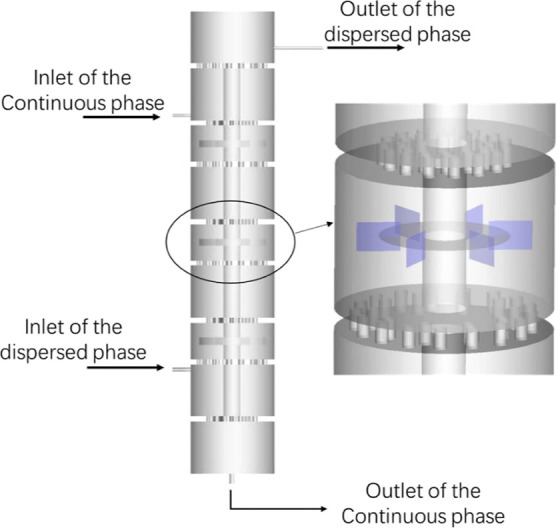
Structure of the three-stage stirred sieve-plate extraction column.
Table 2. Parameters of the Stirred Sieve-Plate Extraction Column.
| geometry | symbol | size (mm) |
|---|---|---|
| diameter of the column | DC | 50 |
| diameter of the agitator | DI | 40 |
| height of the agitator | HI | 7 |
| height of the stirring section | HA | 35 |
| height of the settling section | HS | 50 |
| diameter of the holes | dN | 3 |
| thickness of the sieve plate | TP | 3 |
Table 3. Systems Used in the Simulation.
| no. | continuous phase | dispersed phase | ρc (kg/m3) | ρd (kg/m3) | μc (mPa s) | μd (mPa s) | σ (mN/m) |
|---|---|---|---|---|---|---|---|
| 1 | water | isoamyl alcohol | 995.7 | 846.0 | 0.801 | 3.19 | 4.4 |
| 2 | 30 wt % glycerin aqueous solution | 1-octanol | 1068.5 | 815.3 | 1.816 | 5.069 | 7.7 |
| 3 | water | 1-octanol | 995.7 | 815.3 | 0.801 | 5.069 | 8.4 |
| 4 | water | butyl acetate | 995.7 | 871.6 | 0.801 | 0.607 | 13.9 |
| 5 | 30 wt % glycerin aqueous solution | n-heptane | 1068.5 | 676.2 | 1.816 | 0.376 | 39.2 |
| 6 | water | n-heptane | 995.7 | 676.2 | 0.801 | 0.376 | 49.5 |
3.2. Numerical Schemes
The Ansys ICEM 14.5 was used to generate hexahedral mesh for the computational domain, and the mesh near the impeller, hole, inlet, and outlet was refined. The blade and plate walls were treated as surfaces without thickness. The mesh is presented in Figure 2. The velocity inlet condition was adopted at the inlet, and the velocity outlet condition was adopted at the continuous phase outlet. The outflow boundary was adopted at the dispersed phase outlet to avoid manually specifying the DSD at the outlet.
Figure 2.

Mesh of the column.
The Euler–Euler approach was adopted to model liquid–liquid dispersions in the column, and the RANS equation was adopted to simulate the turbulence. The standard k–ε model is a popular and economic turbulence model for macro flow, which was also adopted in this work. All simulations were carried out in Ansys Fluent 19.2. The steady-state simulation was performed, and the multiple reference frame (MRF) model was specified in the rotating zone. The impeller and shaft walls were set as moving wall conditions, and all the other walls were defined as no-slip wall boundary conditions. The first-order upwind scheme was applied to discretize the flow equations. The phase-coupled SIMPLE algorithm was used for pressure–velocity coupling.
To solve the PBM, the discrete method (DM) was used, which discretized the droplet size into several finite bins. The more the number of bins is, the more possible it is to reflect the DSD in actual conditions; meanwhile, the longer the calculation time will be. Considering the time cost of simulation and based on the previous research on the droplet diameters in the stirred sieve-plate extraction column, the droplet diameters were divided into eight bins. The corresponding diameters of droplets in each bin are shown in Table 4.
Table 4. Discrete Droplet Sizes.
| bin | 0 | 1 | 2 | 3 | 4 | 5 | 6 | 7 |
| d (mm) | 4.064 | 2.560 | 1.613 | 1.016 | 0.640 | 0.403 | 0.254 | 0.160 |
3.3. Grid Independence Test
The grid independence test was carried out for three levels with 1,292,046 cells (grid 1), 2,315,006 cells (grid 2), and 4,009,798 cells (grid 3), using water as the continuous phase and heptane as the dispersed phase, with inlet volume flow rates of 3 and 1 mL/min, respectively. The stirring speed was 480 rpm. Then, the velocity and turbulent kinetic energy of different locations in the second stirring section were compared to select the appropriate grid. The locations used for comparison were line 1 and line 2, as shown in Figure 3, which were 1.5 mm above and 2.5 mm below the blade in the second stirring section, respectively.
Figure 3.

Locations of lines 1 and 2 in the second stirring section.
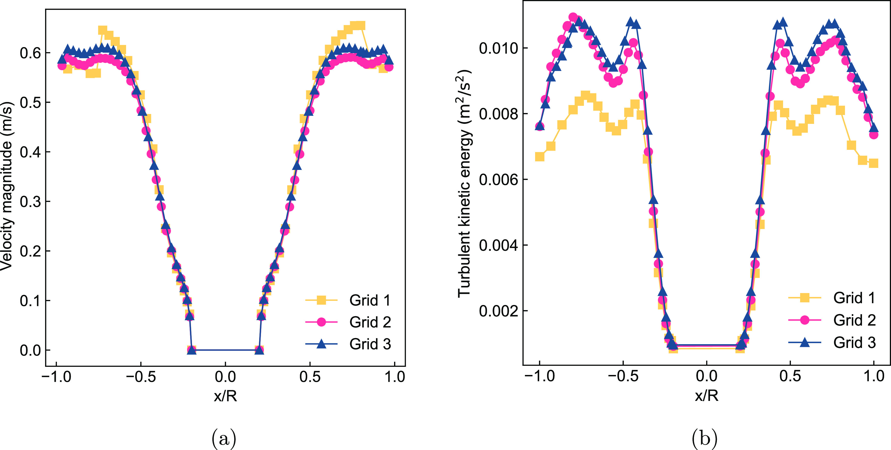
The simulation data at line 1 with different levels of the grid were read and plotted in Figure 4. As can be seen, with the increase in cell number, the velocity and turbulent kinetic energy tend to be stable. The curves of grids 2 and 3 almost coincide, while the curves of grid 1 are slightly deviated due to the small number of cells. It is also found that the fluid velocity increases along the impeller and reaches the maximum value at the outer end of the blade, while the turbulence intensity and the velocity gradient reach the maximum at both ends of the blade, which is consistent with the actual situation.
Figure 4.

Velocity magnitude (a) and turbulent kinetic energy (b) in line 1.
While, as shown in Figure 5, the velocity gradient on line 2 is smaller than that on line 1. Furthermore, the effects of the cell number on the simulation results are similar to that in line 1. The curves of grid 2 and grid 3 generally coincide, whereas the curves of grid 1 show a significant variance.
Figure 5.
Velocity magnitude (a) and turbulent kinetic energy (b) in line 2.
In conclusion, both grid 2 and grid 3 can simulate the stirred sieve-plate extraction column well, while grid 3 requires nearly twice as much computation time as grid 2. Considering the reliability and computation time of the simulation, all subsequent simulations are carried out in grid 2.
4. Results and Discussion
The systems used in this section are listed in Table 3. The CFD-PBM simulations were performed under the same operating conditions as Yuan’s experiment.50 The geometric structure of the extraction column used in the experiment is shown in Figure 1 and Table 2, and the physical properties of the system are shown in Table 3. A pump was used to control the flow rate, after stable operation for 6 h, using the photography method to capture pictures of droplets in the stirring section. By measuring the diameter of approximately 100 droplets and then using the equation below to determine d32.
| 19 |
In addition to using the CT model as the breakage and coalescence kernel, a modified model consisting of the breakage kernel of Zongchang and Caoyong44 and the coalescence kernel of Yu et al.46 is also used.
For different dispersed phases, the modified model needs to be fitted according to the experimental results to obtain the model parameter C3. In this work, C3 was obtained using the experimental data of d32 under the maximum stirring speed. The fitting values are given in Table 5, which also gives the viscosity value of each dispersed phase. It can be seen that C3 generally increases as the dispersed phase viscosity increases.
Table 5. C3 for Different Dispersed Phases.
| dispersed phase | heptane | butyl acetate | isoamyl alcohol | octanol |
|---|---|---|---|---|
| μd (Pa·s) | 0.386 | 0.607 | 3.190 | 5.069 |
| C3 | 10.5 | 8.5 | 20.5 | 40.5 |
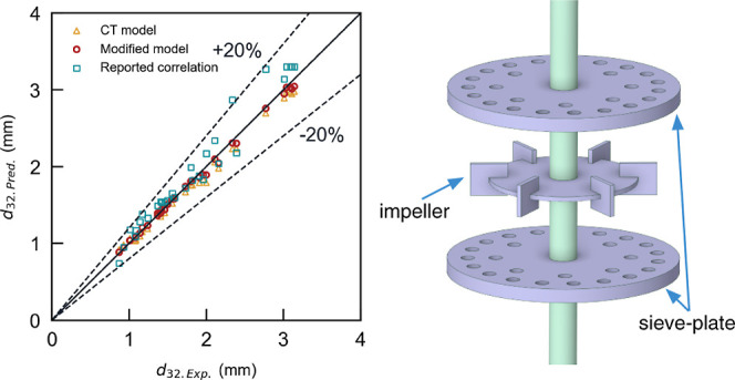
Yuan et al.8 proposed the following empirical correlation to predict the d32 of the dispersed phase in the stirred sieve-plate extraction column, which was also used to compare with the simulation and experimental results.
 |
20 |
4.1. Effect of Stirring Speed
The comparison of d32 acquired from experiment, simulation, and correlation under different stirring speed is presented in Figure 6. It can be seen that the correlation results of eq 20 have a significant deviation from the experimental values, while the CFD-PBM simulation results are closer to the experimental values. This might be attributed to the fact that the coalescence and breakage model used in CFD-PBM is theoretically derived, which, in comparison to empirical formulas, better reflects actual physical phenomena and, consequently, offers higher accuracy. Both simulation and experimental results show that d32 decreases gradually with the increase in stirring speed. As the stirring speed increases, the input power per unit mass of fluid increases, and the turbulence intensity becomes stronger, resulting in a decrease in the diameter of dispersed droplets.
Figure 6.

d32 at different stirring speeds, the experimental data is sourced from Yaun,50 (a) system 1, Qc = 3 mL/min, Qd = 2 mL/min, (b) system 2, Qc = 3 mL/min, Qd = 1 mL/min, (c) system 3, Qc = 3 mL/min, Qd = 1 mL/min, (d) system 4, Qc = 3 mL/min, Qd = 1 mL/min, and (e) system 6, Qc = Qd = 3 mL/min.
To further elucidate the influence of the stirring speed on the hydrodynamic behavior inside the tower, three representative cases from Figure 6e were selected for analysis. Figure 7 shows turbulent kinetic energy contour plots, revealing that in the vicinity of the impeller blades, turbulent kinetic energy is significantly higher due to the rapid rotation of the agitator. Moreover, as the stirring speed increases, the overall turbulent kinetic energy within the stirring section becomes larger.
Figure 7.

Spatial variation of turbulent kinetic energy in the intermediate stirring section (system 6, Qc = Qa = 3 mL/min), (a) N = 460 rpm, (b) N = 540 rpm, and (c) N = 590 rpm.
Turbulent kinetic energy represents the intensity and energy distribution of turbulence, while the turbulent dissipation rate indicates the rate at which turbulence energy dissipates. Figure 8 illustrates the average turbulent dissipation rate in the intermediate stirring section, which exhibits a rapid increase as the stirring speed escalates. This signifies enhanced turbulence instability within the stirring section, facilitating the breakage of liquid droplets.
Figure 8.

Average turbulent dissipation rate in the intermediate stirring section at different stirring speeds (system 6, Qc = Qd = 3 mL/min).
It is worth noting that the simulation accuracy of the modified model considering the effect of the dispersed phase viscosity is better than that of the CT model, which further supports the idea of Zongchang and Caoyong,44 as well as Yu et al.,46 that the viscosity of the dispersed phase plays an important role in the process of droplet breakage and coalescence.
The sole difference between the systems in Figure 6b,c is the continuous phase; all other operating conditions are the same. When utilizing the modified model with the same C3, the simulation results for both systems are quite close to the experimental values, which indicates that C3 is related to dispersed phase properties and independent of continuous phase properties.
4.2. Effect of Flow Rate
This section investigates the behavior of d32 at varying volume flow rates. As depicted in Figure 9, d32 increases with an increase in the dispersed phase volume flow rate. When the stirring speed remains constant, an increase in the dispersed phase flow rate will reduce the turbulent energy per unit volume of the dispersed phase, making the dispersed phase insufficient to break into smaller droplets.
Figure 9.

d32 at different dispersed phase flow rates, the experimental data is sourced from Yaun,50 (a) system 1, Qc = 3 mL/min, N = 200 rpm, (b) system 3, Qc = 3 mL/min, N = 270 rpm, and (c) system 5, Qc = 3 mL/min, N = 440 rpm.
Three representative cases were selected from Figure 9b for analyzing their hydrodynamic performance. Figures 10 and 11, respectively, depict the spatial variation of the turbulent kinetic energy and the average turbulent dissipation rate for the intermediate stirring section. It can be observed from Figure 10 that, unlike the significant influence of stirring speed on turbulence, an increase in the dispersed phase flow rate does not result in a substantial increase in turbulent kinetic energy. As shown in Figure 11, with the increase in the dispersed phase flow rate, the turbulent dissipation rate gradually decreases. This may be attributed to the fact that although a higher dispersed phase flow rate promotes the accumulation of energy in large-scale turbulent vortices, resulting in higher turbulent kinetic energy, a turbulent dissipation rate is associated with small-scale vortex structures. Due to a constant stirring speed, the additional energy input is insufficient, which limits the transfer of turbulent energy from large-scale vortices to small-scale vortices. Nevertheless, the magnitude of the turbulent dissipation rate variation is much smaller compared with Figure 8. As a result, when the dispersed phase flow rate is tripled in Figure 9b, the d32 value increases by only around 10%.
Figure 10.

Spatial variation of turbulent kinetic energy in the intermediate stirring section (system 3, Qc = 3 mL/min, N = 270 rpm), (a) Qd = 1 mL/min, (b) Qd = 3 mL/min, and (c) Qd = 5 mL/min.
Figure 11.

Average turbulent dissipation rate in the intermediate stirring section at different dispersed phase flow rates (system 3, Qc = 3 mL/min, N = 270 rpm).
Furthermore, it can be observed that, under the same flow rate, the stirring speed in Figure 9c is 440 rpm, which is higher than that in Figure 9a,b. However, the value of d32 is the highest in Figure 9c. This discrepancy arises from the different systems used; system 5 has a surface tension of 39.2 mN/m, significantly greater than systems 1 and system 3. Higher surface tension makes droplet breakup more difficult, which is why system 5 still maintains a larger d32 even at the higher stirring speed of 440 rpm. In contrast, system 1 has a surface tension of only 4.4 mN/m, making droplets easier to break up.
To explore the influence of continuous phase flow rate on dispersed phase droplet diameter, the dispersed phase volume flow rate is kept at 1 mL/min for system 5, the stirring speed at 350 rpm, and the d32 under different continuous phase volume flow rates, as shown in Figure 12. It can be observed that with an increase in the continuous phase flow rate, the variation in d32 is not significant, which is consistent with the results obtained by other researchers.7,8,30,51,52
Figure 12.

d32 at different continuous phase flow rates, the experimental data is sourced from Yaun,50 system 5, Qd = 1 mL/min, N = 350 rpm.
Based on Figures 9 and 12, it is clear that the modified model still has the highest simulation accuracy. This further highlights the importance of taking into account the viscosity of the dispersed phases.
5. Conclusions
In this work, a CFD-PBM coupled simulation method was established to simulate d32 in a three-stage stirred sieve-plate extraction column.
The variance between the simulated d32 and the experimental data when the CT model is used as kernel functions is less than 10%, as opposed to a 20% deviation when using the correlation equation. On this basis, for different dispersed phases, a modified model considering the viscosity of the dispersed phase was used, in which the model parameter for the dispersed phase is obtained by fitting it with experimental data. The results show that for different systems, the simulation and experimental results agree well, with a variance of less than 5%, demonstrating the modified model’s broad applicability. For the systems with the same dispersed phase and different continuous phases, the same model parameter is applicable, indicating that the model parameter is only related to the properties of the dispersed phase and has nothing to do with the continuous phase. In addition, the simulated results show that d32 decreases with the increase in stirring speed and increases with the increase of the dispersed phase flow rate, and the increase in continuous phase flow rate does not have a significant impact on d32. The results presented in this study will provide useful references for users and designers of stirred sieve-plate extraction columns or extraction columns with similar structures.
Acknowledgments
This work was supported by the development and industrialization of high-performance, fine-denier polyphenylene sulfide (PPS) fiber (2023C01094), Zhejiang Province “Jianbing” “Lingyan” research and development plan.
The authors declare no competing financial interest.
References
- Scheibel E. G. Fractional liquid extraction. Chem. Eng. Prog. 1948, 44, 681–690. [Google Scholar]
- Scheibel E. G. Performance of an internally baffled multistage extraction column. AIChE J. 1956, 2, 74–78. 10.1002/aic.690020116. [DOI] [Google Scholar]
- Pang K.; Johnson A. Mathematical modeling of a modified scheibel liquid-liquid extraction column in the frequency domain. Can. J. Chem. Eng. 1971, 49, 837–843. 10.1002/cjce.5450490622. [DOI] [Google Scholar]
- Bonnet J.; Jeffreys G. Hydrodynamics and mass transfer characteristics of a Scheibel extractor. Part I: Drop size distribution, holdup, and flooding. AIChE J. 1985, 31, 788–794. 10.1002/aic.690310513. [DOI] [Google Scholar]
- Chen Z. S.; Yuan S. F.; Yin H.; Chen Z. R. Study on a modified Scheibel extraction column. Zhejiang Chem. Ind. 2010, 41, 23–26. [Google Scholar]
- Yin H.; Chen Z. S.; Yuan S. F.; Chen Z. R. Study on an ideal start-up model for a modified Scheibel column. Appl. Math. Models 2011, 35, 5835–5841. 10.1016/j.apm.2011.05.028. [DOI] [Google Scholar]
- Yuan S.; Shi Y.; Yin H.; Chen Z. R.; Zhou J. Z. Correlation of the drop size in a modified scheibel extraction column. Chem. Eng. Technol. 2012, 35, 1810–1816. 10.1002/ceat.201100470. [DOI] [Google Scholar]
- Yuan S. f.; Jin S. f.; Chen Z. r.; Yuan Y. n.; Yin H. An improved correlation of the mean drop size in a modified scheibel extraction column. Chem. Eng. Technol. 2014, 37, 2165–2174. 10.1002/ceat.201300873. [DOI] [Google Scholar]
- Shi Y.; Yuan S. F.; Yin H.; Chen Z. R. An RTD model of dispersed phase in a modified Scheibel extraction column. J. Zhejiang Univ., Sci., A 2013, 40, 191–195. [Google Scholar]
- Yuan Y. N.; Yuan S. F.; Chen Z. R.; Shi Y.; Hong Y. A nonequilibrium stage model of the modified Scheibel extraction column. J. Zhejiang Univ., Sci., A 2014, 41, 181–184. [Google Scholar]
- Shen-feng Y.; Zhi-peng L.; Hong Y.; Zhi-rong C. Study on flooding characteristics in an agitated sieve plate extraction column. Chem. J. Chin. Univ. 2021, 35, 601–607. [Google Scholar]
- Shen-feng Y.; Zhi-peng L.; Hong Y.; Zhi-rong C. Study on droplet size in an agitated sieve-plate extraction column. Chem. J. Chin. Univ. 2021, 35, 986–993. [Google Scholar]
- Bujalski J.; Yang W.; Nikolov J.; Solnordal C.; Schwarz M. Measurement and CFD simulation of single-phase flow in solvent extraction pulsed column. Chem. Eng. Sci. 2006, 61, 2930–2938. 10.1016/j.ces.2005.10.057. [DOI] [Google Scholar]
- Drumm C.; Bart H. J. Hydrodynamics in a RDC extractor: Single and two-phase PIV measurements and CFD simulations. Chem. Eng. Technol. 2006, 29, 1297–1302. 10.1002/ceat.200600212. [DOI] [Google Scholar]
- Drumm C.; Hlawitschka M. W.; Bart H.-J. CFD simulations and particle image velocimetry measurements in an industrial scale rotating disc contactor. AIChE J. 2011, 57, 10–26. 10.1002/aic.12249. [DOI] [Google Scholar]
- Sen N.; Singh K. K.; Patwardhan A. W.; Mukhopadhyay S.; Shenoy K. T. CFD simulations of pulsed sieve plate column: axial dispersion in single-phase flow. Sep. Sci. Technol. 2015, 50, 2485–2495. 10.1080/01496395.2015.1064136. [DOI] [Google Scholar]
- Yi H.; Wang Y.; Smith K. H.; Fei W.; Stevens G. W. CFD simulation of liquid–liquid two-phase hydrodynamics and axial dispersion analysis for a non-pulsed disc and doughnut solvent extraction column. Solvent Extr. Ion Exch. 2016, 34, 535–548. 10.1080/07366299.2016.1226025. [DOI] [Google Scholar]
- Sen N.; Singh K.; Patwardhan A.; Mukhopadhyay S.; Shenoy K. CFD simulation of two-phase flow in pulsed sieve-plate column–Identification of a suitable drag model to predict dispersed phase hold up. Sep. Sci. Technol. 2016, 51, 2790–2803. 10.1080/01496395.2016.1218895. [DOI] [Google Scholar]
- Sen N.; Singh K.; Patwardhan A.; Mukhopadhyay S.; Shenoy K. CFD simulations to predict dispersed phase holdup in a pulsed sieve plate column. Sep. Sci. Technol. 2018, 53, 2587–2600. 10.1080/01496395.2018.1459702. [DOI] [Google Scholar]
- Farakte R. A.; Hendre N. V.; Patwardhan A. W. CFD simulations of two phase flow in asymmetric rotary agitated columns. Ind. Eng. Chem. Res. 2018, 57, 17192–17208. 10.1021/acs.iecr.8b02720. [DOI] [Google Scholar]
- Hinge S. P.; Patwardhan A. W. Hydrodynamics aspects of asymmetric rotating impeller columns at different scales. Chem. Eng. Res. Des. 2022, 177, 625–639. 10.1016/j.cherd.2021.11.022. [DOI] [Google Scholar]
- Sarkar S.; Singh K.; Shenoy K. Axial dispersion and pressure drop for single-phase flow in annular pulsed disc and doughnut columns: A CFD study. Prog. Nucl. Energy 2018, 106, 335–344. 10.1016/j.pnucene.2018.03.003. [DOI] [Google Scholar]
- Sarkar S.; Singh K. K.; Shenoy K. T. CFD modeling of pulsed disc and doughnut column: prediction of axial dispersion in pulsatile liquid–liquid two-phase flow. Ind. Eng. Chem. Res. 2019, 58, 15307–15320. 10.1021/acs.iecr.9b01465. [DOI] [Google Scholar]
- Yuan S.; Jin L.; Chen Z.; Yin H. Structural optimization and flow field analysis of agitated extraction column based on CFD. Chin. J. Process Eng. 2023, 23, 681–690. [Google Scholar]
- Chen H.; Sun Z.; Song X.; Yu J. Key parameter prediction and validation for a pilot-scale rotating-disk contactor by CFD–PBM simulation. Ind. Eng. Chem. Res. 2014, 53, 20013–20023. 10.1021/ie503115w. [DOI] [Google Scholar]
- Chen H.; Sun Z.; Song X.; Yu J. Operating Regimes and Hydrodynamics of a Rotating-Disc Contactor. Chem. Eng. Technol. 2017, 40, 498–505. 10.1002/ceat.201500295. [DOI] [Google Scholar]
- Sen N.; Singh K.; Patwardhan A.; Mukhopadhyay S.; Shenoy K. CFD-PBM simulations of a pulsed sieve plate column. Prog. Nucl. Energy 2019, 111, 125–137. 10.1016/j.pnucene.2018.10.012. [DOI] [Google Scholar]
- Sarkar S.; Singh K. K.; Mahajani S.; Trivikram Shenoy K. CFD-PB modelling of liquid–liquid two-phase flow in pulsed disc and doughnut column. Solvent Extr. Ion Exch. 2020, 38, 536–554. 10.1080/07366299.2020.1767360. [DOI] [Google Scholar]
- Yu X.; Zhou H.; Jing S.; Lan W.; Li S. Augmented CFD–PBM simulation of liquid–liquid two-phase flows in liquid extraction columns with wettable internal plates. Ind. Eng. Chem. Res. 2020, 59, 8436–8446. 10.1021/acs.iecr.0c01476. [DOI] [Google Scholar]
- Tan B.; Lan M.; Li L.; Wang Y.; Qi T. Drop size correlation and population balance model for an agitated-pulsed solvent extraction column. AIChE J. 2020, 66, e16279 10.1002/aic.16279. [DOI] [Google Scholar]
- Tan B.; Wang B.; Chang C.; Wang Y.; Zheng S.; Qi T. Hydrodynamic Behavior Analysis of Agitated-Pulsed Column by CFD-PBM. Solvent Extr. Ion Exch. 2022, 40, 518–539. 10.1080/07366299.2021.2004660. [DOI] [Google Scholar]
- Luo H.; Svendsen H. F. Theoretical model for drop and bubble breakup in turbulent dispersions. AIChE J. 1996, 42, 1225–1233. 10.1002/aic.690420505. [DOI] [Google Scholar]
- Laakkonen M.; Alopaeus V.; Aittamaa J. Validation of bubble breakage, coalescence and mass transfer models for gas-liquid dispersion in agitated vessel. Chem. Eng. Sci. 2006, 61, 218–228. 10.1016/j.ces.2004.11.066. [DOI] [Google Scholar]
- Coulaloglou C.; Tavlarides L. L. Description of interaction processes in agitated liquid-liquid dispersions. Chem. Eng. Sci. 1977, 32, 1289–1297. 10.1016/0009-2509(77)85023-9. [DOI] [Google Scholar]
- Sovova H. Breakage and coalescence of drops in a batch stirred vessel—II comparison of model and experiments. Chem. Eng. Sci. 1981, 36, 1567–1573. 10.1016/0009-2509(81)85117-2. [DOI] [Google Scholar]
- Prince M. J.; Blanch H. W. Bubble coalescence and break-up in air-sparged bubble columns. AIChE J. 1990, 36, 1485–1499. 10.1002/aic.690361004. [DOI] [Google Scholar]
- Liao Y.; Lucas D. A literature review of theoretical models for drop and bubble breakup in turbulent dispersions. Chem. Eng. Sci. 2009, 64, 3389–3406. 10.1016/j.ces.2009.04.026. [DOI] [Google Scholar]
- Liao Y.; Lucas D. A literature review on mechanisms and models for the coalescence process of fluid particles. Chem. Eng. Sci. 2010, 65, 2851–2864. 10.1016/j.ces.2010.02.020. [DOI] [Google Scholar]
- Maaß S.; Kraume M. Determination of breakage rates using single drop experiments. Chem. Eng. Sci. 2012, 70, 146–164. 10.1016/j.ces.2011.08.027. [DOI] [Google Scholar]
- Gao Z.; Li D.; Buffo A.; Podgórska W.; Marchisio D. L. Simulation of droplet breakage in turbulent liquid–liquid dispersions with CFD-PBM: Comparison of breakage kernels. Chem. Eng. Sci. 2016, 142, 277–288. 10.1016/j.ces.2015.11.040. [DOI] [Google Scholar]
- Shih T.-H.; Liou W. W.; Shabbir A.; Yang Z.; Zhu J. A new k-ϵ eddy viscosity model for high reynolds number turbulent flows. Comput. Fluids 1995, 24, 227–238. 10.1016/0045-7930(94)00032-t. [DOI] [Google Scholar]
- Wang F.; Mao Z. S. Numerical and experimental investigation of liquid- liquid two-phase flow in stirred tanks. Ind. Eng. Chem. Res. 2005, 44, 5776–5787. 10.1021/ie049001g. [DOI] [Google Scholar]
- Schiller L.; Naumann A. A drag coefficient correlation. Z. Ver. Dtsch. Ing. 1935, 77, 318–320. [Google Scholar]
- Zongchang Z.; Caoyong Y. Modified viscosity model of droplet breakage frequency for turbulent liquid-liquid dispersions. CIESC J. 2006, 57, 2834. [Google Scholar]
- Hill P. J.; Ng K. M. New discretization procedure for the breakage equation. AIChE J. 1995, 41, 1204–1216. 10.1002/aic.690410516. [DOI] [Google Scholar]
- Yu S.-B.; Zhao Z.-C.; Yin C.-Y. The simulation of the drop sizes in turbulent liquid-liquid dispersions. Chem. J. Chin. Univ. 2008, 22, 574–579. [Google Scholar]
- Tobin T.; Ramkrishna D. Modeling the effect of drop charge on coalescence in turbulent liquid—liquid dispersions. Can. J. Chem. Eng. 1999, 77, 1090–1104. 10.1002/cjce.5450770603. [DOI] [Google Scholar]
- Ross S. L.; Curl R. L.. Measurement and models of the dispersed phase mixing process. Paper no. 29b. 4th International Chemical Engineering Conference: Vancouver, 1973.
- Coulaloglou C. A.Dispersed Phase Interactions in an Agitated Flow Vessel. Ph.D. thesis, Illinois Institute of Technology, Chicago, 1975. [Google Scholar]
- Yuan Y. N.Study on two-phase flow behavior of improved Scheibel extraction column. M.Sc. thesis, ZheJiang University, Hangzhou, 2013. [Google Scholar]
- Hemmati A.; Torab-Mostaedi M.; Shirvani M.; Ghaemi A. A study of drop size distribution and mean drop size in a perforated rotating disc contactor (PRDC). Chem. Eng. Res. Des. 2015, 96, 54–62. 10.1016/j.cherd.2015.02.005. [DOI] [Google Scholar]
- Weber B.; Schneider M.; Görtz J.; Jupke A. Compartment model for liquid-liquid extraction columns. Solvent Extr. Ion Exch. 2020, 38, 66–87. 10.1080/07366299.2019.1691137. [DOI] [Google Scholar]