

Abstract
This paper examines the long-run effects of the 1980–1982 recession on education and income. Using confidential Census data, I estimate difference-in-differences regressions that exploit variation across counties in recession severity and across cohorts in age at the time of the recession. For individuals age 0–10 in 1979, a 10 percent decrease in earnings per capita in their county of birth reduces four-year college degree attainment by 15 percent and earnings in adulthood by 5 percent. Simple calculations suggest that, in aggregate, the 1980–1982 recession led to 1.3–2.8 million fewer college graduates and $66–$139 billion less earned income per year.
JEL Classification Codes: E32, I20, I30, J13, J24
Keywords: human capital, education, income, recessions
1. Introduction
Recessions receive tremendous attention from economists, policymakers, and the public. Most of this attention focuses on the short-run effects of recessions on workers’ labor market outcomes and firms’ investment and employment decisions. In addition to these short-run effects, recessions could have consequential long-run effects, especially if they affect human capital attainment. Influential theoretical and empirical work emphasizes the role of opportunity cost: by reducing labor market opportunities, recessions might increase educational attainment (Mincer, 1958; Becker, 1962; Black, McKinnish and Sanders, 2005; Atkin, 2016; Charles, Hurst and Notowidigdo, 2018; Cascio and Narayan, 2019).
The opportunity cost channel is most relevant for individuals making high school and college enrollment decisions during the recession. However, recessions could affect younger individuals, for whom mechanisms besides opportunity cost, such as a decrease in human capital investments during childhood, might dominate. Consequently, the size and even sign of long-run effects are an empirical question. This paper estimates the long-run effects of recessions on education and income for individuals who were children, adolescents, and young adults when the recession began.
I focus on the 1980–1982 double-dip recession in the United States, which followed large increases in interest rates and the price of oil. The recession was concentrated in certain industries, like durable goods manufacturing and wood products, and counties with pre-existing specialization in these industries experienced a more severe recession. The 1980–1982 recession is a valuable setting because its timing permits the study of counties’ pre-recession economic conditions and individuals’ long-run outcomes. I show that the recession led to a persistent relative decrease in earnings per capita and median family income in negatively affected counties. This persistent decrease in local economic activity is central in considering the long-run effects on individuals.
I estimate the long-run effects of the recession using newly available confidential data. I link the 2000 Census and 2001–2013 American Community Surveys to the Social Security Administration NUMIDENT file, which allows me to observe outcomes in adulthood and county of birth for 23 million individuals born from 1950–1979. With these data, I estimate generalized difference-in-differences regressions that compare education and income in adulthood of individuals born in counties with a more versus less severe recession (first difference) and individuals who were younger versus older when the recession began (second difference). I isolate the effect of local labor demand shifts that emerged during the recession by instrumenting for the 1979–1982 change in log real earnings per capita with the log employment change predicted by the interaction of a county’s pre-existing industrial structure and aggregate employment changes. This empirical strategy identifies the overall effect of the recession on long-run outcomes, inclusive of any mitigating actions by parents and communities.1
I find that the 1980–1982 recession led to sizable long-run reductions in education and income. For individuals age 0–10 in 1979, a 10 percent decrease in real earnings per capita in their county of birth, which is around one standard deviation, leads to a 4.4 percentage point (14.6 percent) decrease in four-year college degree attainment. The negative effects on college graduation are most severe and essentially constant for individuals age 0–13 in 1979. This age profile suggests that the underlying mechanisms are a decline in childhood human capital or a long-term decline in parental resources to pay for college. Because I estimate small and statistically insignificant effects on college graduation for individuals age 14–19 in 1979, short-term credit constraints in paying for college appear less important. I estimate smaller negative impacts on college attendance and find no evidence of an effect on high school graduation. For individuals age 0–10 in 1979, a 10 percent decrease in real earnings per capita leads to a $2,100 (5.2 percent) decrease in earned income, a $1,900 (4.5 percent) decrease in total income, and a 1.6 percentage point (13.0 percent) increase in the probability of living in poverty from 2000–2013. Simple calculations suggest that much of the long-run effects on income stem from the effects on education.
An important question is whether government policies mitigated these long-run effects. To study this, I characterize several relevant dimensions of state transfer systems as of 1970. I examine transfer generosity using total transfers and state appropriations to higher education, conditional on standard economic and demographic variables. In addition, I measure transfer progressivity as the degree to which states transferred higher amounts to poorer counties, conditional on standard variables. I find little evidence that states with more generous or more progressive transfer systems mitigated the long-run effects.
Several pieces of evidence support the validity of my empirical strategy. First, I show that earnings per capita evolved similarly before 1980 in counties with a more versus less severe recession. Second, I find no evidence of a relationship between the severity of the recession and the evolution of infant mortality—a marker of early life health and human capital—from 1950–1979. Most importantly, I conduct falsification tests by estimating the effect of the recession on education for individuals age 23–28 in 1979, using 29 year olds as a comparison group. I find no evidence of an effect for 23–28 year olds, who largely completed their schooling before the recession. These findings strongly support my research design.
The magnitude of my estimates and the large number of affected individuals suggest that the 1980–1982 recession depresses aggregate economic output today. To gauge the aggregate effects, I scale my estimates by the 70 million individuals born in the U.S. from 1960–1979. Depending on the assumed evolution of earnings per capita in the absence of the recession, back of the envelope calculations suggest that the 1980–1982 recession led to 1.3–2.8 million fewer four-year college graduates, $66–$139 billion less earned income per year (as of 2000–2013), and 0.4–0.9 million more adults living in poverty each year. These numbers represent 2–4 percent of the stock of college-educated adults, 0.4–0.8 percent of GDP, and 1–2 percent of the number of individuals in poverty in 2015. While these calculations could understate or overstate the true aggregate effects, as I discuss in detail, the long-run effects that I document are important channels through which recessions affect welfare and economic growth.
This paper shows that the 1980–1982 recession persistently decreased earnings per capita in negatively affected counties, and children and adolescents born in these counties have less education and income as adults. In addition, I show that every U.S. recession since 1973 has persistently decreased earnings per capita in negatively affected counties. This novel stylized fact indicates that the 1980–1982 recession is not unique in its persistent effects on county-level earnings per capita, which suggests that it might not be unique in its long-run effects on human capital attainment. Similar long-run effects could arise from other shocks leading to persistent declines in local economic activity, such as Chinese import competition (Autor, Dorn and Hanson, 2013) and NAFTA (McLaren and Hakobyan, 2016).
This paper contributes to four distinct literatures. First is the literature on the effect of labor market opportunities on contemporaneous schooling enrollment, with a focus on the role of opportunity cost (Black, McKinnish and Sanders, 2005; Atkin, 2016; Charles, Hurst and Notowidigdo, 2018; Cascio and Narayan, 2019). I complement this literature by estimating effects on a wider age range, including children and adolescents, which is possible because of newly available data.2
Second is the literature on the role of early life conditions in shaping human capital and productivity (for recent reviews, see Almond and Currie, 2011; Heckman and Mosso, 2014; Almond, Currie and Duque, 2018). This literature provides very little direct evidence on the long-run effects of recessions on education and income.3 Furthermore, Chetty and Hendren (2018b) find little relationship between local economic conditions and the effect of a place on children’s long-run outcomes. As a result, considerable uncertainty exists about the magnitude and sign of recessions’ long-run effects. Evidence on the size of these effects is necessary for weighing the potential benefits of mitigating policies, and for assessing whether these long-run effects should be incorporated into theoretical and empirical models of recessions and the economy. My primary contribution is estimating the long-run effects of a recession on education and income. I find that the long-run effects on children’s and adolescents’ income are more severe than the effects on individuals entering or already in the labor market at the time of the recession.4
This paper also contributes to work on the welfare costs of recessions. Most of this literature focuses on the costs of intertemporal substitution in consumption (see the review in Lucas, 2003). In contrast, I study costs that stem from long-run declines in children’s and adolescents’ human capital attainment. My results imply that recessions are costlier than previously thought and point to new possible targets for social insurance and economic stabilization policies.5 Finally, this paper contributes to the literature studying how recessions affect subsequent economic activity. An influential strand of this literature examines recessions’ cleansing effects, which increase productivity as less productive firms exit and resources are reallocated to remaining firms (e.g., Schumpeter, 1939, 1942; Caballero and Hammour, 1994; Davis, Haltiwanger and Schuh, 1996; Foster, Grim and Haltiwanger, 2016). My results demonstrate that recessions also affect productivity in a markedly different way, by reducing children’s and adolescents’ human capital.
2. Background: The 1980–1982 Recession
The 1980–1982 double-dip recession had sizable short-run effects on the U.S. economy.6 The recession followed large increases in interest rates and the price of oil, as Paul Volcker and the Federal Reserve fought inflation and the Iranian Revolution curbed oil production and created panic in energy markets. The unemployment rate was stable from 1978–1980, then increased from 6.3 percent in January 1980 to 10.8 percent in November 1982. As seen in Table 1, employment declines were concentrated in certain industries. The manufacturing sector lost 1.7 million jobs from 1979–1982, and the construction sector lost nearly 600,000 jobs. Within manufacturing, two-thirds of the job loss occurred in six industries, including transportation equipment, primary metal (which includes steel mills) and fabricated metal, lumber and wood products, and textile products. Not all industries experienced employment declines, with notable growth in the mining sector (which includes oil and gas extraction) and the service sector.7
Table 1:
Aggregate Employment Changes from 1979–1982, by Industry
| Share of total 1979 employment | Log employment change | Employment change | |
|---|---|---|---|
| (1) | (2) | (3) | |
| Panel A. Overall and one-digit industries | |||
| All industries | 1.000 | 0.006 | 467,093 |
| Manufacturing | 0.284 | −0.084 | −1,684,627 |
| Construction | 0.061 | −0.139 | −575,107 |
| Agriculture, forestry, and fisheries | 0.004 | 0.131 | 40,200 |
| Transportation and public utilities | 0.062 | 0.013 | 59,944 |
| Wholesale trade | 0.071 | 0.016 | 83,149 |
| Mining | 0.013 | 0.229 | 239,923 |
| Retail trade | 0.203 | 0.017 | 257,134 |
| Finance, insurance, and real estate | 0.070 | 0.060 | 316,449 |
| Services | 0.224 | 0.120 | 2,090,186 |
| Panel B. Two-digit industries with largest employment decrease | |||
| Transportation equipment (manufacturing) | 0.024 | −0.180 | −279,883 |
| General contractors (construction) | 0.018 | −0.223 | −250,039 |
| Special trade contractors (construction) | 0.034 | −0.108 | −242,341 |
| Auto dealers (retail trade) | 0.027 | −0.131 | −232,032 |
| Primary metal (manufacturing) | 0.016 | −0.222 | −229,097 |
| Fabricated metal products (manufacturing) | 0.024 | −0.117 | −188,465 |
| Lumber and wood products (manufacturing) | 0.011 | −0.276 | −181,995 |
| Trucking and warehousing (transportation) | 0.019 | −0.116 | −146,868 |
| Apparel and other textile products (manufacturing) | 0.019 | −0.106 | −129,917 |
| Textile mill products (manufacturing) | 0.012 | −0.161 | −126,208 |
| Panel C. Two-digit industries with largest employment increase | |||
| Legal services (services) | 0.007 | 0.200 | 109,155 |
| Educational services (services) | 0.016 | 0.095 | 114,630 |
| Hotels (services) | 0.014 | 0.110 | 116,017 |
| Depository institutions (finance) | 0.020 | 0.093 | 140,356 |
| Food stores (retail trade) | 0.031 | 0.087 | 196,198 |
| Miscellaneous services (services) | 0.012 | 0.251 | 242,976 |
| Oil and gas extraction (mining) | 0.005 | 0.506 | 249,725 |
| Eating and drinking places (retail trade) | 0.060 | 0.065 | 283,524 |
| Business services (services) | 0.041 | 0.126 | 382,400 |
| Health services (services) | 0.071 | 0.157 | 845,784 |
Notes: I construct this table by aggregating county-level data for the continental United States. Because employment is often suppressed at the county-level, I impute employment using the number of establishments and nationwide information on average employment by establishment size, as described in Appendix C. Source: Census County Business Patterns
To measure the effect of the recession on local economic activity, I use Bureau of Economic Analysis (BEA) data on earnings per capita. Total earnings of a county’s residents, available starting in 1969, primarily comes from administrative unemployment insurance and tax data. The earnings concept is comprehensive, including income from the labor market and asset ownership, and the denominator of earnings per capita comes from Census annual population estimates. Throughout, I use the CPI-U to express all monetary variables in 2014 dollars. For each county, I measure the severity of the recession as the 1979–1982 decrease in log real earnings per capita. This variable captures several ways a recession might affect a county’s residents, such as extensive margin employment changes, replacement of full-time with part-time jobs, replacement of high-wage with low-wage jobs, and decreasing wages or hours within a job.
Figure 1 shows that the severity of the recession varied considerably across counties. Categories on the map correspond to deciles, with darker shades of red indicating a more severe recession. Twenty percent of counties experienced a decline in earnings per capita of 13.4 percent or more, while twenty percent saw earnings growth.8 The map displays regional patterns in recession severity that mirror patterns in industrial specialization. Oil-exporting states, like Kansas, Oklahoma, and Texas, benefited from high oil prices, and states specializing in durable goods manufacturing, like Indiana, Michigan, and Ohio, saw particularly large declines. New England, with more high tech and defense manufacturing, fared relatively well, while the Pacific Northwest, which specialized in logging, fared poorly. Parts of the agricultural upper Midwest also fared poorly, in conjunction with the “farm crisis” (Barnett, 2000). Although the regional patterns are visually striking, 96 percent of the variation in the severity of the recession is within-region and 81 percent is within-state.
Figure 1: Change in Log Real Earnings per Capita, 1979–1982.
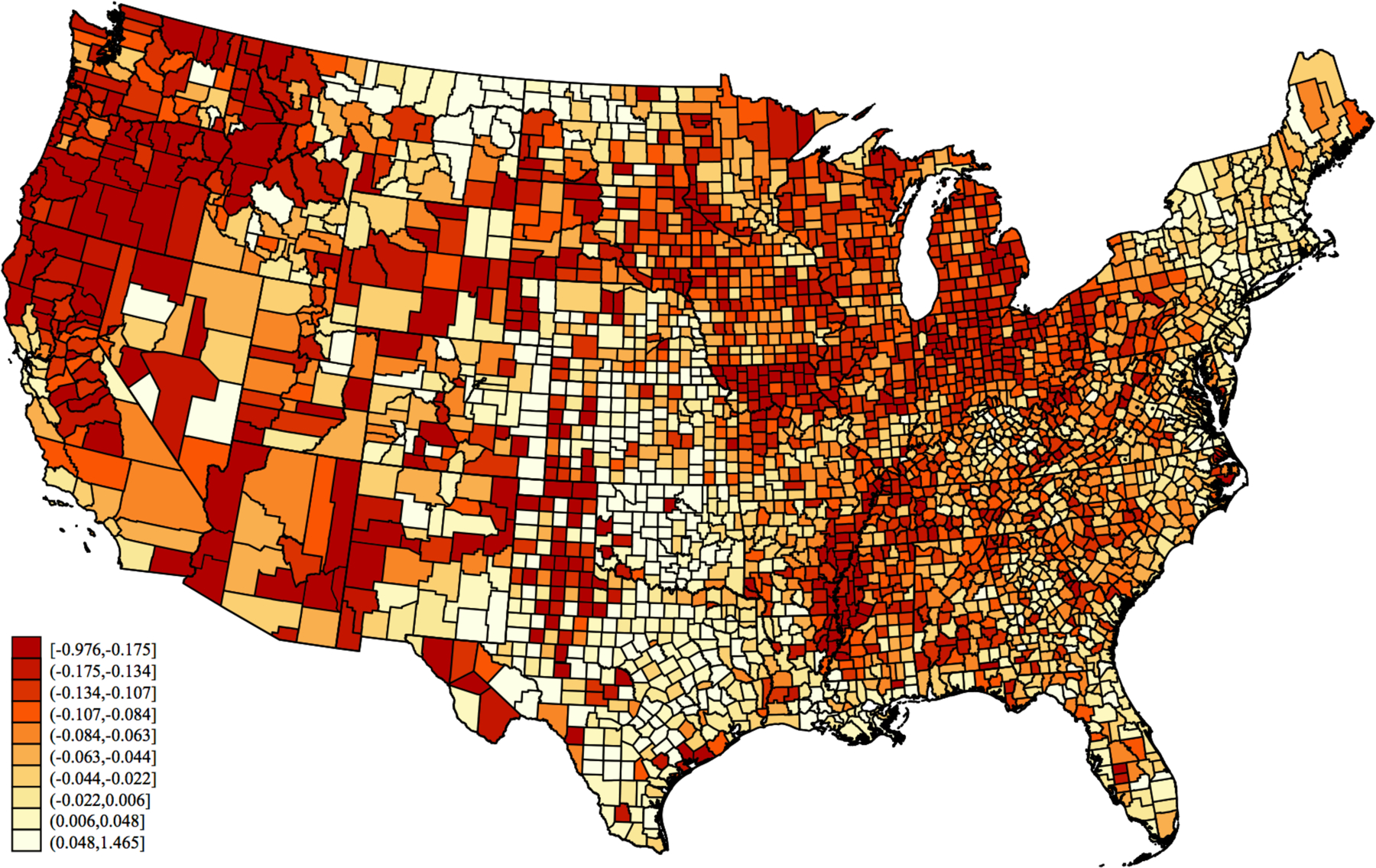
Notes: Figure displays the county-level change in log real earnings per capita from 1979–1982, which I use to measure the severity of the 1980–1982 recession. Categories correspond to unweighted deciles, with darker shades of red representing a larger earnings decrease.
Source: BEA Regional Economic Accounts
Earnings per capita declined suddenly in counties where the recession was more severe, and the relative earnings decline between more versus less severe recession counties has persisted. To show this simply, Figure 2 plots population-weighted mean earnings per capita for counties with a recession more and less severe than the nationwide (1979 population-weighted) median. I shift the less severe recession line down by $2,179, so that the two lines are equal in 1979, to focus on the evolution of earnings per capita over time. Mean earnings per capita evolves identically in more versus less severe recession counties from 1969–1979, then diverges with the onset of the recession. From 1979–1982, mean earnings per capita falls by $2,288 (8.9 percent) in more severe recession counties, while increasing by $76 (0.3 percent) in less severe recession counties. After 1982, mean earnings per capita evolves similarly in both sets of counties, including during later recessions, leaving severe recession counties with a persistent relative decline.9 In the conclusion, I establish the novel stylized fact that every recession in the U.S. since 1973 generates a pattern similar to Figure 2. The employment-population ratio displays a similar pattern (Appendix Figure A.1).
Figure 2: Normalized Mean Real Earnings per Capita, by County-Level Severity of the 1980–1982 Recession.

Notes: Figure displays population-weighted mean real earnings per capita, among counties with a below and above median 1979–1982 decrease in log real earnings per capita. I calculate the median using 1979 population weights. I adjust the less severe recession line to equal the more severe recession line in 1979, which amounts to a downward shift of $2,179. Sample contains 3,076 counties in the continental U.S.
Source: BEA Regional Economic Accounts
The persistence of the relative decline in Figure 2 might seem surprising, given the conventional wisdom, based largely on Blanchard and Katz (1992), that local wages and employment rates converge after negative labor demand shocks. However, several studies find lasting wage and employment rate reductions (Bartik, 1991, 1993; Bound and Holzer, 2000; Greenstone and Looney, 2010; Autor, Dorn and Hanson, 2013; Dix-Carneiro and Kovak, 2017; Yagan, 2019), and economic forces can rationalize this finding. For example, a recession could catalyze a lasting reduction in economic activity by inducing employers to pay fixed adjustment costs and shut down or move to other areas (Foote, 1998).10 Greater out-migration rates or lower in-migration rates of high income workers following a decrease in local labor demand also could contribute to a persistent decrease in earnings per capita (Topel, 1986; Bound and Holzer, 2000; Notowidigdo, 2013). Quantifying the sources of the persistent relative decline is beyond the scope of this paper. Instead, I focus on the long-run effects of the recession on children and adolescents.
3. Possible Long-Run Effects of a Recession on Education and Income
This section draws on previous theoretical and empirical work to describe the possible long-run effects of a recession on education and income. Economic theory does not provide a sharp prediction about the magnitude or even sign of long-run effects, but it does highlight potential channels.
A recession could affect educational attainment and lifetime income by increasing or decreasing human capital obtained during childhood. The stock of childhood human capital depends on material and time investments from parents, community investments from schools, neighborhoods, and peers, and an initial human capital endowment (Almond and Currie, 2011; Heckman and Mosso, 2014). A recession-induced decrease in the local wage could produce income and substitution effects. The income effect predicts a decrease in parents’ material investments.11 The substitution effect, due to a decrease in the cost of spending time with children, predicts an increase in parents’ time investments.12 Community investments could fall due to a reduction in government expenditures or the quality of schools, neighborhoods, or peers.13 I focus on individuals born before 1980, for whom the recession does not affect initial human capital endowments.
A recession could influence high school or college degree attainment independently of any effects on childhood human capital. In choosing their desired level of schooling, individuals trade off higher lifetime earnings against the opportunity cost of forgone earnings and the cost of tuition (Mincer, 1958; Becker, 1962; Ben-Porath, 1967). A recession-induced decrease in the earnings of less-educated workers could reduce the opportunity cost, leading to long-run increases in education and income.14 However, in the presence of credit constraints, a recession might decrease parents’ ability to pay for college, leading to long-run decreases in education and income.15
This conceptual framework informs the unit of geography that I use to measure recession exposure in the empirical analysis. A recession’s long-run effects could arise from mediating effects on parents, schools, neighborhoods, peers, and the local labor market. Counties, which are the most detailed unit of geography in my data, do not map exactly to school districts, neighborhoods, or peer groups, but they resemble these sources of local community investments more closely than broader geographic definitions. Moreover, BEA data report earnings by county of residence, so they reflect commuting patterns throughout the local labor market and could be especially relevant for perceived labor market opportunities.
4. Data and Empirical Strategy
4.1. Data on Long-Run Outcomes and County of Birth
To estimate the long-run effects of the 1980–1982 recession, I use newly available confidential data, consisting of the 2000 Census and 2001–2013 American Community Surveys linked to the Social Security Administration NUMIDENT file. The linked data contain outcomes in adulthood (measured from 2000–2013) and county of birth. My sample consists of individuals born in the continental U.S. from 1950–1979 who are 25–64 years old at the time of the survey. I exclude individuals living in group quarters, who are not in the 2001–2005 ACS data, and individuals with allocated age, gender, race, or state of birth. I also exclude individuals with allocated dependent variables, leading to three nested samples. My first sample contains 23.5 million individuals with non-allocated years of education. My second sample contains 18.4 million individuals that also have non-allocated labor market outcome variables, and my third sample contains 15.6 million individuals that also have positive personal income, earned income, family income, and hourly wages.16 I limit these samples to the 89 percent of individuals with a unique Protected Identification Key (PIK), which is an anonymized identifier, and unique birth county.17
4.2. Generalized Difference-in-Differences Specification
I estimate the recession’s long-run effects with a generalized difference-in-differences specification that compares education and income in adulthood of individuals born in counties with a more versus less severe recession (first difference) and individuals who were younger versus older when the recession began (second difference). In particular, consider the individual-level regression
| (1) |
where yi,a,c,t is a measure of educational attainment or income in adulthood of individual i, who was age a in 1979, born in county c, and observed in survey year t. The explanatory variable of interest is , which measures recession severity as the decrease in log real earnings per capita from 1979–1982 in county c. The vector xi,a,c,t includes gender-by-age and race indicators, plus interactions between indicators for age in 1979 and several covariates measured in individuals’ birth county: the 1950–1960, 1960–1970, and 1970–1980 change in log real median family income and log population, and the 1960 level of log population, log population density, percent urban, percent black, percent foreign, percent with a high school degree, and percent of families with income below $3,000. These variables flexibly control for the fact that counties with a more severe recession saw greater income growth from 1950–1970 (see Appendix B) and a variety of other possible determinants of long-run outcomes. Birth county fixed effects, γc, absorb cross-county differences in initial human capital endowments, plus fixed characteristics of parents and communities. Age in 1979-by-birth state fixed effects, θa,s(c), control flexibly for changes over time in state-level higher education access, transfer programs, and other factors.18 Survey year fixed effects are given by δt.
The parameter of interest, πa, measures the effect of the recession on individuals who were age a in 1979. This parameter reflects the persistent relative decline in local economic activity in counties where the recession was more severe. I allow πa to vary flexibly with age in 1979 because the operative mechanisms and sensitivity to the recession might vary with age.
Earnings per capita might have decreased from 1979–1982 in a county because of a recession-induced decrease in labor demand or an unrelated change in the composition of a county’s residents, such as an increase in the relative number of low income workers. To isolate the role of the recession, I construct an instrumental variable that predicts the 1979–1982 log employment change using a county’s 1976 industrial structure and aggregate employment changes,
| (2) |
In equation (2), ηc,j,1976 is the share of county c’s employment in two-digit industry j in 1976, and (e−s(c),j,1982 − e−s(c),j,1979) is the log employment change from 1979–1982 for industry j in all states in the same region besides the state of county c.19 This instrumental variable strategy is common in studies of local labor markets (e.g., Bartik, 1991; Blanchard and Katz, 1992; Bound and Holzer, 2000; Notowidigdo, 2013; Diamond, 2016). It exploits the fact that the recession was more severe in counties that specialized in industries, like durable goods manufacturing or wood products, that were more sensitive to fluctuations in interest rates, oil prices, and the business cycle. I estimate equation (1) with two-stage least squares, where the predicted log employment change, , is an instrument for the decrease in log earnings per capita, .
To reduce computational burden, I collapse Census and ACS individual-level data into cells defined by age in 1979, birth county, survey year, race, and gender, and I estimate grouped regressions with weights equal to the number of observations in each cell. This grouped regression produces point estimates that are identical to those from an individual-level regression. I cluster standard errors by birth state to allow for arbitrary serial and within-state spatial correlation.
The key assumption underlying this empirical strategy is that cross-cohort differences in long-run outcomes between individuals born in counties where the 1980–1982 recession was more or less severe are driven by the recession, as opposed to some confounding variable. For example, this assumption would be violated if there were a relative decline in infant health from 1950–1979 in counties with a larger predicted log employment decrease from 1979–1982. My baseline specification includes several control variables in xi,a,c,t to limit the possible influence of confounding variation, and Section 5.3 discusses additional results which establish the robustness of my findings.
Importantly, the empirical strategy also offers a falsification test. To facilitate the inclusion of birth county fixed effects, I normalize the parameter π29 = 0. As a result, the identified parameters are the effects on individuals age a minus the effect on 29 year olds, πa − π29. For education outcomes, 29 year olds provide a useful comparison group because they largely completed their schooling before the recession. Individuals between the ages of 23–28 also largely completed their schooling before the recession, which yields a falsification test of whether πa = 0 for a = 23, …, 28.20 The results of these falsification tests support my key identifying assumption.
There are two main concerns with the resulting estimates. First, using 29 year olds as a comparison group could bias the estimated effects on income upwards if 29 year olds experience a long-run decrease in income (i.e., π29 < 0), possibly because of job loss (Jacobson, LaLonde and Sullivan, 1993) or a decline in local job quality (Hagedorn and Manovskii, 2013; Haltiwanger et al., 2018). This suggests that any negative estimated effects on income are too conservative, which should be kept in mind.21 Second, county of birth is an imperfect proxy for individuals’ county of residence in 1979, which is the ideal variable for measuring recession exposure. In Appendix D, I show that this measurement error attenuates estimates of πa and describe how to adjust for it using the relationship between recession severity in individuals’ county of residence and county of birth. I estimate an auxiliary measurement error model using individuals born from 1970–2013 who I observe in 2000–2013. Using data from the Panel Study of Income Dynamics, I also show that migration patterns during childhood have been remarkably stable over time, which supports the validity of this approach. Adjusting for measurement error has larger proportional effects on older cohorts, for whom county of residence is less closely related to county of birth, but the qualitative patterns are similar. I calculate standard errors of the adjusted estimates using the delta method.
5. Results: The Long-Run Effects of the 1980–1982 Recession
This section presents my main results. I first show that the recession led to sizable long-run reductions in education and income. I then discuss evidence supporting the validity of my empirical strategy and the robustness of my results. Finally, I examine mechanisms and policies that might have mitigated the recession’s long-run effects.
5.1. Long-Run Effects on Education
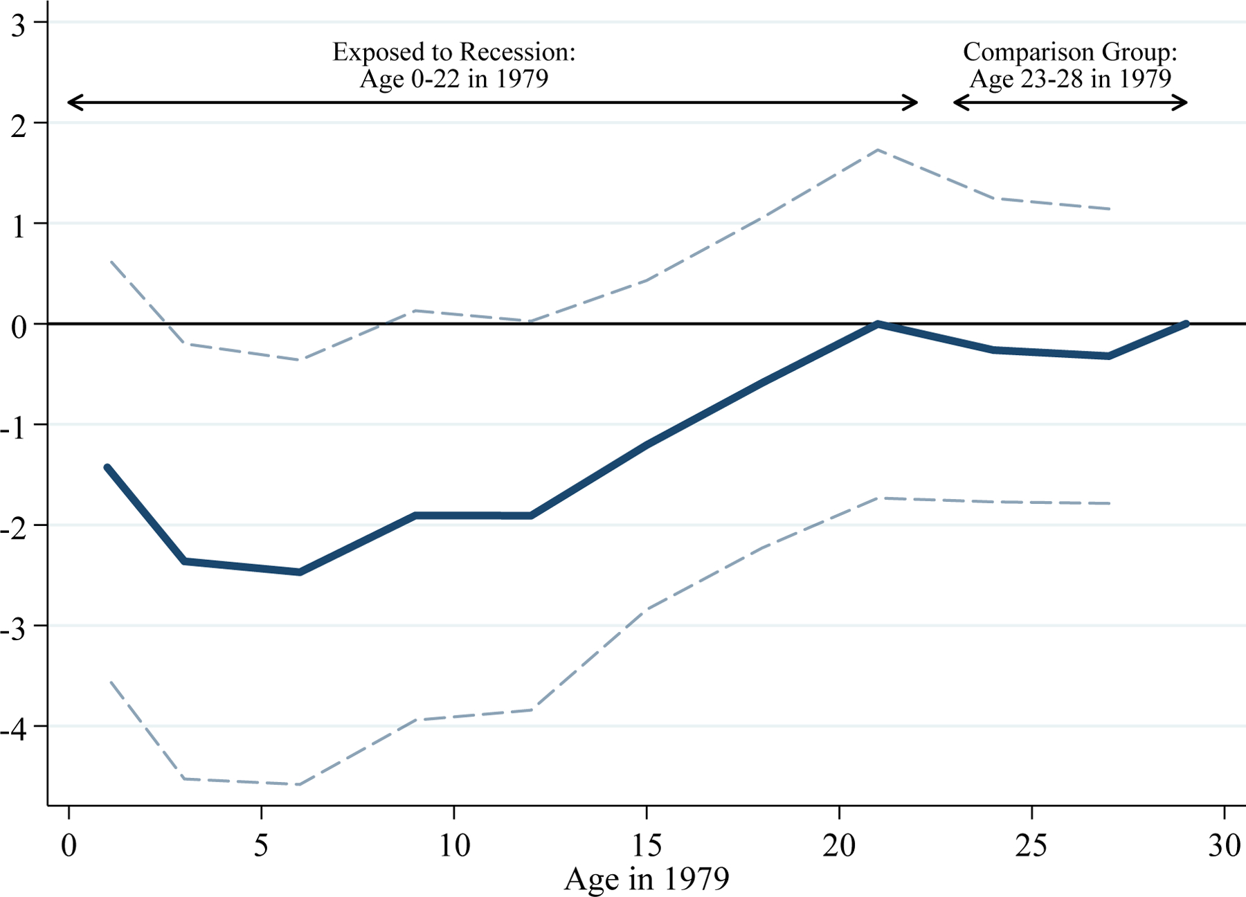
Figure 3 shows that the 1980–1982 recession reduced children’s four-year college degree attainment. The figure displays 2SLS estimates of equation (1), where I use three-year age bins to estimate πa more precisely.22 Estimates for individuals who were 23–28 years old in 1979 are small and indistinguishable from zero, indicating that the severity of the recession is not related to trends in college degree attainment for this group. Because college degree attainment is largely completed by age 23, this finding supports the validity of my empirical strategy. Negative effects emerge for individuals who were younger when the recession began, with these effects being most severe and nearly constant for individuals age 0–13 in 1979. For this group, the point estimates imply that a 10 percent decrease in earnings per capita from 1979–1982, approximately equal to one standard deviation, reduces four-year college degree attainment by about 4 percentage points, or around 13 percent of mean attainment.
Figure 3: The Long-Run Effects of the 1980–1982 Recession on Four-Year College Degree Attainment.

Notes: Figure plots estimates of the interaction between the 1979–1982 decrease in log real earnings per capita in individuals’ county of birth and indicators for age in 1979. The interaction for individuals age 29 is normalized to equal zero. The dependent variable is an indicator for four-year college degree attainment. See notes to Table 2 for details on sample and specification. To increase precision, I combine ages 0–1, 2–4, 5–7, 8–10, 11–13, 14–16, 17–19, 20–22, 23–25, and 26–28. The dashed lines are pointwise 95 percent confidence intervals based on standard errors clustered by state.
Sources: BEA Regional Economic Accounts, Census County Business Patterns, Confidential 2000–2013 Census/ACS data linked to the SSA NUMIDENT file
Figure 4 shows analogous impacts on total years of education. Estimates for individuals age 23–28 in 1979 are again small and indistinguishable from zero, providing further support for the empirical strategy. The coefficients follow a similar pattern as those in Figure 3, and are almost five times as large, providing initial evidence that most of the effects on years of education come from four-year degree attainment.23
Figure 4: The Long-Run Effects of the 1980–1982 Recession on Years of Schooling.
Notes: Figure plots estimates of the interaction between the 1979–1982 decrease in log real earnings per capita in individuals’ county of birth and indicators for age in 1979. The interaction for individuals age 29 is normalized to equal zero. The dependent variable is years of schooling. See notes to Table 2 and Figure 3 for details on sample and specification.
Sources: BEA Regional Economic Accounts, Census County Business Patterns, Confidential 2000–2013 Census/ACS data linked to the SSA NUMIDENT file
Table 2 reports estimates of long-run effects on several measures of educational attainment, grouping together individuals age 0–10 and 11–19 in 1979, while normalizing the age 20–29 coefficient to equal zero.24 There is no evidence of an effect on high school diploma or GED attainment. The point estimates for college attendance are negative, but indistinguishable from zero at conventional levels. Column 3 shows sizable and statistically significant negative effects on any college degree attainment. Columns 4 and 5 separate college degree attainment into two mutually exclusive categories: four- and two-year degrees.25 There is evidence of a decrease in four-year degree attainment, as shown in Figure 3, and no effect on two-year degree attainment. The estimates in column 6 on total years of schooling are negative; as shown in columns 1–5, these are driven by a reduction in college attendance and four-year degree attainment. For individuals age 0–10 in 1979, a 10 percent decrease in earnings per capita from 1979–1982 leads to a 2.7 percentage point (4.6 percent) decrease in college attendance, a 4.4 percentage point (10.7 percent) decrease in any college degree attainment, and a 4.7 percentage point (14.6 percent) decrease in four-year degree attainment.
Table 2:
The Long-Run Effects of the 1980–1982 Recession on Education
| Dependent variable: | ||||||
|---|---|---|---|---|---|---|
| HS/GED attainment | Any college attendance | Any college degree attainment | Four-year college degree attainment | Two-year college degree attainment | Years of schooling | |
| (1) | (2) | (3) | (4) | (5) | (6) | |
| Panel A. Interaction between 1979–1982 decrease in log real earnings per capita and age in 1979 | ||||||
| 0–10 | −0.020 (0.047) |
−0.269 (0.158) |
−0.444 (0.174) |
−0.470 (0.179) |
0.025 (0.059) |
−1.967 (0.868) |
| 11–19 | 0.055 (0.046) |
−0.141 (0.122) |
−0.297 (0.107) |
−0.286 (0.107) |
−0.010 (0.043) |
−1.065 (0.573) |
| Panel B. Average value of dependent variable in years 2000–2013, by age in 1979 | ||||||
| 0–10 | 0.936 | 0.932 | 0.414 | 0.321 | 0.093 | 13.57 |
| 11–19 | 0.932 | 0.537 | 0.380 | 0.288 | 0.093 | 13.39 |
Notes: Panel A reports estimates of the interaction between the 1979–1982 decrease in log real earnings per capita in individuals’ birth county and indicators for age in 1979. The interaction for individuals age 20–29 is normalized to equal zero. Regressions include indicators for gender-by-age at time of survey, race, birth county, age in 1979-by-birth state, and survey year, plus indicators for age in 1979 interacted with several covariates measured in individuals’ birth county: the 1950–1960, 1960–1970, and 1970–1980 change in log real median family income and log population, and the 1960 level of log population, log population density, percent urban, percent black, percent foreign, percent with a high school degree, and percent of families with income below $3,000. Regressions are estimated by 2SLS, using the predicted log employment change from 1979–1982 as an instrumental variable. Standard errors in parentheses are clustered by birth state. The sample in Panel A contains 23.5 million individuals born in the continental U.S. from 1950–1979 with a unique birth county, unique PIK, and non-allocated variables. Panel B reports average values of the dependent variables for a comparable sample from publicly available 2000 Census and 2001–2013 ACS data.
Sources: BEA Regional Economic Accounts, Census County Business Patterns, Confidential 2000–2013 Census/ACS data linked to the SSA NUMIDENT file, Publicly available 2000–2013 Census/ACS data from Ruggles et al. (2015)
These results imply that, in the absence of the recession, individuals born in counties where the recession was more severe would have been more likely to attend college and obtain a four-year degree. The larger effect on college degree attainment than attendance suggests that part of the decline in degree attainment stems from individuals not completing college because of the recession. A negative impact on college persistence could arise from a reduction in college readiness or the quality of colleges at which individuals enroll (e.g., Bound, Lovenheim and Turner, 2010). More generally, unobserved substitution patterns underlie these results. For example, individuals who would have obtained a four-year degree in the absence of the recession might have instead received a two-year degree, attended college without obtaining a degree, or not attended college. As another example, the lack of a net effect on two-year degree attainment could arise from equal-sized shifts of individuals from four-year degrees to two-year degrees (increasing two-year degree attainment) and from two-year degrees to no degree (decreasing two-year degree attainment). Economic theory and prior empirical work do not place sharp bounds on the possible adjustment margins.
Previously studied policies provide a useful comparison for understanding the size of these effects. A 10 percent decrease in earnings per capita from 1979–1982 for individuals age 0–10 in 1979 has an effect on any college degree attainment almost three times as large as the Tennessee Student/Teacher Achievement Ratio (STAR) Experiment, which randomly reduced kindergarten to grade 3 class sizes by roughly 30 percent and increased college degree attainment by 1.6 percentage points (Dynarski, Hyman and Schanzenbach, 2013). The effect of the recession on four-year college degree attainment is also larger than the STAR Experiment, which increased four-year degree attainment by 0.9 percentage points (Dynarski, Hyman and Schanzenbach, 2013), and the effect of statewide scholarship programs that fully covered tuition and fees for qualified students, which increased four-year degree attainment by 2.5 percentage points (Dynarski, 2008).
Another way to quantify these impacts is by comparing them to the cross-sectional relationship between recession severity and long-run outcomes. Appendix Table A.6 shows “first difference” estimates from a specification that does not include county fixed effects and so does not difference by age. The difference-in-differences estimates are smaller in magnitude than the first difference estimates. For four-year degree attainment, the estimated effects in Table 2 for individuals age 0–10 in 1979 are about half as large as the first difference estimates. The results also display the value of using cross-cohort variation, which facilitates the inclusion of birth county fixed effects; a purely cross-sectional research design would overstate the negative impacts of the recession on long-run outcomes.
Appendix Table A.7 presents results separately by gender and race. The impacts on educational attainment are largely similar for men and women, although there is evidence that the decline in college attendance was larger for men. The long-run effects on men and women reflect differences in the opportunity cost of education, contemporaneous labor market opportunities, and the responsiveness of boys versus girls to early life shocks (e.g., Autor et al., 2019). In terms of race, the negative impacts are concentrated among whites. The point estimates on educational attainment are positive for nonwhites, but generally insignificant. One possible explanation is that white families experienced a greater decline in wealth because they were more likely to own homes, and house values declined after the recession. Another possible explanation is the opportunity cost channel, as non-white workers experienced greater reductions in employment and wages during the recession (Bound and Holzer, 2000; Hoynes, Miller and Schaller, 2012), and this might have persisted.
5.2. Long-Run Effects on Income, Wages, and Poverty
Figure 5 shows the estimated effects of the recession on indicators for income exceeding several thresholds: $0, $2,500, $5,000, $10,000, $20,000, …, $100,000. These dependent variables (measured from 2000–2013) yield evidence on impacts throughout the income distribution. Panel A shows results for total personal income. There is little evidence that the recession affected the extensive margin, which is not surprising given the wide range of income sources included in this measure. Instead, the effects of the recession are most severe in the middle of the income distribution.26 For example, a 10 percent decrease in earnings per capita during the recession reduces the probability of earning at least $30,000 by 2 percentage points for individuals who were age 0–10 in 1979 and 1 percentage point for those age 11–19. The point estimates are more negative for the younger group than the older group at all income thresholds up to $70,000. Moving further up the income distribution, there is little effect on whether the younger group earns $80,000 or more, but there is a negative effect for the older group. A natural explanation for this pattern is that (a) the larger reduction in income for individuals age 0–10 in 1979 reflects the larger reduction in education and (b) lifecycle income growth causes more of the older group to be “at risk” of a recession-induced decrease in income in the upper part of the distribution.
Figure 5: The Long-Run Effects of the 1980–1982 Recession on Income Thresholds.
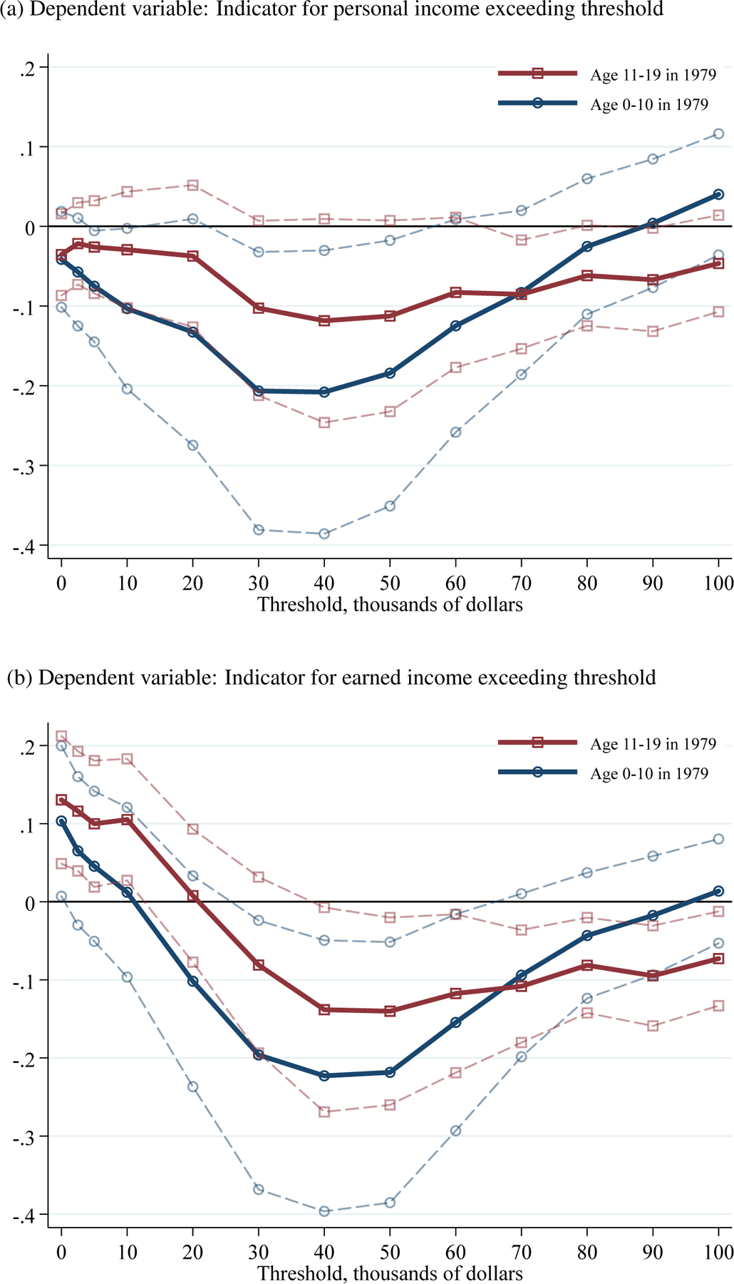
Notes: Panel A reports estimates of the interaction between the 1979–1982 decrease in log real earnings per capita in individuals’ birth county and indicators for age in 1979. The interaction for individuals age 20–29 is normalized to equal zero. The dependent variables are indicators for income exceeding thresholds $0, $2,500, $5,000, $10,000, $20,000, …, $100,000. See notes to Table 3 for details on sample and specification.
Sources: BEA Regional Economic Accounts, Census County Business Patterns, Confidential 2000–2013 Census/ACS data linked to the SSA NUMIDENT file
Panel B presents results for earned income. The pattern is similar, except the estimates are positive at low levels of income. The extensive margin effects are relatively small: a 10 percent decrease in earnings per capita leads to a 1 percentage point increase in the probability of having positive earned income for individuals who were age 0–10 in 1979. To interpret these results, recall that the identified effects are relative to those on individuals who were 20–29 years old in 1979, i.e., (π0−10 − π20−29) and (π11−19 − π20−29). If the recession led to a long-run earnings reduction of older individuals (so that π20−29 < 0, consistent with the results in Appendix Figures A.13–A.17), then the estimated effects for younger individuals are biased upwards. The similarity of the upwards shift for individuals age 0–10 and 11–19 in 1979 in Panel B suggests that the positive coefficients reflect a decrease in the probability that individuals who were age 20–29 in 1979 have positive or low levels of earnings. Because the recession led to lasting decreases in local economic activity (Appendix B), this could arise as older individuals drop out of the labor force. Many individuals with zero earnings have positive total income (including from transfers), which explains why this pattern does not appear in Panel A. This interpretation accords with summary statistics in Appendix Figure A.12, which shows that individuals who were 20–29 years old in 1979 are less likely to have positive earnings from 2000–2013 and equally likely to have positive personal and family income.
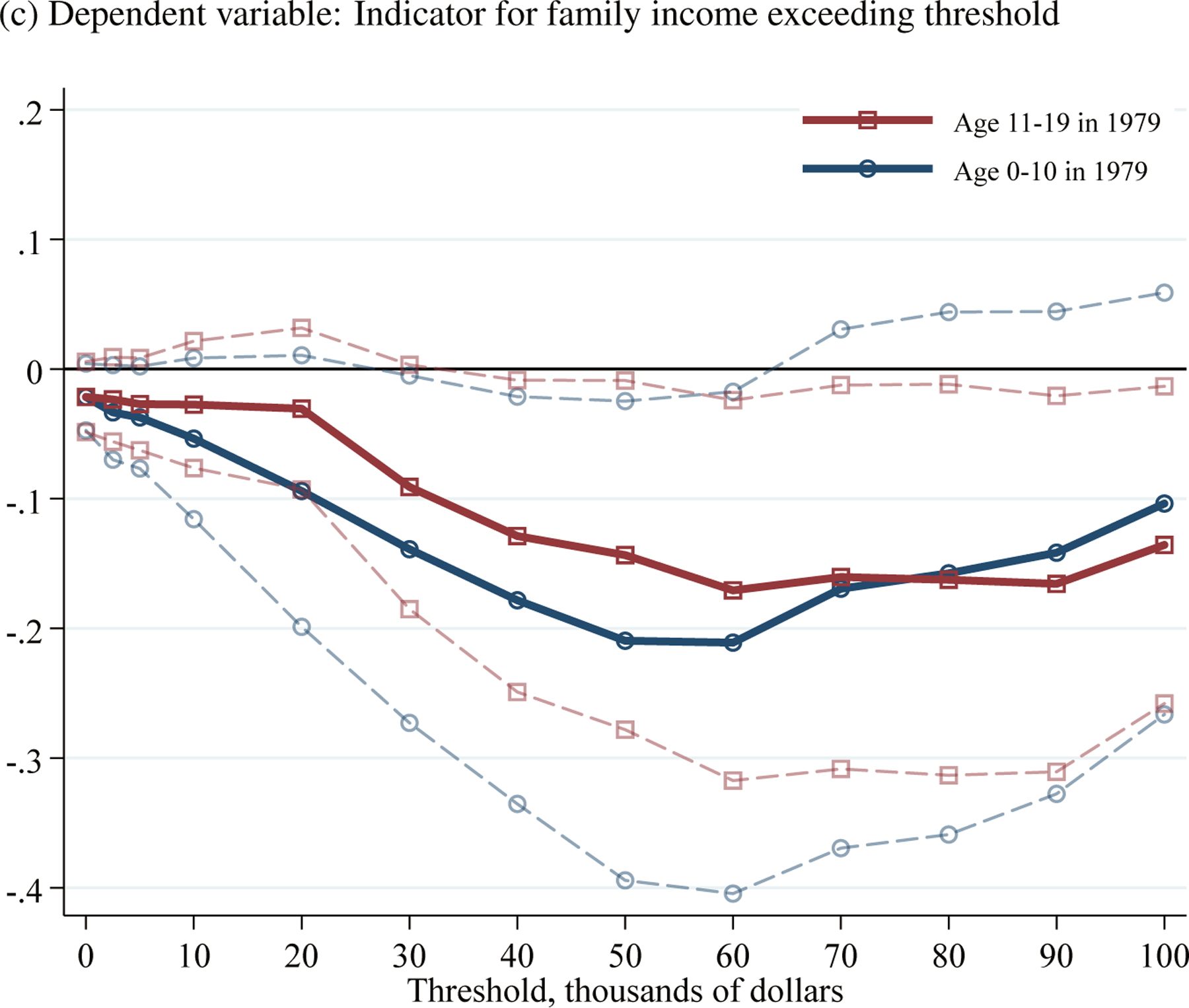
The results for family income in Panel C resemble those for personal income in Panel A. The effects extend further up the income distribution, which is not surprising because family income exceeds personal income. The results for individuals who were age 0–10 and 11–19 in 1979 are more similar, reflecting the additional heterogeneity that arises when considering families.
The estimates in Figure 5 show that the recession reduced the probability that individuals earned middle-class incomes. The ability to see these distributional effects comes at the cost of reduced precision and conciseness. To summarize the effects of the recession, I use log income and earnings as dependent variables going forward.
Table 3 shows that the recession led to long-run decreases in income and wages and increases in poverty, where these outcomes are measured from 2000–2013. For individuals age 0–10 in 1979, the estimates imply that a 10 percent decrease in earnings per capita from 1979–1982 reduces personal income by 4.5 percent ($1,900), earned income by 5.2 percent ($2,100), and hourly wages by 3.0 percent ($0.77).27 For the same group, total family income falls by 4.2 percent ($3,400), and the probability of living in poverty increases by 13.0 percent (1.6 percentage points).28 Individuals age 11–19 in 1979 experience a smaller decrease in income, a similar decrease in wages, and a smaller increase in poverty. The long-run effects of the recession on income, wages, and poverty are more severe for individuals who were children and adolescents when the recession began than for individuals who were young adults and already in the labor market. This points to the importance of human capital attainment in explaining these results. As the recession might have negatively affected individuals who were 20–29 years old in 1979, these estimates could be biased upwards (i.e., too conservative).
Table 3:
The Long-Run Effects of the 1980–1982 Recession on Income, Wages, and Poverty
| Dependent variable: | |||||
|---|---|---|---|---|---|
| Log personal income | Log earned income | Log hourly wage | Log family income | In poverty | |
| (1) | (2) | (3) | (4) | (5) | |
| Panel A. Interaction between 1979–1982 decrease in log real earnings per capita and age in 1979 | |||||
| 0–10 | −0.447 (0.158) |
−0.519 (0.166) |
−0.303 (0.125) |
−0.419 (0.173) |
0.158 (0.062) |
| 11–19 | −0.295 (0.120) |
−0.333 (0.119) |
−0.326 (0.105) |
−0.332 (0.118) |
0.070 (0.040) |
| Panel B. Average value of dependent variable in years 2000–2013, by age in 1979, in levels | |||||
| 0–10 | 42,728 | 41,004 | 25.53 | 80,971 | 0.122 |
| 11–19 | 51,325 | 48,484 | 29.80 | 94,026 | 0.103 |
Notes: See notes to Table 2. The sample in columns 1–4 contains 15.6 million individuals born from 1950–1979 in the continental U.S. with a unique birth county, unique PIK, non-allocated variables, and positive values of family income, earned income, personal income, and wage. The sample in column 5 contains 18.4 million individuals born from 1950–1979 in the continental U.S. with a unique birth county, unique PIK, and non-allocated variables. All monetary variables are in 2014 dollars.
Sources: BEA Regional Economic Accounts, Census County Business Patterns, Confidential 2000–2013 Census/ACS data linked to the SSA NUMIDENT file, Publicly available 2000–2013 Census/ACS data from Ruggles et al. (2015)
Recent work by Chetty and Hendren (2018a,b) provides a valuable comparison for understanding the size of these effects. Chetty and Hendren study what happens when children grow up in worse or better places, where neighborhood (i.e., commuting zone or county) quality is fixed over time and measured by the income in adulthood of permanent residents. As a result, Chetty and Hendren’s neighborhood quality measure reflects many determinants of long-run outcomes be sides local economic conditions. Nonetheless, the effects of the recession are sizable relative to Chetty and Hendren’s measure: for individuals age 0–10 in 1979, a 1 standard deviation increase in recession severity has similar effects on family income as a 0.5 standard deviation decrease in Chetty and Hendren’s county quality measure throughout childhood.29
The age profiles in Table 3 are similar to those in Table 2, as the effects generally are more severe for individuals age 0–10 in 1979.30 The impacts on labor market outcomes for the younger group could be attenuated by life-cycle bias (Haider and Solon, 2006). In particular, the effect of the recession on income and wages early in an individual’s career could be biased upwards relative to the lifetime effect. As a result, I likely understate the size of the lifetime effect for individuals who were younger when the recession began.31
To explore the role of education in these results, I calculate the implied effects of the recession on income and wages based on the estimated effects on education and OLS estimates of the returns to high school/GED attainment, college attendance, two-year degree attainment, and four-year degree attainment.32 Column 1 of Table 4 reports the estimates from Table 3 for reference. The estimates in column 2 show that the implied effects via education can account for much of the estimated magnitudes: the predicted effects are 41–85 percent as large as the actual effects. This evidence is simply suggestive, as the OLS estimates might differ from the causal returns to education for this population because of omitted variables bias or heterogeneity in the returns to schooling.
Table 4:
The Long-Run Effects of the 1980–1982 Recession on Income and Wages, Examining the Role of Education and Commuting Zone of Residence
| Relative Effect | |||||
|---|---|---|---|---|---|
| Estimated effect on dependent variable | Implied by effects on education | Estimated effect on mean in CZ of residence | Education | CZ of residence | |
| (1) | (2) | (3) | (4) | (5) | |
| Interaction between 1979–1982 decrease in log real earnings per capita and age in 1979 | |||||
| Panel A. Dependent variable: Log personal income | |||||
| 0–10 | −0.447 (0.158) |
−0.317 (0.164) |
−0.254 (0.084) |
0.710 | 0.568 |
| 11–19 | −0.295 (0.120) |
−0.153 (0.115) |
−0.149 (0.053) |
0.520 | 0.504 |
| Panel B. Dependent variable: Log hourly wage | |||||
| 0–10 | −0.303 (0.125) |
−0.259 (0.124) |
−0.204 (0.073) |
0.853 | 0.672 |
| 11–19 | −0.326 (0.105) |
−0.138 (0.084) |
−0.145 (0.047) |
0.424 | 0.444 |
| Panel C. Dependent variable: Log family income | |||||
| 0–10 | −0.419 (0.173) |
−0.289 (0.150) |
−0.250 (0.085) |
0.689 | 0.596 |
| 11–19 | −0.332 (0.118) |
−0.136 (0.106) |
−0.157 (0.052) |
0.411 | 0.472 |
Notes: Column 1 reports the estimated effect on the dependent variable from Table 3. Column 2 reports the implied effect based on the estimates in Table 2 (columns 1, 2, 4, and 5) and OLS regressions of income and wages on these measures of education plus indicators for gender-by-age, race, and year. In column 3, the dependent variable is mean log income or wage of all workers age 25–64 who live in individuals’ CZ of residence. Column 4 equals the ratio of column 2 to column 1, and column 5 equals the ratio of column 3 to column 1.
Sources: BEA Regional Economic Accounts, Census County Business Patterns, Confidential 2000–2013 Census/ACS data linked to the SSA NUMIDENT file, Publicly available 2000–2013 Census/ACS data from Ruggles et al. (2015)
The negative effects on income and wages also might arise from individuals’ tendency to live and work near their place of birth, which experienced a persistent decrease in local economic activity following the 1980–1982 recession. To examine this, I estimate regressions in which the dependent variable is the mean log income or wage of all workers age 25–64 who live in the individual’s 2000–2013 commuting zone of residence. The estimates are in column 3 of Table 4. Interestingly, the pattern of coefficients is similar to the estimated impacts on education and income. This implies that individuals age 0–10 in 1979 live in commuting zones with lower mean income than individuals age 11–19 in 1979. The estimated impacts on mean income in individuals’ CZ of residence are 44–67 percent as large as the impacts on individuals’ income. Consequently, location also appears to be an important mediating factor. In interpreting these results, it is important to note that individuals’ location depends partly on their educational attainment (Wozniak, 2010; Malamud and Wozniak, 2012).
Appendix Table A.8 displays the cross-sectional relationship between recession severity and income in adulthood. For earned income, the difference-in-difference estimates in Table 3 for 0–10 year olds are about one-third as large as the first difference estimates. Although we cannot interpret the first difference estimates on 20–29 year olds as causal (e.g., because of the education differentials apparent in Table A.6), it is reassuring that the difference-in-difference estimates are of a reasonable order of magnitude. Appendix Table A.9 shows heterogeneity in the impacts by gender and race; these are largely as expected, given the heterogeneity in the impacts on education.
5.3. Evidence Supporting the Empirical Strategy and Robustness
Several pieces of evidence suggest that these long-run effects are due to the recession, as opposed to some confounding variable. Most importantly, the falsification tests in Figures 3 and 4 show a lack of pre-trends in educational attainment. Furthermore, my empirical strategy exploits sudden changes in local economic activity driven by the interaction of pre-existing industrial specialization and aggregate employment changes that emerged during the 1980–1982 recession. This research design mitigates many potential concerns about selective migration or fertility before 1980. As discussed in Appendix B, the industrial specialization that led to severe earnings and employment losses during the 1980–1982 recession is uncorrelated with counties’ median family income growth from 1970–1980 and correlated with higher income growth from 1950–1970. My regressions control flexibly for pre-recession changes in log median family income and other county-level covariates. Furthermore, there is little correlation between the predicted log employment change from 1979–1982 and the severity of other recessions from 1973–2009, Japanese import competition from 1970–1990, or Chinese import competition from 1991–2007.33
Appendix F describes results from birth certificate data that provide additional evidence on the validity of my empirical strategy. Most importantly, I find no evidence that the evolution of infant mortality from 1950–1979 is correlated with the severity of the 1980–1982 recession. There is also no evidence that my results are driven by a decrease in maternal education or infant birth weight. These results strongly rule out the possibility that my estimates simply reflect changes in infant health. Appendix G describes additional robustness tests, all of which support my conclusions about the long-run effects of the 1980–1982 recession.
5.4. Mechanisms
The age profile in Figure 3 informs the mechanisms underlying these long-run effects. As discussed in Section 3, negative long-run effects on children could stem from a decrease in childhood human capital development or a decrease in parental resources to finance college in the presence of credit constraints. In principle, a decrease in parental resources to finance college also could affect teenagers and individuals already enrolled in college. However, I estimate small and statistically insignificant effects for individuals age 14–22 in 1979, which suggests that the short-term decrease in parental resources plays a minor role. Table 2 shows that the negative effects of the recession are concentrated at higher levels of educational attainment, for which childhood human capital and parental resources seem to have the largest impacts (Belley and Lochner, 2007; Bailey and Dynarski, 2011).
Both human capital development during childhood and parental resources to finance college could fall because of a decline in parental earnings. While my data do not contain information on parents’ labor market outcomes, estimates of the long-run effects of parental job displacement provide a benchmark. If job loss generated all of the county-level decrease in earnings per capita from 1979–1982 and the recession only affected children whose parents lost a job, then previous work suggests that a 10 percent decrease in earnings per capita would decrease college attendance by 0.5 percentage points (Hilger, 2016), 1.5 percentage points (Page, Stevens and Lindo, 2007), or 10 percentage points (Coelli, 2011).34 These studies typically focus on children who are teenagers at the time of job loss. For this group, Table 2 implies that a 10 percent decrease in earnings per capita leads to an imprecisely estimated 1.4 percentage point decrease in college attendance. This point estimate lies within the wide range predicted by past work, suggesting that parental job loss could explain the effects of the recession on college attendance. A similar conclusion holds when looking at the long-run effects of the recession on income.35 However, these conclusions are tempered by the wide range of estimates from the parental job displacement literature.
Human capital development during childhood could fall because of a decline in community investments. While I cannot measure most forms of community investment, like neighborhood or school quality, data on local government expenditures are available. As described in Appendix H, expenditures per capita fell starting in the early 1990s in counties with a more severe recession, but there is little evidence of a change before then. The decline in expenditures is driven by spending on welfare and health, and not education. These results imply that, in principle, the decrease in expenditures could contribute to the effects of the recession on individuals born in the 1970s, but not the effects on individuals born in the 1960s.
Other mechanisms could shape the long-run effects. The opportunity cost channel predicts positive effects of the recession on educational attainment. Given the persistence of the decline in local economic activity, this channel could influence children and adolescents, in addition to older individuals making contemporaneous enrollment decisions. For children and adolescents, my results indicate that opportunity cost is dominated by the mechanisms that reduce educational attainment.36
Previous studies also find that individuals who graduate from college during a recession experience a lasting decline in earnings and wages relative to graduates who enter a stronger labor market, partly due to working at lower paying employers (Kahn, 2010; Oreopoulos, von Wachter and Heisz, 2012; Altonji, Kahn and Speer, 2016). This channel could explain some of the decrease in income and wages.37
5.5. Potentially Mitigating Policies
Finally, I examine policies that might have mitigated the recession’s long-run effects. To do so, I estimate interactions between the severity of the recession and features of individuals’ birth state. This augments my baseline specification in equation (1), which includes birth state-by-birth year fixed effects. I focus on four-year college degree attainment because of its importance for individuals and the economy.
States might have mitigated the recession’s long-run effects with more generous transfer programs that insured families and communities against earnings declines. In measuring states’ transfer generosity, I control for economic and demographic characteristics that could relate mechanically to higher transfers by regressing, at the state-level, log transfers per capita in 1970 on log median family income in 1969 and the share of the 1970 population that is black, female, foreign born, urban, a high school graduate, a college graduate, and age 5–19, 20–64, and 65 and above.38 Columns 1 and 2 of Table 5 divide the sample into states with less and more generous transfers per capita using the residuals from this regression. The point estimates suggest that the effects of the recession are more severe in states with more generous transfers, but the estimates are not statistically distinguishable (p = 0.52). There is little evidence that states with more generous transfer programs mitigated the recession’s effects.
Table 5:
The Long-Run Effects of the 1980–1982 Recession on Four-Year College Degree Attainment, Potentially Mitigating Policies
| Policy: | State transfer generosity | State higher education funding | State transfer progressivity | |||
|---|---|---|---|---|---|---|
| Less generous | More generous | Less generous | More generous | Less progressive | More progressive | |
| (1) | (2) | (3) | (4) | (5) | (6) | |
| Interaction between 1979–1982 decrease in log real earnings per capita and age in 1979 | ||||||
| 0–10 | −0.382 (0.174) |
−0.536 (0.283) |
−0.678 (0.280) |
−0.312 (0.177) |
−0.360 (0.207) |
−0.541 (0.231) |
| 11–19 | −0.185 (0.098) |
−0.366 (0.175) |
−0.335 (0.173) |
−0.244 (0.121) |
−0.161 (0.166) |
−0.372 (0.132) |
| p-value, equal effects | 0.516 | 0.204 | 0.529 | |||
Notes: See notes to Table 2. Each column reports the results of a separate 2SLS regression. The p-value is for the null hypothesis that the effects of the recession are equal across columns. States with less generous transfers are those with below-median log transfers per capita in 1970, conditional on log median family income in 1969 and the share of the 1970 population that is black, female, foreign born, urban, a high school graduate, a college graduate, and age 5–19, 20–64, and 65 and above. States with less generous higher education funding are those with below-median log higher education appropriations per capita in 1970, conditional on the same demographic and economic covariates. States with less progressive transfers are those with an above-median slope coefficient from a county-level regression of log transfers per capita on log median family income in 1970 and the same demographic and economic covariates.
Sources: BEA Regional Economic Accounts, Census County Business Patterns, Confidential 2000–2013 Census/ACS data linked to the SSA NUMIDENT file, Census County Data Book, Grapevine Appropriations Data
To examine whether overall transfer generosity masks effects of more targeted transfers, I use Grapevine data to divide the sample into states with higher versus lower per capita appropriations to higher education in 1970, conditional on the same economic and demographic characteristics. The point estimates in columns 3 and 4 suggest that the effect of the recession on four-year degree attainment of individuals age 0–10 in 1979 is over 50 percent smaller in states with more generous higher education transfers. However, the estimates again are not statistically distinguishable (p = 0.20).39
Another possibility is that states which transfer more money to poor counties mitigated the long-run effects of the recession. To characterize states’ transfer progressivity, I regress log transfers per capita in 1970 on log median family income in 1969, state fixed effects, and the previously listed control variables, with the dependent and explanatory variables measured at the county-level. Columns 5 and 6 present results from dividing states into two groups using the state-specific slope coefficient on log median family income.40 The effects of the recession are considerably less severe in states with more progressive transfers. However, the estimates are not statistically distinguishable (p = 0.53), providing little evidence that states with more progressive transfers mitigated the recession’s effects. Ultimately, more research is needed to understand whether any policies mitigated the recession’s long-run effects.
A separate possible mitigating factor is the post-recession recovery. To examine this, I estimate regressions that include the decrease in log real earnings per capita from 1979–1982 and 1982–1992. As instrumental variables, I use the predicted log employment change from 1979–1982 and 1982–1992, based on a county’s 1976 industrial structure. The results in Appendix Table A.19 show that, conditional on the extent of post-recession recovery, there are sizable negative effects of the earnings decrease during the recession (similar to the estimates in Table 2).41 At the same time, a relative decrease in earnings per capita after the recession also leads to reductions in education; this implies that stronger post-recession growth had the potential to mitigate some of the recession’s effects. Consequently, policies that promote local economic growth or encourage families to migrate to stronger local labor markets could be effective at mitigating the recession’s long-run effects.
6. Conclusion: The Long-Run Effects of Recessions
This paper provides new evidence on the long-run effects of recessions on education and income. Using confidential Census data linked to county of birth and a generalized difference-in-differences framework, I estimate the long-run effects of the 1980–1982 recession on individuals who were children, adolescents, and young adults when the recession began. I find that the recession generated sizable long-run reductions in education and income. For individuals age 0–10 in 1979, a 10 percent decrease in earnings per capita from 1979–1982 in their county of birth leads to a 4.7 percentage point (14.6 percent) decrease in four-year college degree attainment, a $2,100 (5.2 percent) decrease in earned income, and a 1.6 percentage point (13.0 percent) increase in the probability of living in poverty as of 2000–2013. The negative effects on college graduation are most severe and essentially constant for individuals age 0–13 in 1979, and small and statistically insignificant for individuals age 14–22, which suggests that the underlying mechanisms are a decline in childhood human capital or a long-term decline in parental resources to pay for college.
The magnitude of these estimates and the large number of affected individuals suggest that the 1980–1982 recession depresses aggregate economic output today. Table 6 reports back of the envelope calculations that scale my difference-in-differences estimates by the 70 million individuals born in the U.S. from 1960–1979. In particular, I calculate the aggregate effect of the recession for individuals who were age a in 1979 as , where Na,c is the number of individuals born in county c who would have been age a in 1979, is the observed decrease in log real earnings per capita from 1979–1982, is the counterfactual decrease, and is the difference-in-differences estimate from equation (1) after adjusting for measurement error. If I assume that all counties would have experienced no change in real earnings per capita in the absence of the recession, these calculations imply that the recession led to 1.3 million fewer four-year college graduates, $66 billion less earned income per year, and 403,000 more adults living in poverty each year. If I instead assume that all counties would have experienced the average growth in real earnings per capita from 1969–1979 of 1.8 percent per year, these calculations suggest that the recession led to 2.8 million fewer four-year college graduates, $139 billion less earned income per year, and 850,000 more adults living in poverty each year. These numbers amount to 2–4 percent of the stock of college-educated adults in 2015, 0.4–0.8 percent of GDP in 2015 and 0.7–1.5 percent of GDP in 1979, and 1–2 percent of the number of individuals in poverty in 2015.42 While these simple calculations could understate or overstate the true aggregate effects, they suggest that the 1980–1982 recession considerably reduces aggregate economic output and welfare today.43
Table 6:
Back of the Envelope Calculations of the Aggregate Long-Run Effects of the 1980–1982 Recession
| Counterfactual 1: No real earnings per capita growth, 1979–1982 | Counterfactual 2: Trend real earnings per capita growth, 1979–1982 | ||||||
|---|---|---|---|---|---|---|---|
| Number of births, millions | Four-year college graduates | Earned income, billions $ | Adults living in poverty | Four-year college graduates | Earned income, billions $ | Adults living in poverty | |
| (1) | (2) | (3) | (4) | (5) | (6) | (7) | |
| Age in 1979 | |||||||
| 0–10 | 36.0 | −844,000 | −38.2 | 284,000 | −1,779,000 | −80.6 | 598,000 |
| 11–19 | 34.1 | −489,000 | −27.6 | 120,000 | −1,029,000 | −58.1 | 252,000 |
| 0–19 | 70.2 | −1,333,000 | −65.8 | 403,000 | −2,808,000 | −138.6 | 850,000 |
Notes: Table displays back of the envelope calculations of the aggregate long-run effects of the 1980–1982 recession. For individuals who were a years old in 1979, I calculate these as , where Na,c is the number of births of individuals residing in county c net of infant mortality, is the observed decrease in log real earnings per capita from 1979–1982 in county c, is the counterfactual decrease in log real earnings per capita, and is the difference-in-differences estimate after adjusting for measurement error. In counterfactual 1, I set and in counterfactual 2, , which corresponds to the average annual growth in earnings per capita from 1969–1979 of 1.84 percent. Column 1 reports the total number of births for each age group, net of infant mortality (Σc Na,c). Columns 2 and 5 use difference-in-differences estimates from column 4 of Table 2. Columns 3 and 6 use estimates from column 2 of Table 3. Columns 4 and 7 use estimates from column 5 of Table 3. Numbers are rounded.
Sources: BEA Regional Economic Accounts, Census County Business Patterns, Confidential 2000–2013 Census/ACS data linked to the SSA NUMIDENT file, Birth and infant mortality data from Bailey et al. (2018)
This paper shows that the 1980–1982 recession persistently decreased earnings per capita in negatively affected counties, and children and adolescents born in these counties have less education and income as adults. While I have not examined whether other recessions have similar long-run effects, Figure 6 provides reason for concern: every U.S. recession since 1973 has led to a persistent relative decrease in earnings per capita in negatively affected counties.44 This novel stylized fact indicates that the 1980–1982 recession is not unique in its persistent effects on county-level earnings per capita, which suggests that it might not be unique in its long-run effects on human capital.
Figure 6: Percent Difference in Mean Real Earnings per Capita between Counties with More versus Less Severe Recession.

Notes: Figure displays the difference in population-weighted mean real earnings per capita between counties with a more versus less severe recession, as a share of the less severe recession mean. Separately for each recession, I define counties with a more severe recession as those with an above median decrease in log real earnings per capita from 1973–1975, 1979–1982, 1989–1991, 2000–2002, and 2007–2010. I calculate the medians using population weights in the pre-recession years. Each line is normalized to equal zero in the pre-recession year via a parallel shift upwards or downwards. Sample contains 3,076 counties in the continental U.S.
Source: BEA Regional Economic Accounts
I find little evidence that states with more generous or more progressive transfer systems mitigated the 1980–1982 recession’s long-run effects. An open question left for future work is which policies, if any, temper the declines in human capital attainment. The importance of understanding these effects is underlined by the possibility that similar long-run effects could arise from other shocks leading to persistent declines in local economic activity, such as Chinese import competition (Autor, Dorn and Hanson, 2013).
Acknowledgments
I thank the editor (Alexandre Mas), two anonymous referees, Martha Bailey, Dominick Bartelme, Alexander Bartik, Jacob Bastian, Hoyt Bleakley, John Bound, Varanya Chaubey, Austin Davis, John DiNardo, Andrew Goodman-Bacon, Alan Griffith, Morgan Henderson, Jessamyn Schaller, Michael Mueller-Smith, Gary Solon, Jeffrey Smith, Isaac Sorkin, Evan Taylor, Till von Wachter, Reed Walker, Justin Wolfers, Mike Zabek, and numerous seminar and conference participants for helpful comments. Thanks to J. Clint Carter and Margaret Levenstein for help accessing confidential Census Bureau data, and to Mary Kate Batistich and Timothy Bond for sharing data. This research was supported in part by the Michigan Institute for Teaching and Research in Economics, plus an NICHD training grant (T32 HD007339) and an NICHD center grant (R24 HD041028) to the Population Studies Center at the University of Michigan. Any opinions and conclusions expressed herein are those of the author and do not necessarily represent the views of the U.S. Census Bureau. All results have been reviewed to ensure that no confidential information is disclosed.
Appendices - For Online Publication
A. Matching NUMIDENT Data to Counties
This section describes the procedure used to match the Social Security Administration NUMIDENT file to FIPS county codes. The procedure described here was developed alongside Martha Bailey, Evan Taylor, and Reed Walker. Researchers with access to confidential Census data can read a technical memo with more information on this procedure and will be able to access the code and output from this procedure (Taylor, Stuart and Bailey, 2016).
We seek to match information on individuals’ place of birth to county FIPS codes. The NUMIDENT file, which draws on Social Security card applications, contains a 12-character string identifying the place of birth (city and/or county) and a 2-character string identifying the state of birth postal code. We identify a set of target locations using U.S. Geological Survey data on current and historical locations from the Geographic Names Information System (GNIS).45 GNIS data contain place names and county FIPS codes.
Several challenges prevent exact, unique matching of the NUMIDENT 12-character strings to GNIS counties. First, some place names in a state are indistinguishable with only 12 characters.46 Second, place names are frequently misspelled. Third, the place of birth string sometimes contains acronyms and abbreviations, such as “Mnpls” for Minneapolis. Fourth, some NUMIDENT records contain the wrong postal code for their state of birth (e.g., “Anchorage, AL”).
Our algorithm yields four broad categories of matches. Each step proceeds sequentially and only applies to NUMIDENT strings not previously matched. In a preliminary processing step, we correct for common acronyms and abbreviations by hand for any string that occurs more than 50 times in the NUMIDENT data for the 1950–1985 birth cohorts. First, we obtain exact matches for correctly spelled place names that can be uniquely identified in a birth state with 12 characters. Second, we obtain “duplicate” matches for correctly spelled place names that can, in principle, be identified uniquely in 12 characters. We assign individuals to a single birth county if at least 75 percent of the exact matches are to a single county, and we assign multiple birth counties otherwise.47 Third, we use hand matches from Isen, Rossin-Slater and Walker (2017), described in their Appendix C. Fourth, we use probabilistic matching algorithms.48 Finally, we hand check all strings that are matched in the probabilistic step, disagree with the match found in the Isen, Rossin-Slater and Walker (2017) algorithm but were not hand checked by them, and have at least 50 occurrences in the NUMIDENT file for the 1950–1985 cohorts.
Appendix Table A.1 summarizes match rates for individuals observed in the 2000 Census and 2001–2013 ACS. I limit the sample to individuals who were born from 1950–1980 and were age 25–64 at the time of the survey. I also limit the sample to individuals with non-allocated values of gender, age, race, and state of birth, and who report being born in the U.S on the census survey. 95.9 percent of the sample has a non-missing protected identification key (PIK), which is the anonymous identifier used to link Census/ACS and SSA data. Of these individuals, 99.6 percent have a PIK that is not duplicated within a survey year. We identify a unique birth county for 93.6 percent of the individuals with non-duplicated PIKs. Ultimately, these restrictions leave 89.4 percent of the initial sample. The majority of matches, 80.4 percent, are exact matches, while 11.0 percent are duplicates, 5.1 percent are matched probabilistically, and 3.5 percent are hand matches.
B. Recession Severity and the Evolution of Median Family Income from 1950–2010
The BEA earnings data used in Figure 2 are only available starting in 1969. In this section, I examine the relationship between the evolution of median family income from 1950–2010 and the severity of the recession predicted by pre-existing industrial specialization.
I examine the evolution of median family income from 1950–2010 by estimating the regression
| (A.1) |
where yc,t is log real median family income in county c and year t.49 The key explanatory variable is the 1979–1982 decrease in log real earnings per capita, . In some specifications, xc,t contains time-varying covariates described below. The regression includes county fixed effects, γc, to absorb time-invariant differences across counties and state by year fixed effects, θs(c),t, which I include in equation (1) when estimating long-run effects on individuals. I normalize α1980 = 0, so that (α1950, α1960, α1970) describe how the pre-recession evolution of log median family income is correlated with the severity of the 1980–1982 recession, and (α1990, α2000, α2010) describe the post-recession evolution. I estimate equation (A.1) with two-stage least squares (2SLS), where the instrument for is the predicted log employment change, . I cluster standard errors by state, and I initially exclude the 526 counties with at least 5 percent of 1976 employment in the mining sector, which includes oil and gas extraction, to minimize the countercyclical boom-bust cycle in this sector. These high-mining counties account for only 6 percent of U.S. population, but receive considerably more weight in 2SLS estimates of equation (A.1) because pre-existing industrial specialization strongly influences their earnings per capita.
The estimates of αt in Appendix Figure A.2 characterize the 1980–1982 recession as a reversal of post-war fortune: counties with a more severe recession saw greater median family income growth from 1950–1970. This pattern arises from estimates of model 1, which contains county and state-by-year fixed effects but no other covariates. Model 2, which adds interactions between year and the 1950–1970 log median family income change and the other county-level covariates included in equation (1) (see also the figure notes), eliminates this pre-trend. County-level controls have no effect on the 1990 coefficient, but lower the 2000 and 2010 coefficients somewhat, indicating that counties with a more severe recession have other covariates associated with higher earnings in these years. Finally, model 3 controls for the 1950–1960, 1960–1970, and 1970–1980 change in log median family income, mechanically eliminating any pre-trend; this model includes the same covariates as my main specification of equation (1). The estimated coefficients and confidence intervals for 1990, 2000, and 2010 are essentially identical. The model 3 estimates imply that a 10 percent decrease in earnings per capita from 1979–1982 led to an 8.8 percent decrease in real median family income in 1990, a 13.3 percent decrease in 2000, and a 22.9 percent decrease in 2010.50
C. Imputing Employment in County Business Patterns Data
This section describes how I impute employment in Census CBP data. CBP data always report establishment counts by county, industry, and establishment size, but frequently suppress employment at the county by industry level. From 1974-forward, the establishment size groups are 1–4, 5–9, 10–19, 20–49, 50–99, 100–249, 250–499, 500–999, 1000–1499, 1500–2499, 2500–4999, and 5000 or more employees.
I impute employment at the county-by-industry level using establishment counts and nation-wide information on employment by establishment size. For establishments with fewer than 1000 employees, I impute employment as the number of establishments times average 1977 employment in the establishment size group, where the average comes from nationwide data across all industries.
Nationwide CBP data report total employment among establishments with at least 1000 employees, but not by establishment size group. To impute employment for these large establishments, I assume that employment follows a log normal distribution, with mean μ and standard deviation σ, and estimate (μ, σ) using the generalized method of moments (GMM), as in Holmes and Stevens (2002). I estimate (μ, σ) using the following four moments:
| (A.2) |
| (A.3) |
| (A.4) |
| (A.5) |
where p1 is the share of establishments (with at least 1000 employees) with 1000–1499 employees, p2 is the share with 1500–2499 employees, p3 is the share with 2500–4999 employees, Φ(·) is the standard normal CDF, and E[y] is average employment among establishments with at least 1000 employees.
I use equations (A.2)–(A.5) to estimate (μ, σ) with GMM, using the identity matrix as the weighting matrix. Using 1977 data across all industries in the U.S., there are 1947 establishments with 1000–1499 employees, 1202 with 1500–2499 employees, 678 with 2500–4999 employees, and 275 with 5000 or more employees. Total employment among these establishments is 9,442,953. Consequently, , , and . The GMM estimates are and . Standard facts about the log-normal distribution imply that the imputed means for the four establishment size groups are 1247, 1952, 3414, and 7055.51
D. Addressing Measurement Error in Recession Exposure
This section describes measurement error that arises because some individuals’ county of residence in 1979, which is the ideal variable for measuring recession exposure, differs from their county of birth, which is all I observe. I show that this measurement error attenuates estimates of πa in equation (1), and I quantify the size of this attenuation.
For reference, I repeat equation (1), which is the feasible regression of interest:
| (A.6) |
The explanatory variable of interest in equation (A.6) is , the change in log earnings per capita from 1979–1982 in birth county c. Let be the change in log earnings per capita from 1979–1982 in the county where individual i resided in 1979. This variable more accurately measures exposure to the recession, but is unobserved. If I observed county of residence in 1979, the regression of interest would be
| (A.7) |
True recession exposure, , and observed recession exposure, , are connected through an auxiliary measurement error equation,
| (A.8) |
Equation (A.8) does not contain birth county fixed effects because the attenuation bias arises from cross-county variation for each cohort. By definition, vi,a,c,t is uncorrelated with the variables in Equation (A.8).
To analyze the consequences of measurement error, I use the Frisch-Waugh-Lovell theorem (Frisch and Waugh, 1933; Lovell, 1963). I first partial out xi,a,c,t, age in 1979-by-birth state fixed effects, and survey year fixed effects from equations (A.6)–(A.8). Let M1z represent the resulting residual for some vector z, where M1 is the “annihilator matrix.” Equations (A.6)–(A.8) can then be written:
| (A.9) |
| (A.10) |
| (A.11) |
Plugging equation (A.11) into (A.10) leads to:
| (A.12) |
If is orthogonal to both , conditional on the covariates in equation (A.7), and the measurement error, vi,a,c,t, then equations (A.9) and (A.12) imply that plim , where is the OLS estimate from equation (A.6).52 Analogous conditions hold for 2SLS estimates. Consequently, the estimated effects of the recession will be attenuated if λa ∈ (0. 1), and I can eliminate this attenuation bias with an estimate of λa.53
To quantify the extent of attenuation, the ideal data set is the 1980 Census linked to the NUMIDENT. Unfortunately, these files are not currently linked. Instead, I estimate λa using two data sets that provide valuable, but imperfect, information. First, I use 2000–2013 Census/ACS data for individuals born from 1970–2013 who are ages 0 to 29 at the time of the survey. These data contain county of birth from the NUMIDENT, like the data I use to estimate the long-run effects of the 1980–1982 recession, and county of residence at the time of the survey. Because they measure the relationship between county of birth and county of residence after the 1980–1982 recession, they might not accurately characterize measurement error if migration patterns have changed over time. To address this concern, I use confidential Panel Study of Income Dynamics (PSID) data. PSID data allow me to estimate λa for individuals born from 1968–1979 and observed in 1979, but they only contain information on county of residence. I limit the PSID sample to individuals who are first observed before age 3 to make early life county of residence a better proxy for county of birth.
As seen in Appendix Figure A.4, point estimates of λa from Census/ACS data range from 0.75 for 0 year olds to 0.40 for 29 year olds. Point estimates from PSID data display a similar age profile, but are larger because county of residence is more strongly related to county of residence in early life than county of birth. Appendix Figure A.4 clearly suggests attenuation due to measurement error.
To adjust for attenuation, I use the Census/ACS data because they contain more comparable information on place of birth. The validity of this adjustment depends on two assumptions. First, I assume that unobserved measurement error, vi,a,c,t, is uncorrelated with unobserved determinants of long-run outcomes, , conditional on the covariates in equation (A.6). For example, this rules out the possibility that parents of young children with high anticipated the recession and moved to less severe recession counties before 1980. The suddenness of the changes in local economic activity that emerged during the recession support this assumption. In addition, there is no significant relationship between the severity of the 1980–1982 recession and migration from 1975 to 1980 in publicly available Census data. Second, I assume that estimates of λa for individuals born from 1970–2013 accurately characterize the measurement error relationship for individuals born from 1950–1979. Support for this assumption comes from the fact that estimates of λa are stable across the 1968–2013 birth cohorts in the PSID, as shown in Appendix Table A.2. Appendix Figure A.5 shows that migration rates are remarkably stable across the 1968–2013 birth cohorts in the PSID.
Appendix Figure A.6 shows the consequences of adjusting the effects of the recession on four-year college degree attainment for attenuation bias. The adjusted effects are larger in magnitude, but they lie within the 95 percent confidence interval of the unadjusted estimates. Appendix Figures A.7–A.11 present the measurement error adjustments for other educational outcomes.
For the tables, I construct equally-weighted averages of the λa coefficients across ages. The resulting averages are 0.673 (standard error: 0.021) for 0–10 year olds and 0.573 (0.016) for 11–19 year olds. Not surprisingly, they are even more precisely estimated than the results in Appendix Figure A.4, which are already quite precise.
To account for uncertainty due to estimation of the measurement error coefficients, I construct standard errors of the adjusted estimates using the delta method. In particular, the variance of the measurement error adjusted estimate is
| (A.13) |
The first part of this variance is the mechanical effect that arises from rescaling the estimates by the measurement error coefficient, λa. The second part is the additional variance that arises from estimating the measurement error model. It is instructive to calculate these components separately. For the effect of the recession on four-year college degree attainment of individuals who were age 0–10 in 1979, the adjusted standard error in column 4 of Table 2 is 0.179. The variance is:
| (A.14) |
Uncertainty due to estimation of the measurement error model has a negligible effect on the variance of the adjusted estimate. The variance of the adjusted estimate exceeds that of the unadjusted estimate, but this is almost entirely due to the first term, which rescales the unadjusted variance by . This is because the measurement error parameters are estimated very precisely.
E. The Long-Run Effects of the 1980–1982 Recession: First Stage, Reduced-Form, and OLS Estimates
Appendix Table A.3 reports first stage estimates. Column 1 shows results from a simplified first stage, where I do not interact the log earnings or predicted log employment changes with indicators for age or include birth county fixed effects. The point estimate of 0.455 (standard error: 0.059) implies that a 10 percent decrease in predicted employment from 1979–1982 leads to a 4.55 percent decrease in real earnings per capita. In column 2, the dependent variable is the interaction between the 1979–1982 decrease in log real earnings per capita and an indicator for individuals being age 0–10 in 1979. The most relevant first stage parameter is the interaction between the predicted log employment decrease and an indicator for age 0–10 in 1979. The point estimate of 0.477 is very similar to column 1. The instrument for individuals age 11–19 in 1979 is included in the model, as is standard when there are multiple endogenous variables and multiple instruments, but the coefficient is close to zero. The coefficient is not exactly zero because the data are not balanced: some counties do not contain observations in all cohorts. Results are similar in column 3, where the dependent variable is the interaction between the 1979–1982 decrease in log real earnings per capita and an indicator for age 11–19 in 1979. The first stage F-statistics range from 43 to 54.
Appendix Table A.4 presents the reduced-form and OLS estimates for education. As expected, the reduced-form estimates in Panel A follow the same pattern as the 2SLS estimates, and are approximately half as large (reflecting the first stage coefficient being approximately 0.5). Panel B shows the OLS estimates using the change in log earnings per capita from 1979–1982 as the key explanatory variable. The point estimates display a similar pattern as the 2SLS results, but they are substantially attenuated. One likely explanation is that the change in earnings per capita is measured with error; this measurement error could arise because the Bureau of Economic Analysis combines several different earnings sources and uses decadal Census commuting patterns to convert data on earnings by place of work to earnings by place of residence. To examine this possibility, Panel C shows OLS estimates where the key explanatory variable is the change in log employment from 1979–1982, which is subject to less measurement error (both because employment is easier to measure than earnings and because there is no place of residence adjustment). Consistent with an important role for measurement error in Panel B, there is less attenuation in the OLS estimates in Panel C.
Appendix Table A.5 presents reduced-form and OLS estimates for labor market outcomes. The patterns are extremely similar.
F. Additional Support for the Empirical Strategy from Birth Certificate Data
To provide evidence on the validity of my empirical strategy, I examine whether the pre-recession evolution of infant mortality, parental characteristics, and infant health are correlated with the severity of the 1980–1982 recession. I do not find any evidence that my estimates of the long-run effects of the recession are driven by pre-recession trends in infant health or parental characteristics.
I examine the evolution of the infant mortality rate (deaths per 1,000 births) by estimating 2SLS regressions similar to equation (A.1). The regression includes county of residence and state of residence-by-birth year fixed effects, the share of births that are nonwhite, and the pre-recession county covariates. My sample contains individuals born from 1950–1979. I normalize the interaction between the severity of the recession and birth year to equal 0 for individuals born in 1950, and I aggregate the remaining interactions into three-year bins. I use the predicted log employment change as an instrumental variable and initially exclude the 526 counties with at least 5 percent of 1976 employment in the mining sector.
Appendix Figure A.18 shows that there is no evidence of a relationship between the evolution of infant mortality from 1950–1979 and the severity of the 1980–1982 recession. The point estimates are generally small in magnitude and indistinguishable from zero (p = 0.96). When including counties with a high mining employment share, there is also no evidence of a significant relationship (p = 0.89). This rules out changes in infant health as an explanation for the long-run effects of the 1980–1982 recession.
Information on parental characteristics (such as education) and infant birth weight are not available for the full 1950–1979 period, but are available from 1970–1979.54 This is a major limitation, as the key concern for my empirical strategy is differential selection throughout the 1950–1979 period. Nonetheless, I examine these outcomes by estimating similar regressions, normalizing the interaction between the severity of the recession and birth year to equal 0 for individuals born in 1970. The control variables are the same, and I continue to exclude counties with a high share of employment in mining.55
Appendix Table A.11 presents results for eight dependent variables: average mothers’ years of schooling; the share of births classified as low birth weight (no more than 2,500 grams), very low birth weight (1,500 grams), and extremely low birth weight (1,000 grams); average birth weight; and the 50th, 25th, and 10th percentiles of the birth weight distribution. Column 1 provides some evidence that mothers of children born from 1977–1979 have less education on average than mothers of children born earlier in the 1970s. This would raise concerns about my results if the long-run effects of the recession were concentrated only among this group. However, as seen in Figures 3 and 4, the long-run effects of the recession are similar for individuals born from 1966–1979 (age 0–13 in 1979); if anything, the impacts on schooling are weaker for individuals who were born from 1978–1979. Consequently, there is no reason to believe that changes in maternal education account for the negative long-run effects of the recession. The remaining columns display little relationship between the severity of the recession and infant birth weight. While the value of the results in Table A.11 is limited by my inability to consider cohorts born before 1970, there is no evidence that my results are driven by changes in maternal education or infant birth weight.
G. The Long-Run Effects of the 1980–1982 Recession: Robustness Tests
Appendix Table A.12 presents results from several different specifications. In column 1, the only county-level covariate interacted with age in 1979 is the 1950–1970 change in log median family income. Column 2 controls for pre-recession income growth more flexibly by including changes in log median family income from 1950–1960, 1960–1970, and 1970–1980. Column 3 adds log population changes from 1950–1960, 1960–1970, and 1970–1980, and column 4—my baseline specification—adds the 1960 level of log population, log population density, percent urban, percent black, percent foreign, percent with a high school degree, and percent of families with income below $3,000. Column 5 expands on this specification by including analogous covariates from 1950 and 1970 as well. Column 6 controls for the interaction between age in 1979, race, gender, and 1960 covariates, allowing the covariates’ impact to differ by race and gender. Column 7 controls for the county-level severity of post-1982 recessions, and column 8 controls for the commuting zone-level change in Japanese import competition from 1970–1990 as constructed by Batistich and Bond (2019). Column 9 returns to the baseline specification, but replaces birth state-by-age in 1979 fixed effects with birth region-by-age in 1979 fixed effects. Column 10 adds to the baseline specification controls for the log number of births in a county; I include this specification because Appendix Figure A.19 displays an increase in birth rates from 1960–1972 followed by a decline, and this fluctuation in birth rates could threaten my empirical strategy if different types of children were born at different times.
Overall, these specifications yield quite similar results, especially for high school/GED and four-year college degree attainment. For other outcomes, the most important covariates are the 1960 variables added in column 4. These covariates lead to larger negative impacts on college attendance and attenuate the positive impacts on two-year degree attainment, especially for individuals age 0–10 in 1979. In turn, the attenuated impact on two-year degree attainment leads to more negative impacts on any college degree attainment and years of education. Results are quite similar from the other specifications in the table.
Appendix Table A.13 presents similar results for labor market outcomes. The results are again quite robust, with the 1960 covariates having the largest impact. The robustness of the labor market outcomes to controls for subsequent recession severity is particularly notable, as later recessions could have directly impacted income and wages; the insensitivity to these controls is consistent with the small correlations shown in Appendix Table A.10.
Appendix Table A.14 shows that results are similar when replacing the 1979–1982 decrease in log earnings per capita with other measures of recession severity: the decrease in log earnings, the decrease in log income per capita, the decrease in log employment, and the decrease in earnings per capita. The magnitude of estimates are similar when measuring the change in earnings per capita in logs or levels.56
Appendix Table A.15 compares regressions in which the dependent variable is the logarithm or inverse hyperbolic sine of income. For personal income and family income, the qualitative conclusions are similar when using either transformation. However, the coefficients are positive for the inverse hyperbolic sine of earned income. To examine this issue more closely, Appendix Figure A.20 displays histograms of the inverse hyperbolic sine of the income measures from 2000–2013. Over 15 percent of individuals report no earned income, which results in a large mass point at 1 in Panel B. Mass points are smaller, but still apparent for personal income (Panel A) and family income (Panel C). In all cases, there are very few observations just to the right of the mass point. The bimodal distributions raise doubts about whether it is appropriate to model the recession as having a continuous impact on the inverse hyperbolic sine. When using the inverse hyperbolic sine, the coefficients reflect a combination of impacts on having positive income and impacts on log income. This can be hard to interpret, especially for dependent variables with a large mass point at zero income. My preferred approach for including individuals with zero income is to estimate regressions where the dependent variable is an indicator for income exceeding certain thresholds (see Figure 5). The advantage of this approach is that it does not require assumptions about the effects of recessions being continuous on the inverse hyperbolic sine or logarithm of income.
H. Effects on Local Government Expenditures and Revenues
This section examines the effects of the 1980–1982 recession on local government expenditures and revenues, which could affect human capital development in childhood. I find that expenditures per capita fell starting in 1992 in counties that experienced a more severe recession, but there is little evidence of a decrease before then, likely due to higher federal transfers. The decline in expenditures is driven by spending on welfare and health, and not education.
To examine the effect of the recession on local government expenditures and revenues, I estimate event study regressions similar to equation (A.1), where the dependent variable is log real expenditures or revenues.57 I use data from the Census of Governments, which contains information on expenditures and revenues for all government units in years that end in a “2” or “7.”58 I collapse all government units to the county level for years 1972, 1977, 1982, 1987, 1992, and 1997. I normalize the interaction between year 1977 and the severity of the recession to equal zero. I estimate the model by 2SLS, using the predicted log employment change from 1979–1982 in all industries as the IV. To remove the countercyclical boom-bust cycle experienced by the mining sector, I exclude the 526 counties with at least 5 percent of 1976 employment in the mining sector. I additionally control for log population and the share of the population age 0–4, 5–19, and 20–64, which could affect the amount and composition of expenditures and revenues.
Appendix Table A.16 shows that the recession had little effect on expenditures in the short-run, but is associated with reductions from 1992-forward. I focus on general direct expenditures, which represent all expenditures besides those for liquor stores, utilities, insurance trusts, or intergovernmental transfers, and amount to 89 percent of total expenditures in 1977.59 The results in column 1 provide little evidence that the recession reduced expenditures per capita in 1982 or 1987, but there is a significant decrease in expenditures in 1992 and 1997. A 10 percent decrease in earnings per capita from 1979–1982 is associated with a 12.4 percent reduction in expenditures in 1992 and a 10.9 percent reduction in 1997. Columns 2–6 demonstrate that the long-run reduction is not driven by education, which accounts for 53 percent of spending in 1977, but instead other purposes, especially welfare and health.60 Columns 7–8 show that both current and capital expenditures decreased in the 1990s; the point estimates indicate an earlier and larger proportional decrease in capital spending.
Appendix Table A.17 provides suggestive evidence that intergovernmental transfers initially offset the decrease in tax revenues after the recession. As seen in column 1, there is a significant decrease in general direct revenues from 1992-forward.61 Underlying this is an immediate decrease in tax revenue (column 2), possibly offset by an increase in intergovernmental transfers in 1982 and 1987 (column 4). Column 5 shows that property taxes, which account for 33 percent of general direct revenue and 89 percent of tax revenue, drive the decrease in total tax revenues. Columns 6–8 suggest that offsetting intergovernmental transfers came from federal and local, as opposed to state, governments.
Table A.1:
Sample Construction and Match Statistics
| Panel A. Number of individuals satisfying sample criteria | |
|---|---|
| Meet baseline demographic criteria | 27,374,000 |
| and have non-missing PIK | 26,253,000 |
| and have unique PIK | 26,147,000 |
| and have unique birth county | 24,462,000 |
| Panel B. Birth county match type, as percent of total | |
| Exact | 76.85 |
| Exact-abbreviation | 3.57 |
| Duplicate | 10.95 |
| Probabilistic | 5.11 |
| Hand check | 3.52 |
Notes: The baseline demographic criteria are having non-allocated values for state of birth, birth year, gender, and race, plus being born in the U.S. according to the Census/ACS survey. A unique PIK is one that does not appear more than once in a survey year. Sample contains individuals born from 1950–1980 who are age 25–64 at the time of the survey.
Source: Confidential 2000–2013 Census/ACS data linked to the SSA NUMIDENT file
Table A.2:
Stability of the Relationship between Severity of 1980–1982 Recession in County of Residence and County of Birth Across Cohorts, PSID Data
| Dependent variable: 1979–1982 decrease in log real earnings per capita in county of residence in year | ||||
|---|---|---|---|---|
| 1979 | 1991 | 2003 | 2013 | |
| (1) | (2) | (3) | (4) | |
| Interaction between 1979–1982 decrease in log real earnings per capita in county of birth and age | ||||
| 0–1 | 0.963 (0.032) |
1.008 (0.019) |
1.000 (0.001) |
1.001 (0.001) |
| 2–4 | 0.844 (0.035) |
0.870 (0.037) |
0.901 (0.037) |
0.865 (0.032) |
| 5–7 | 0.801 (0.061) |
0.795 (0.067) |
0.745 (0.041) |
0.806 (0.043) |
| 8–10 | 0.737 (0.049) |
0.647 (0.082) |
0.688 (0.091) |
0.859 (0.058) |
| 11–13 | 0.707 (0.103) |
0.663 (0.137) |
0.677 (0.087) |
|
| Observations | 3,684 | 4,028 | 3,336 | 3,358 |
| p-value, coefficients equal to column 1 | - | 0.586 | 0.211 | 0.168 |
| Sample: Individuals born in years | 1968–1979 | 1980–1991 | 1992–2003 | 2004–2013 |
Notes: Table reports estimates of OLS regressions where the dependent variable is the 1979–1982 decrease in log real earnings per capita in individuals’ county of residence in the indicated year. Regressions include fixed effects for gender, race, and birth year-by-birth state, plus birth year interacted with the following birth county covariates: 1950–1960, 1960–1970, and 1970–1980 change in log real median family income and log population, and the 1960 level of log population, log population density, percent urban, percent black, percent foreign, percent with a high school degree, and percent of families with income below $3,000. The coefficients in column 1 are plotted in Appendix Figure A.4.
Sources: BEA Regional Economic Accounts, Confidential PSID data
Table A.3:
First Stage Estimates
| Decrease in log real earnings per capita, 1979–1982 | Decrease in log real earnings per capita, 1979–1982, by age 0–10 in 1979 | Decrease in log real earnings per capita, 1979–1982, by age 11–19 in 1979 | |
|---|---|---|---|
| (1) | (2) | (3) | |
| Predicted log employment decrease, 1979–1982 | 0.455 (0.059) |
||
| Interaction between predicted log employment decrease, 1979–1982, and age in 1979 | |||
| 0–10 | 0.477 (0.055) |
−0.014 (0.006) |
|
| 11–19 | −0.001 (0.003) |
0.449 (0.059) |
|
| F-statistic | 60.20 | 43.09 | 53.66 |
Notes: Table reports first stage estimates of the 2SLS system. The predicted log employment change from 1979–1982 is constructed using a county’s 1976 industrial structure and the industry-level log employment change from 1979–1982 in other states within the same region, as defined in equation (2). See notes to Table 2 for details on additional covariates and sample.
Sources: BEA Regional Economic Accounts, Census County Business Patterns, Confidential 2000–2013 Census/ACS data linked to the SSA NUMIDENT file
Table A.4:
The Long-Run Effects of the 1980–1982 Recession on Education, Reduced-Form and OLS Estimates
| Dependent variable: | ||||||
|---|---|---|---|---|---|---|
| HS/GED attainment | Any college attendance | Any college degree attainment | Four-year college degree attainment | Two-year college degree attainment | Years of schooling | |
| (1) | (2) | (3) | (4) | (5) | (6) | |
| Panel A. Reduced-Form Estimates | ||||||
| Interaction between 1979–1982 predicted log employment decrease and age in 1979 | ||||||
| 0–10 | −0.010 (0.022) |
−0.127 (0.075) |
−0.208 (0.080) |
−0.220 (0.080) |
0.012 (0.027) |
−0.926 (0.398) |
| 11–19 | 0.025 (0.020) |
−0.063 (0.055) |
−0.132 (0.044) |
−0.128 (0.042) |
−0.005 (0.020) |
−0.475 (0.245) |
| Panel B. OLS Estimates | ||||||
| Interaction between 1979–1982 log real earnings per capita decrease and age in 1979 | ||||||
| 0–10 | 0.005 (0.013) |
−0.007 (0.026) |
−0.039 (0.027) |
−0.042 (0.025) |
0.004 (0.014) |
−0.166 (0.140) |
| 11–19 | 0.001 (0.008) |
0.035 (0.019) |
−0.001 (0.018) |
−0.001 (0.015) |
−0.0002 (0.008) |
−0.008 (0.097) |
| Panel C. OLS Estimates | ||||||
| Interaction between 1979–1982 log employment decrease and age in 1979 | ||||||
| 0–10 | 0.005 (0.011) |
−0.058 (0.028) |
−0.118 (0.027) |
−0.121 (0.024) |
0.003 (0.014) |
−0.465 (0.125) |
| 11–19 | 0.018 (0.008) |
0.015 (0.019) |
−0.029 (0.015) |
−0.042 (0.014) |
0.013 (0.010) |
−0.110 (0.081) |
Notes: See notes to Table 2 for details on specification and sample.
Sources: BEA Regional Economic Accounts, Census County Business Patterns, Confidential 2000–2013 Census/ACS data linked to the SSA NUMIDENT file
Table A.5:
The Long-Run Effects of the 1980–1982 Recession on Income, Wages, and Poverty, OLS and Reduced-Form Estimates
| Dependent variable: | |||||
|---|---|---|---|---|---|
| Log personal income | Log earned income | Log hourly wage | Log family income | In poverty | |
| (1) | (2) | (3) | (4) | (5) | |
| Panel A. Reduced-Form Estimates | |||||
| Interaction between 1979–1982 predicted log employment decrease and age in 1979 | |||||
| 0–10 | −0.213 (0.072) |
−0.248 (0.074) |
−0.143 (0.058) |
−0.199 (0.079) |
0.075 (0.029) |
| 11–19 | −0.134 (0.052) |
−0.152 (0.050) |
−0.148 (0.044) |
−0.151 (0.051) |
0.032 (0.017) |
| Panel B. OLS Estimates | |||||
| Interaction between 1979–1982 log real earnings per capita decrease and age in 1979 | |||||
| 0–10 | −0.084 (0.040) |
−0.105 (0.043) |
−0.049 (0.031) |
−0.090 (0.041) |
0.045 (0.014) |
| 11–19 | −0.030 (0.022) |
−0.041 (0.022) |
−0.028 (0.019) |
−0.052 (0.018) |
0.019 (0.008) |
| Panel C. OLS Estimates | |||||
| Interaction between 1979–1982 log employment decrease and age in 1979 | |||||
| 0–10 | −0.143 (0.038) |
−0.161 (0.041) |
−0.112 (0.029) |
−0.169 (0.046) |
0.058 (0.014) |
| 11–19 | −0.068 (0.025) |
−0.069 (0.026) |
−0.081 (0.024) |
−0.083 (0.024) |
0.011 (0.009) |
Notes: See notes to Table 3 for details on specification and sample.
Sources: BEA Regional Economic Accounts, Census County Business Patterns, Confidential 2000–2013 Census/ACS data linked to the SSA NUMIDENT file
Table A.6:
The Long-Run Effects of the 1980–1982 Recession on Education, First Difference Estimates
| Dependent variable: | ||||||
|---|---|---|---|---|---|---|
| HS/GED attainment | Any college attendance | Any college degree attainment | Four-year college degree attainment | Two-year college degree attainment | Years of schooling | |
| (1) | (2) | (3) | (4) | (5) | (6) | |
| Interaction between 1979–1982 decrease in log real earnings per capita and age in 1979 | ||||||
| 0–10 | −0.220 (0.107) |
−0.930 (0.253) |
−0.993 (0.257) |
−0.994 (0.260) |
0.002 (0.094) |
−5.146 (1.350) |
| 11–19 | −0.230 (0.160) |
−1.037 (0.279) |
−1.037 (0.232) |
−0.984 (0.232) |
−0.053 (0.092) |
−5.354 (1.350) |
| 20–29 | −0.396 (0.201) |
−1.234 (0.282) |
−0.986 (0.213) |
−0.909 (0.207) |
−0.075 (0.095) |
−5.704 (1.260) |
Notes: See notes to Table 2 for details on specification and sample. In this table, I do not include birth county fixed effects.
Sources: BEA Regional Economic Accounts, Census County Business Patterns, Confidential 2000–2013 Census/ACS data linked to the SSA NUMIDENT file
Table A.7:
The Long-Run Effects of the 1980–1982 Recession on Education, Heterogeneity by Gender and Race
| Dependent variable: | ||||||
|---|---|---|---|---|---|---|
| HS/GED attainment | Any college attendance | Any college degree attainment | Four-year college degree attainment | Two-year college degree attainment | Years of schooling | |
| (1) | (2) | (3) | (4) | (5) | (6) | |
| Panel A. Interaction between 1979–1982 decrease in log earnings per capita and indicator for gender by age in 1979 | ||||||
| Men, 0–10 | −0.072 (0.060) |
−0.394 (0.183) |
−0.453 (0.189) |
−0.409 (0.167) |
−0.045 (0.053) |
−1.990 (0.885) |
| Men, 11–19 | 0.019 (0.046) |
−0.204 (0.134) |
−0.321 (0.117) |
−0.253 (0.106) |
−0.068 (0.052) |
−1.161 (0.570) |
| Women, 0–10 | 0.029 (0.041) |
−0.150 (0.140) |
−0.440 (0.170) |
−0.529 (0.195) |
0.090 (0.086) |
−1.954 (0.874) |
| Women, 11–19 | 0.088 (0.054) |
−0.080 (0.119) |
−0.272 (0.105) |
−0.318 (0.117) |
0.045 (0.062) |
−0.969 (0.613) |
| p-value, men/women coefficients equal | 0.018 | 0.008 | 0.724 | 0.268 | 0.264 | 0.855 |
| Panel B. Interaction between 1979–1982 decrease in log earnings per capita and indicator for race by age in 1979 | ||||||
| Nonwhites, 0–10 | 0.163 (0.230) |
0.571 (0.317) |
0.317 (0.234) |
0.113 (0.171) |
0.204 (0.118) |
1.368 (1.577) |
| Nonwhites, 11–19 | 0.230 (0.133) |
0.436 (0.246) |
0.054 (0.141) |
0.003 (0.135) |
0.051 (0.073) |
1.154 (0.817) |
| Whites, 0–10 | −0.080 (0.052) |
−0.409 (0.161) |
−0.575 (0.185) |
−0.594 (0.194) |
0.018 (0.056) |
−2.690 (0.962) |
| Whites, 11–19 | −0.010 (0.041) |
−0.223 (0.113) |
−0.363 (0.109) |
−0.349 (0.112) |
−0.013 (0.042) |
−1.565 (0.595) |
| p-value, nonwhite/white coefficients equal | 0.229 | 0.011 | 0.018 | 0.031 | 0.232 | 0.031 |
Notes: Table reports results of estimating separate regressions by gender (Panel A) and race (Panel B). See notes to Table 2 for details on specification and sample.
Sources: BEA Regional Economic Accounts, Census County Business Patterns, Confidential 2000–2013 Census/ACS data linked to the SSA NUMIDENT file
Table A.8:
The Long-Run Effects of the 1980–1982 Recession on Income, Wages, and Poverty, First Difference Estimates
| Dependent variable: | |||||
|---|---|---|---|---|---|
| Log personal income | Log earned income | Log hourly wage | Log family income | In poverty | |
| (1) | (2) | (3) | (4) | (5) | |
| Interaction between 1979–1982 decrease in log real earnings per capita and age in 1979 | |||||
| 0–10 | −1.328 (0.315) |
−1.366 (0.322) |
−0.908 (0.266) |
−1.321 (0.309) |
0.264 (0.081) |
| 11–19 | −1.459 (0.336) |
−1.452 (0.334) |
−1.140 (0.309) |
−1.525 (0.332) |
0.236 (0.083) |
| 20–29 | −1.573 (0.397) |
−1.506 (0.382) |
−1.057 (0.354) |
−1.625 (0.386) |
0.235 (0.085) |
Notes: See notes to Table 3 for details on specification and sample. In this table, I do not include birth county fixed effects.
Sources: BEA Regional Economic Accounts, Census County Business Patterns, Confidential 2000–2013 Census/ACS data linked to the SSA NUMIDENT file
Table A.9:
The Long-Run Effects of the 1980–1982 Recession on Income, Wages, and Poverty, Heterogeneity by Gender and Race
| Dependent variable: | |||||
|---|---|---|---|---|---|
| Log personal income | Log earned income | Log hourly wage | Log family income | In poverty | |
| (1) | (2) | (3) | (4) | (5) | |
| Panel A. Interaction between 1979–1982 decrease in log earnings per capita and indicator for gender by age in 1979 | |||||
| Men, 0–10 | −0.297 (0.145) |
−0.333 (0.142) |
−0.168 (0.108) |
−0.317 (0.136) |
0.099 (0.049) |
| Men, 11–19 | −0.187 (0.119) |
−0.225 (0.111) |
−0.182 (0.097) |
−0.189 (0.096) |
0.016 (0.039) |
| Women, 0–10 | −0.578 (0.218) |
−0.687 (0.233) |
−0.424 (0.174) |
−0.535 (0.238) |
0.213 (0.087) |
| Women, 11–19 | −0.408 (0.185) |
−0.443 (0.187) |
−0.476 (0.168) |
−0.487 (0.178) |
0.120 (0.053) |
| p-value, men/women coefficients equal | 0.296 | 0.196 | 0.142 | 0.140 | 0.095 |
| Panel B. Interaction between 1979–1982 decrease in log earnings per capita and indicator for race by age in 1979 | |||||
| Nonwhites, 0–10 | −0.183 (0.440) |
−0.317 (0.461) |
0.340 (0.335) |
0.102 (0.484) |
0.030 (0.218) |
| Nonwhites, 11–19 | 0.174 (0.494) |
0.174 (0.483) |
0.632 (0.409) |
0.541 (0.421) |
0.003 (0.164) |
| Whites, 0–10 | −0.487 (0.154) |
−0.548 (0.166) |
−0.343 (0.126) |
−0.443 (0.174) |
0.161 (0.056) |
| Whites, 11–19 | −0.363 (0.116) |
−0.405 (0.118) |
−0.407 (0.108) |
−0.419 (0.117) |
0.082 (0.033) |
| p-value, nonwhite/white coefficients equal | 0.550 | 0.463 | 0.053 | 0.084 | 0.811 |
Notes: Table reports results of estimating separate regressions by gender (Panel A) and race (Panel B). See notes to Table 3 for details on specification and sample.
Sources: BEA Regional Economic Accounts, Census County Business Patterns, Confidential 2000–2013 Census/ACS data linked to the SSA NUMIDENT file
Table A.10:
Correlation of County-Level Severity of Recession Shocks
| Log earnings per capita change, 1973–75 | Log earnings per capita change, 1979–82 | Log earnings per capita change, 1989–91 | Log earnings per capita change, 2000–02 | Log earnings per capita change, 2007–10 | Predicted log employment change, 1979–82 | |
|---|---|---|---|---|---|---|
| (1) | (2) | (3) | (4) | (5) | (6) | |
| Panel A: Raw correlations | ||||||
| Log earnings per capita change, 1973–75 | 1.000 | |||||
| Log earnings per capita change, 1979–82 | 0.037 | 1.000 | ||||
| Log earnings per capita change, 1989–91 | −0.023 | 0.032 | 1.000 | |||
| Log earnings per capita change, 2000–02 | 0.132 | 0.034 | −0.010 | 1.000 | ||
| Log earnings per capita change, 2007–10 | −0.171 | 0.054 | 0.107 | −0.104 | 1.000 | |
| Predicted log employment change, 1979–82 | −0.002 | 0.267 | 0.190 | 0.141 | 0.021 | 1.000 |
| Panel B: Conditional on state fixed effects | ||||||
| Log earnings per capita change, 1973–75 | 1.000 | |||||
| Log earnings per capita change, 1979–82 | 0.072 | 1.000 | ||||
| Log earnings per capita change, 1989–91 | 0.026 | 0.003 | 1.000 | |||
| Log earnings per capita change, 2000–02 | 0.077 | −0.011 | 0.004 | 1.000 | ||
| Log earnings per capita change, 2007–10 | −0.072 | −0.007 | 0.013 | −0.090 | 1.000 | |
| Predicted log employment change, 1979–82 | −0.099 | 0.125 | 0.080 | 0.024 | 0.040 | 1.000 |
| Panel C: Conditional on state fixed effects, low mining counties | ||||||
| Log earnings per capita change, 1973–75 | 1.000 | |||||
| Log earnings per capita change, 1979–82 | 0.070 | 1.000 | ||||
| Log earnings per capita change, 1989–91 | 0.050 | −0.002 | 1.000 | |||
| Log earnings per capita change, 2000–02 | 0.096 | 0.046 | 0.034 | 1.000 | ||
| Log earnings per capita change, 2007–10 | −0.133 | −0.028 | 0.027 | −0.130 | 1.000 | |
| Predicted log employment change, 1979–82 | 0.011 | 0.164 | 0.076 | 0.008 | 0.055 | 1.000 |
Notes: Table reports unweighted correlations. In panels A and B, the sample contains 3,076 counties in the continental U.S. In Panel C, sample contains 2,550 counties with less than 5 percent of 1976 employment in the mining sector.
Sources: BEA Regional Economic Accounts, County Business Patterns
Table A.11:
Maternal Education and Infant Health From 1970–1979
| Dependent variable: | ||||||||
|---|---|---|---|---|---|---|---|---|
| Average mothers’ years of schooling | Share low birth weight | Share very low birth weight | Share extremely low birth weight | Average birth weight, grams | Median birth weight, grams | 25th percentile birth weight, grams | 10th percentile birth weight, grams | |
| (1) | (2) | (3) | (4) | (5) | (6) | (7) | (8) | |
| Interaction between 1979–1982 decrease in log real earnings per capita and birth year | ||||||||
| 1971–1973 | 0.095 (0.746) |
0.019 (0.071) |
−0.008 (0.028) |
0.005 (0.019) |
97.90 (170.9) |
250.8 (203.3) |
55.26 (202.3) |
114.6 (282.6) |
| 1974–1976 | −0.701 (0.628) |
0.090 (0.065) |
0.012 (0.020) |
0.022 (0.018) |
−54.40 (168.7) |
68.46 (164.9) |
−67.04 (211.1) |
−251.5 (307.0) |
| 1977–1979 | −1.403 (0.825) |
0.034 (0.055) |
0.018 (0.026) |
0.024 (0.018) |
−41.84 (141.4) |
122.5 (163.7) |
−84.61 (149.5) |
−30.63 (257.3) |
| Observations | 18,799 | 25,497 | 25,497 | 25,497 | 25,497 | 25,497 | 25,497 | 25,497 |
| p-value, all coefs. equal 0 | 0.230 | 0.275 | 0.681 | 0.131 | 0.461 | 0.411 | 0.750 | 0.547 |
| Dep. var. mean, 1970–1979 | 11.91 | 0.069 | 0.010 | 0.005 | 3,336 | 3,361 | 3,018 | 2,660 |
Notes: The interaction between the 1979–1982 decrease in log real earnings per capita and birth year 1970 is normalized to equal zero. Regressions are estimated by 2SLS, using the predicted log employment change from 1979–1982 as an IV. Regressions include the share of births to nonwhite mothers and fixed effects for county and state by year, plus year interacted with the 1950–1960, 1960–1970, and 1970–1980 change in log real median family income and log population, and the 1960 level of log population, log population density, percent urban, percent black, percent foreign, percent with a high school degree, and percent of families with income below $3,000. Sample contains 2,550 counties with less than 5 percent of 1976 employment in the mining sector. Low birth weight is defined as no more than 2,500 grams, very low birth weight is no more than 1,500 grams, and extremely low birth weight is no more than 1,000 grams. Standard errors in parentheses are clustered by state.
Sources: National Center for Health Statistics (1970–1979), BEA Regional Economic Accounts, County Business Patterns, Census County Data Books, Minnesota Population Center (2011)
Table A.12:
The Long-Run Effect of the 1980–1982 Recession on Education, Robustness to Specification
| (1) | (2) | (3) | (4) | (5) | (6) | (7) | (8) | (9) | (10) | |||
|---|---|---|---|---|---|---|---|---|---|---|---|---|
| Interaction between 1979–1982 decrease in log real earnings per capita and age in 1979 | ||||||||||||
| Panel A. Dependent variable: HS/GED attainment | ||||||||||||
| 0–10 | 0.065 (0.046) |
0.023 (0.044) |
0.020 (0.043) |
−0.020 (0.047) |
0.002 (0.045) |
−0.043 (0.051) |
−0.003 (0.052) |
−0.020 (0.048) |
−0.052 (0.039) |
−0.012 (0.047) |
||
| 11–19 | 0.041 (0.032) |
0.024 (0.036) |
0.033 (0.036) |
0.055 (0.046) |
0.069 (0.041) |
0.026 (0.047) |
0.073 (0.050) |
0.053 (0.047) |
0.072 (0.049) |
0.060 (0.046) |
||
| Panel B. Dependent variable: Any college attendance | ||||||||||||
| 0–10 | 0.085 (0.091) |
−0.027 (0.095) |
0.003 (0.105) |
−0.269 (0.158) |
−0.192 (0.153) |
−0.287 (0.159) |
−0.259 (0.176) |
−0.263 (0.161) |
−0.334 (0.143) |
−0.254 (0.153) |
||
| 11–19 | −0.060 (0.066) |
−0.106 (0.077) |
−0.081 (0.082) |
−0.141 (0.122) |
−0.077 (0.108) |
−0.156 (0.119) |
−0.126 (0.136) |
−0.146 (0.126) |
−0.134 (0.110) |
−0.133 (0.119) |
||
| Panel C. Dependent variable: Any college degree attainment | ||||||||||||
| 0–10 | −0.253 (0.091) |
−0.358 (0.106) |
−0.284 (0.118) |
−0.444 (0.174) |
−0.376 (0.171) |
−0.459 (0.174) |
−0.474 (0.207) |
−0.443 (0.180) |
−0.566 (0.172) |
−0.425 (0.167) |
||
| 11–19 | −0.220 (0.071) |
−0.276 (0.077) |
−0.241 (0.082) |
−0.297 (0.107) |
−0.236 (0.094) |
−0.311 (0.106) |
−0.314 (0.126) |
−0.309 (0.113) |
−0.279 (0.101) |
−0.291 (0.105) |
||
| Panel D. Dependent variable: Four-year college degree attainment | ||||||||||||
| 0–10 | −0.465 (0.118) |
−0.532 (0.139) |
−0.423 (0.145) |
−0.470 (0.179) |
−0.400 (0.182) |
−0.490 (0.182) |
−0.511 (0.216) |
−0.475 (0.188) |
−0.510 (0.147) |
−0.450 (0.173) |
||
| 11–19 | −0.297 (0.082) |
−0.335 (0.093) |
−0.291 (0.098) |
−0.286 (0.107) |
−0.229 (0.099) |
−0.300 (0.107) |
−0.319 (0.132) |
−0.302 (0.113) |
−0.251 (0.091) |
−0.283 (0.107) |
||
| Panel E. Dependent variable: Two-year college degree attainment | ||||||||||||
| 0–10 | 0.212 (0.069) |
0.175 (0.062) |
0.140 (0.063) |
0.025 (0.059) |
0.024 (0.055) |
0.031 (0.056) |
0.038 (0.059) |
0.033 (0.059) |
−0.056 (0.066) |
0.025 (0.058) |
||
| 11–19 | 0.077 (0.047) |
0.060 (0.046) |
0.052 (0.048) |
−0.010 (0.043) |
−0.007 (0.040) |
−0.010 (0.040) |
0.005 (0.045) |
−0.007 (0.042) |
−0.027 (0.042) |
−0.008 (0.043) |
||
| Panel F. Dependent variable: Years of schooling | ||||||||||||
| 0–10 | −0.743 (0.476) |
−1.315 (0.581) |
−0.985 (0.634) |
−1.967 (0.868) |
−1.658 (0.859) |
−2.103 (0.900) |
−1.982 (1.045) |
−1.993 (0.913) |
−2.311 (0.823) |
−1.859 (0.837) |
||
| 11–19 | −0.532 (0.377) |
−0.864 (0.435) |
−0.743 (0.442) |
−1.065 (0.573) |
−0.803 (0.505) |
−1.206 (0.584) |
−1.038 (0.693) |
−1.150 (0.610) |
−0.871 (0.538) |
−1.030 (0.570) |
||
| Birth state-by-age in 1979 fixed effects | X | X | X | X | X | X | X | X | X | |||
| Birth region-by-age in 1979 fixed effects | X | |||||||||||
| Interaction between age in 1979 and | ||||||||||||
| 1950–70 log median family income growth | X | |||||||||||
| 1950–60, 1960–70, 1970–80 log median family income growth | X | X | X | X | X | X | X | X | X | |||
| 1950–60, 1960–70, 1970–80 log population growth | X | X | X | X | X | X | X | X | ||||
| 1960 covariates | X | X | X | X | X | X | ||||||
| 1950, 1960, 1970 covariates | X | |||||||||||
| Full interaction between age in 1979, race, gender, and 1960 covariates | X | |||||||||||
| Recession severity for 1990–91, 2001, and 2007–09 | X | |||||||||||
| Japanese import competition, 1970–90 | X | |||||||||||
| Log births | X | |||||||||||
Notes: The dependent variable is indicated in the panel title. All regressions include fixed effects for age at time of survey-by-gender, race, birth county, and survey year. The 1960 covariates are log population, log population density, percent urban, percent black, percent foreign, percent with a high school degree, and percent of families with income below $3,000. The 1950 and 1970 covariates are defined similarly, except for 1950 the percent of families with income below $2,000 is available. To control for log births, I include the log number of births of a county’s residents and the log number of births that take place in that county. Recession severity measures are the change in log earnings per capita and change in log employment for 1989–1991, 2000–2002, and 2007–2010. The commuting zone-level change in Japanese import competition comes from Batistich and Bond (2019). Column 4 is the baseline specification reported in Table 2. See notes to Table 2 for details on sample.
Sources: BEA Regional Economic Accounts, Census County Business Patterns, Confidential 2000–2013 Census/ACS data linked to the SSA NUMIDENT file
Table A.13:
The Long-Run Effect of the 1980–1982 Recession on Income, Wages, and Poverty, Robustness to Specification
| (1) | (2) | (3) | (4) | (5) | (6) | (7) | (8) | (9) | (10) | |
|---|---|---|---|---|---|---|---|---|---|---|
| Interaction between 1979–1982 decrease in log real earnings per capita and age in 1979 | ||||||||||
| Panel A. Dependent variable: Log personal income | ||||||||||
| 0–10 | −0.229 (0.118) |
−0.328 (0.123) |
−0.253 (0.133) |
−0.447 (0.158) |
−0.458 (0.164) |
−0.452 (0.155) |
−0.582 (0.201) |
−0.437 (0.155) |
−0.658 (0.157) |
−0.434 (0.154) |
| 11–19 | −0.314 (0.121) |
−0.349 (0.119) |
−0.318 (0.126) |
−0.295 (0.120) |
−0.267 (0.126) |
−0.314 (0.122) |
−0.372 (0.145) |
−0.297 (0.123) |
−0.405 (0.114) |
−0.284 (0.119) |
| Panel B. Dependent variable: Log earned income | ||||||||||
| 0–10 | −0.403 (0.138) |
−0.502 (0.144) |
−0.403 (0.151) |
−0.519 (0.166) |
−0.526 (0.170) |
−0.523 (0.163) |
−0.654 (0.210) |
−0.510 (0.164) |
−0.737 (0.166) |
−0.504 (0.163) |
| 11–19 | −0.412 (0.129) |
−0.445 (0.127) |
−0.401 (0.134) |
−0.333 (0.119) |
−0.304 (0.123) |
−0.356 (0.121) |
−0.410 (0.144) |
−0.337 (0.122) |
−0.426 (0.115) |
−0.321 (0.118) |
| Panel C. Dependent variable: Log hourly wage | ||||||||||
| 0–10 | −0.109 (0.085) |
−0.186 (0.089) |
−0.126 (0.096) |
−0.303 (0.125) |
−0.293 (0.134) |
−0.290 (0.125) |
−0.400 (0.164) |
−0.300 (0.127) |
−0.461 (0.128) |
−0.294 (0.124) |
| 11–19 | −0.414 (0.115) |
−0.421 (0.116) |
−0.373 (0.117) |
−0.326 (0.105) |
−0.295 (0.113) |
−0.332 (0.107) |
−0.410 (0.128) |
−0.328 (0.107) |
−0.354 (0.093) |
−0.316 (0.105) |
| Panel D. Dependent variable: Log family income | ||||||||||
| 0–10 | −0.371 (0.179) |
−0.455 (0.188) |
−0.360 (0.185) |
−0.419 (0.173) |
−0.426 (0.185) |
−0.398 (0.171) |
−0.533 (0.212) |
−0.395 (0.164) |
−0.637 (0.138) |
−0.404 (0.170) |
| 11–19 | −0.442 (0.136) |
−0.461 (0.138) |
−0.403 (0.138) |
−0.332 (0.118) |
−0.304 (0.119) |
−0.335 (0.115) |
−0.449 (0.141) |
−0.333 (0.122) |
−0.414 (0.107) |
−0.319 (0.117) |
| Panel E. Dependent variable: In Poverty | ||||||||||
| 0–10 | 0.256 (0.065) |
0.251 (0.068) |
0.195 (0.074) |
0.158 (0.062) |
0.139 (0.066) |
0.147 (0.059) |
0.184 (0.073) |
0.150 (0.059) |
0.220 (0.055) |
0.153 (0.061) |
| 11–19 | 0.150 (0.041) |
0.136 (0.038) |
0.109 (0.040) |
0.070 (0.040) |
0.055 (0.039) |
0.067 (0.038) |
0.096 (0.046) |
0.071 (0.041) |
0.057 (0.033) |
0.066 (0.040) |
| Birth state-by-age in 1979 fixed effects | X | X | X | X | X | X | X | X | X | |
| Birth region-by-age in 1979 fixed effects | X | |||||||||
| Interaction between age in 1979 and | ||||||||||
| 1950–70 log median family income growth | X | |||||||||
| 1950–60, 1960–70, 1970–80 log median family income growth | X | X | X | X | X | X | X | X | X | |
| 1950–60, 1960–70, 1970–80 log population growth | X | X | X | X | X | X | X | X | ||
| 1960 covariates | X | X | X | X | X | X | ||||
| 1950, 1960, 1970 covariates | X | |||||||||
| Full interaction between age in 1979, race, gender, and | X | |||||||||
| 1960 covariates | ||||||||||
| Recession severity for 1990–91, 2001, and 2007–09 | X | |||||||||
| Japanese import competition, 1970–90 | X | |||||||||
| Log births | X | |||||||||
Notes: See notes to Table A.12 for details on specifications and notes to Table 3 for details on sample.
Sources: BEA Regional Economic Accounts, Census County Business Patterns, Confidential 2000–2013 Census/ACS data linked to the SSA NUMIDENT file
Table A.14:
The Long-Run Effect of the 1980–1982 Recession on Four-Year College Degree Attainment, Robustness to Measure of Recession Severity
| Measure of recession severity: 1979–1982 change in | |||||
|---|---|---|---|---|---|
| Log earnings per capita | Log earnings | Log income per capita | Log employment | Earnings per capita, $10k | |
| (1) | (2) | (3) | (4) | (5) | |
| Interaction between measure of recession severity and age in 1979 | |||||
| 0–10 | −0.470 (0.179) |
−0.339 (0.134) |
−0.675 (0.262) |
−0.340 (0.122) |
−0.223 (0.086) |
| 11–19 | −0.286 (0.107) |
−0.204 (0.078) |
−0.419 (0.164) |
−0.202 (0.069) |
−0.137 (0.054) |
Notes: The dependent variable is an indicator for four-year college degree attainment. See notes to Table 2. Sources: BEA Regional Economic Accounts, Census County Business Patterns, Confidential 2000–2013 Census/ACS data linked to the SSA NUMIDENT file
Table A.15:
The Long-Run Effects of the 1980–1982 Recession on Income, Comparison of Log versus Inverse Hyperbolic Sine
| Dependent variable: | ||||||
|---|---|---|---|---|---|---|
| Log personal income | IHS personal income | Log earned income | IHS earned income | Log family income | IHS family income | |
| (1) | (2) | (3) | (4) | (5) | (6) | |
| Interaction between 1979–1982 decrease in log real earnings per capita and age in 1979 | ||||||
| 0–10 | −0.447 (0.158) |
−0.716 (0.427) |
−0.519 (0.166) |
0.676 (0.590) |
−0.419 (0.173) |
−0.559 (0.296) |
| 11–19 | −0.295 (0.120) |
−0.487 (0.320) |
−0.333 (0.119) |
1.119 (0.460) |
−0.332 (0.118) |
−0.501 (0.248) |
Notes: In columns 1, 3, and 5, the dependent variable is the logarithm of the indicated income measure. In columns 2, 4, and 6, the dependent variable is the inverse hyperbolic sine of the indicated income measure. See notes to Table 3.
Sources: BEA Regional Economic Accounts, Census County Business Patterns, Confidential 2000–2013 Census/ACS data linked to the SSA NUMIDENT file
Table A.16:
The Effects of the 1980–1982 Recession on Local Government Expenditures
| Dependent variable: Log expenditure | ||||||||
|---|---|---|---|---|---|---|---|---|
| General direct expenditures | By purpose | By type | ||||||
| Education | Public safety | Welfare and health | Infra-structure | Other | Current | Capital | ||
| (1) | (2) | (3) | (4) | (5) | (6) | (7) | (8) | |
| Interaction between 1979–1982 decrease in log real earnings per capita and year | ||||||||
| 1972 | 0.004 (0.393) |
−0.010 (0.781) |
0.091 (0.674) |
−0.334 (1.930) |
−0.742 (0.758) |
−0.084 (0.700) |
0.259 (0.363) |
−1.553 (1.806) |
| 1982 | −0.090 (0.317) |
0.086 (0.327) |
0.411 (0.474) |
−0.844 (1.838) |
0.317 (0.769) |
−0.077 (0.651) |
−0.073 (0.259) |
−0.316 (1.672) |
| 1987 | −0.316 (0.307) |
0.245 (0.363) |
−0.590 (0.617) |
0.378 (1.767) |
−1.329 (1.036) |
−0.090 (0.708) |
−0.267 (0.278) |
−1.290 (1.819) |
| 1992 | −1.244 (0.317) |
−0.136 (0.311) |
−0.952 (0.708) |
−6.458 (2.887) |
−1.019 (1.073) |
−1.238 (0.688) |
−1.101 (0.334) |
−2.391 (1.499) |
| 1997 | −1.088 (0.373) |
−0.351 (0.387) |
−0.412 (0.537) |
−3.088 (2.147) |
−1.761 (1.094) |
−1.899 (0.801) |
−0.912 (0.306) |
−1.815 (1.532) |
| Observations | 15,270 | 15,270 | 15,270 | 15,270 | 15,270 | 15,270 | 15,270 | 15,270 |
| Real per capita mean, 1977 | 2,444 | 1,287 | 137 | 293 | 328 | 400 | 2,109 | 335 |
| Share of total, 1977 | 1.000 | 0.527 | 0.056 | 0.120 | 0.134 | 0.164 | 0.863 | 0.137 |
Notes: The interaction between the 1979–1982 decrease in log real earnings per capita and year 1977 is normalized to equal 0. Regressions are estimated by 2SLS, using the predicted log employment change from 1979–1982 as an IV. Regressions include log population, the share of the population age 0–4, 5–19, and 20–64, fixed effects for county and state-by-year, plus year interacted with the 1950–1960, 1960–1970, and 1970–1980 change in log real median family income and log population, and the 1960 level of log population, log population density, percent urban, percent black, percent foreign, percent with a high school degree, and percent of families with income below $3,000. I transform dependent variables using the inverse hyperbolic sine instead of the log because a small number of observations equal zero. Sample limited to counties with no more than 5 percent of 1976 employment in the mining sector, and sample excludes 5 counties in New York City. Standard errors in parentheses are clustered by state.
Sources: Census of Governments, BEA Regional Economic Accounts, Census County Business Patterns, Census County Data Books, Minnesota Population Center (2011)
Table A.17:
The Effects of the 1980–1982 Recession on Local Government Revenues
| Dependent variable: Log revenue | ||||||||
|---|---|---|---|---|---|---|---|---|
| General direct revenue | By broad source | By selected detailed source | ||||||
| Taxes | Charges | Intergov’t transfers | Property taxes | Federal transfers | State transfers | Local transfers | ||
| (1) | (2) | (3) | (4) | (5) | (6) | (7) | (8) | |
| Interaction between 1979–1982 decrease in log real earnings per capita and year | ||||||||
| 1972 | 0.220 (0.345) |
0.463 (0.472) |
0.628 (1.072) |
0.136 (0.445) |
0.763 (0.519) |
1.998 (3.971) |
−0.678 (0.481) |
2.038 (2.669) |
| 1982 | −0.316 (0.293) |
−0.956 (0.428) |
0.059 (0.826) |
0.122 (0.401) |
−0.985 (0.453) |
−1.032 (1.316) |
0.122 (0.324) |
3.366 (1.987) |
| 1987 | −0.223 (0.326) |
−1.389 (0.689) |
0.209 (0.878) |
0.568 (0.710) |
−1.373 (0.716) |
2.188 (1.484) |
−0.215 (0.696) |
4.549 (3.097) |
| 1992 | −1.054 (0.300) |
−1.854 (0.859) |
−1.619 (0.994) |
−0.153 (0.561) |
−2.230 (0.933) |
0.097 (2.926) |
−0.908 (0.581) |
3.962 (3.180) |
| 1997 | −0.761 (0.392) |
−0.677 (0.652) |
−1.143 (1.112) |
−0.245 (0.627) |
−0.922 (0.646) |
2.818 (2.116) |
−1.194 (0.727) |
3.153 (2.146) |
| Observations | 15,270 | 15,270 | 15,270 | 15,270 | 15,270 | 15,270 | 15,270 | 15,270 |
| Real per capita mean, 1977 | 2,566 | 943 | 437 | 1,186 | 840 | 182 | 934 | 70 |
| Share of total, 1977 | 1.000 | 0.367 | 0.170 | 0.462 | 0.327 | 0.071 | 0.364 | 0.027 |
Notes: See notes to Appendix Table A.16.
Sources: Census of Governments, BEA Regional Economic Accounts, Census County Business Patterns, Census County Data Books, Minnesota Population Center (2011)
Table A.18:
Characterizing States’ Potentially Mitigating Policies
| State | State transfer generosity | State higher educ. funding | State transfer progressivity | |||
|---|---|---|---|---|---|---|
| More vs. less generous | Residual | More vs. less generous | Residual | More vs. less progressive | Slope | |
| (1) | (2) | (3) | (4) | (5) | (6) | |
| AL | Less | 0.023 | Less | −0.289 | Less | −0.645 |
| AZ | Less | −0.398 | More | 0.201 | More | −1.470 |
| AR | More | 0.142 | More | 0.037 | More | −1.197 |
| CA | More | 0.349 | More | 0.051 | More | −0.902 |
| CO | Less | 0.008 | More | 0.141 | Less | −0.713 |
| CT | Less | −0.030 | Less | −0.005 | Less | 0.148 |
| DE | Less | −0.183 | More | 0.036 | Less | 0.633 |
| DC | More | 0.159 | Less | −0.000 | Less | −0.824 |
| FL | Less | −0.741 | More | 0.096 | Less | −0.563 |
| GA | More | 0.126 | More | 0.160 | More | −1.071 |
| ID | Less | −0.012 | More | 0.130 | Less | 0.984 |
| IL | Less | −0.063 | More | 0.292 | More | −1.287 |
| IN | Less | −0.522 | More | 0.111 | More | −1.334 |
| IA | Less | −0.046 | More | 0.178 | Less | −0.308 |
| KS | More | 0.108 | Less | −0.027 | Less | 0.002 |
| KY | More | 0.395 | More | 0.146 | More | −1.339 |
| LA | More | 0.364 | Less | 0.020 | More | −1.073 |
| ME | Less | −0.144 | Less | −0.028 | More | −1.627 |
| MD | More | 0.033 | Less | −0.118 | More | −0.838 |
| MA | More | 0.046 | Less | −0.388 | More | −1.849 |
| MI | More | 0.226 | More | 0.126 | Less | −0.647 |
| MN | More | 0.292 | More | 0.027 | Less | −0.531 |
| MS | More | 0.185 | More | 0.051 | Less | −0.673 |
| MO | More | 0.118 | Less | −0.060 | More | −1.233 |
| MT | Less | −0.069 | Less | −0.081 | Less | −0.650 |
| NE | Less | −0.189 | Less | −0.067 | Less | −0.630 |
| NV | Less | 0.031 | Less | −0.157 | Less | −0.608 |
| NH | Less | −0.476 | Less | −0.675 | More | −1.082 |
| NJ | Less | −0.154 | Less | −0.382 | More | −0.981 |
| NM | Less | −0.080 | Less | −0.057 | More | −1.514 |
| NY | More | 0.119 | More | 0.393 | Less | 0.034 |
| NC | Less | −0.375 | More | 0.182 | More | −0.957 |
| ND | More | 0.134 | Less | −0.164 | Less | −0.790 |
| OH | Less | −0.186 | Less | −0.227 | More | −0.969 |
| OK | More | 0.260 | Less | −0.195 | More | −1.693 |
| OR | More | 0.050 | More | 0.243 | Less | −0.705 |
| PA | More | 0.205 | Less | −0.060 | More | −1.482 |
| RI | More | 0.384 | More | 0.069 | More | −1.039 |
| SC | Less | −0.225 | Less | −0.095 | More | −1.332 |
| SD | Less | −0.247 | Less | −0.247 | Less | −0.711 |
| TN | Less | −0.147 | Less | −0.086 | More | −1.000 |
| TX | Less | −0.353 | Less | −0.105 | More | −1.347 |
| UT | More | 0.094 | More | 0.088 | Less | −0.739 |
| VT | More | 0.294 | More | 0.110 | Less | −0.560 |
| VA | Less | −0.508 | Less | −0.146 | Less | −0.488 |
| WA | More | 0.542 | More | 0.321 | Less | −0.216 |
| WV | More | 0.304 | More | 0.283 | More | −1.131 |
| WI | More | 0.234 | More | 0.154 | More | −1.326 |
| WY | Less | −0.077 | Less | 0.011 | Less | −0.098 |
Notes: See notes to Table 5 for details. The mean (median) of column 2 is 0 (0.031). The mean (median) of column 4 is 0 (0.020). The mean (median) of column 6 is −0.824 (−0.838).
Sources: BEA Regional Economic Accounts, Census County Business Patterns, Census County Data Book
Table A.19:
The Long-Run Effects of the 1980–1982 Recession on Education, Separating the Temporary and Persistent Decline in Log Earnings per Capita
| Dependent variable: | ||||||
|---|---|---|---|---|---|---|
| HS/GED attainment | Any college attendance | Any college degree attainment | Four-year college degree attainment | Two-year college degree attainment | Years of schooling | |
| (1) | (2) | (3) | (4) | (5) | (6) | |
| Interaction between 1979–1982 decrease in log real earnings per capita and age in 1979 | ||||||
| 0–10 | −0.029 (0.052) |
−0.328 (0.141) |
−0.526 (0.154) |
−0.566 (0.160) |
0.040 (0.064) |
−2.383 (0.794) |
| 11–19 | 0.044 (0.040) |
−0.167 (0.099) |
−0.325 (0.091) |
−0.319 (0.093) |
−0.005 (0.046) |
−1.237 (0.452) |
| Interaction between 1982–1992 decrease in log real earnings per capita and age in 1979 | ||||||
| 0–10 | −0.050 (0.037) |
−0.311 (0.094) |
−0.428 (0.116) |
−0.507 (0.137) |
0.079 (0.039) |
−2.204 (0.694) |
| 11–19 | −0.076 (0.018) |
−0.161 (0.048) |
−0.160 (0.059) |
−0.187 (0.075) |
0.028 (0.030) |
−1.040 (0.343) |
Notes: Table reports estimates of the interaction between the 1979–1982 and 1982–1992 decrease in log real earnings per capita in individuals’ birth county and indicators for age in 1979. Regressions are estimated by 2SLS, using the predicted log employment change from 1979–1982 and 1982–1992 as instrumental variables. Both instrumental variables use county-by-industry employment shares from 1976. See notes to Table 2.
Sources: BEA Regional Economic Accounts, Census County Business Patterns, Confidential 2000–2013 Census/ACS data linked to the SSA NUMIDENT file
Figure A.1: Normalized Mean Employment-Population Ratio, by County-Level Severity of the 1980–1982 Recession.

Notes: Figure displays the population-weighted mean employment-population (age 15–64) ratio, among counties with a below and above median 1979–1982 decrease in log real earnings per capita. I calculate the median using 1979 population weights. I adjust the less severe recession line to equal the more severe recession line in 1979, which amounts to an upward shift of 0.026. Sample contains 3,076 counties in the continental U.S.
Source: BEA Regional Economic Accounts
Figure A.2: Log Real Median Family Income Before and After the 1980–1982 Recession.
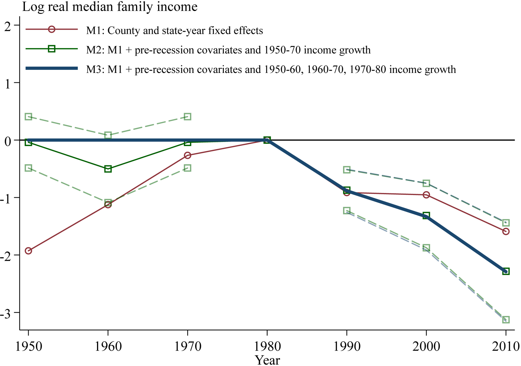
Notes: Figure plots the estimated coefficients on interactions between year and the 1979–1982 decrease in log real earnings per capita, where the coefficient for 1980 is normalized to equal zero. The dependent variable is log real median family income for 1950–1990 and log real median household income for 2000–2010. Regressions are estimated by 2SLS, using the predicted log employment change from 1979–1982 as an instrumental variable. Pre-recession covariates are year interacted with the 1950–1960, 1960–1970, and 1970–1980 log population change, and the 1960 level of log population, log population density, percent urban, percent black, percent foreign, percent with a high school degree, and percent of families with income below $3,000. Changes in log median family income are also interacted with year. For models 2 and 3, the dashed lines are pointwise 95 percent confidence intervals based on standard errors clustered by state. Sample is limited to the 2,550 counties with less than 5 percent of 1976 employment in the mining sector.
Sources: BEA Regional Economic Accounts, Census County Business Patterns, Census County Data Books, Minnesota Population Center (2011)
Figure A.3: Four-Year College Degree Attainment by Age.
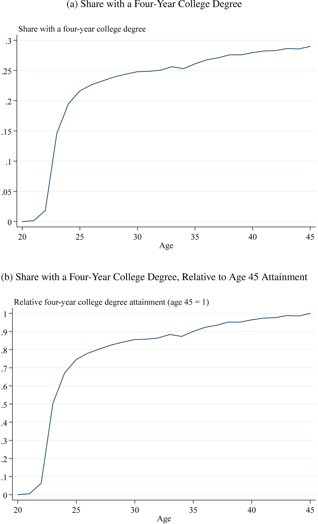
Notes: Panel A displays the share of individuals with a four-year college degree, for a constant sample of individuals born in the U.S. from 1957–1964. Panel B displays the share of attainment divided by attainment at age 45. I use custom weights from the NLS to account for the fact that these tabulations use multiple survey years.
Source: National Longitudinal Survey of Youth 1979 (1979–2010)
Figure A.4: Relationship between Severity of 1980–1982 Recession in County of Residence and County of Birth.

Notes: Figure plots OLS estimates of the interaction between the 1979–1982 decrease in log real earnings per capita in individuals’ county of birth and indicators for age. The dependent variable is the 1979–1982 decrease in log real earnings per capita in individuals’ county of residence. I estimate this relationship using confidential Census/ACS data for individuals born from 1970–2013 (county of residence observed from 2000–2013) and confidential PSID data for individuals born from 1968–1979 (county of residence observed in 1979). Both regressions include fixed effects for gender, race, and birth year-by-birth state, plus birth year interacted with the 1950–1960, 1960–1970, and 1970–1980 change in log real median family income and log population, and the 1960 level of log population, log population density, percent urban, percent black, percent foreign, percent with a high school degree, and percent of families with income below $3,000. The Census/ACS regression additionally includes fixed effects for age at time of survey by gender and age at time of survey by birth state. The dashed lines are pointwise 95 percent confidence intervals based on standard errors clustered by state. The Census/ACS sample contains 23.8 million individuals born in the continental U.S. with a unique PIK, unique birth county, and non-allocated variables. The PSID sample contains 3,684 individuals born in the continental U.S.
Sources: BEA Regional Economic Accounts, Confidential 2000–2013 Census/ACS data linked to the SSA NUMIDENT file, Confidental PSID data
Figure A.5: Comparison of Birth County Out-Migration Rates by Cohort.

Notes: Figure displays the share of individuals living outside of their birth county for different birth cohorts. In the PSID, birth county is identified based on individuals’ county of residence when first observed. I limit the PSID sample to individuals first observed before age 3.
Source: Confidental PSID data
Figure A.6: The Long-Run Effects of the 1980–1982 Recession on Four-Year College Degree Attainment, With and Without Measurement Error Adjustment.
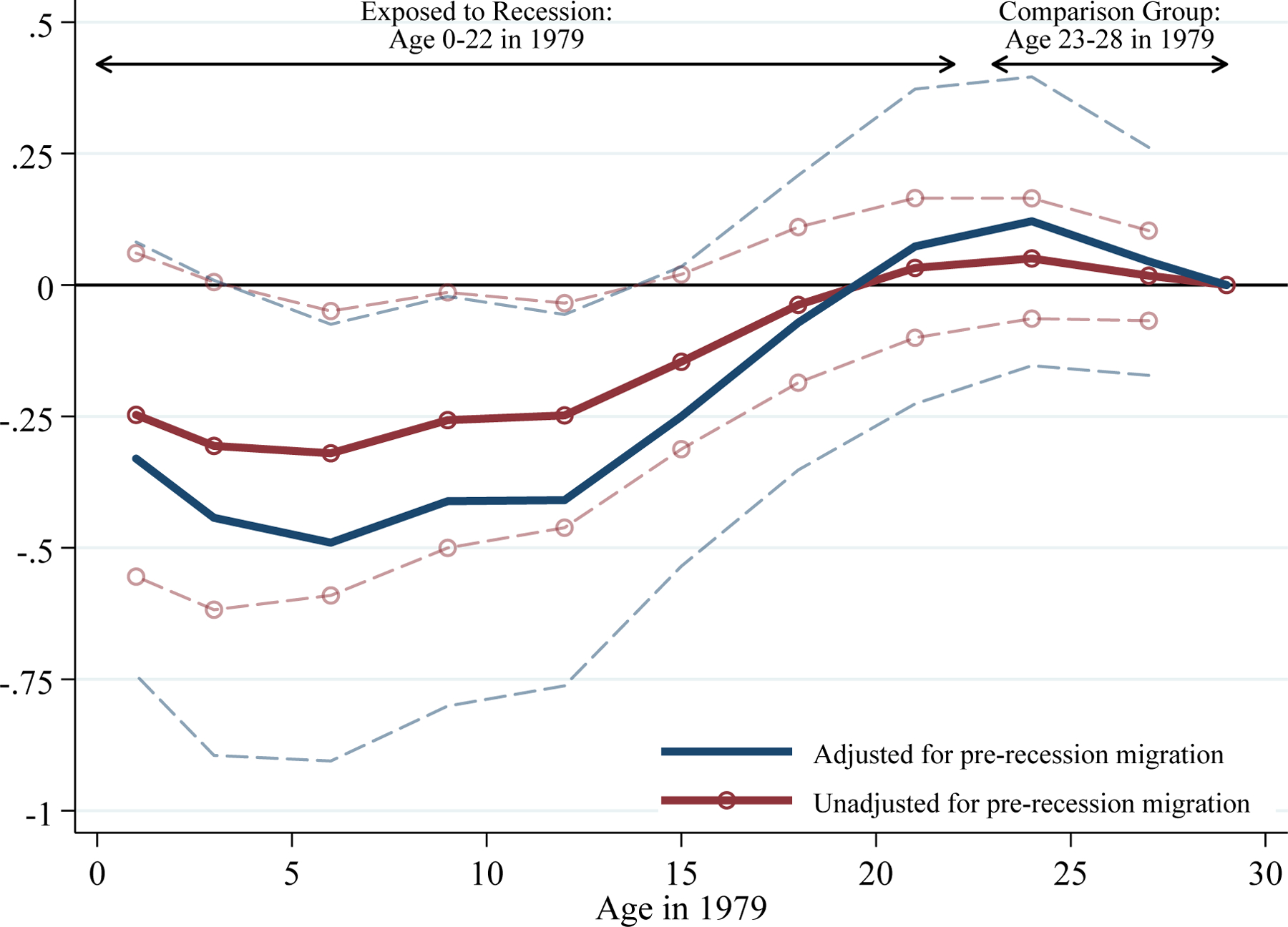
Notes: See notes to Figure 3. The dependent variable is an indicator for four-year college degree attainment. The line that adjusts for pre-recession migration divides the unadjusted estimates by the Census/ACS coefficient from Appendix Figure A.4. See Appendix D for details.
Sources: BEA Regional Economic Accounts, Census County Business Patterns, Confidential 2000–2013 Census/ACS data linked to the SSA NUMIDENT file
Figure A.7: The Long-Run Effects of the 1980–1982 Recession on Years of Schooling, With and Without Measurement Error Adjustment.

Notes: See notes to Figures 3 and A.6. The dependent variable is years of schooling.
Sources: BEA Regional Economic Accounts, Census County Business Patterns, Confidential 2000–2013 Census/ACS data linked to the SSA NUMIDENT file
Figure A.8: The Long-Run Effects of the 1980–1982 Recession on High School or GED Attainment.
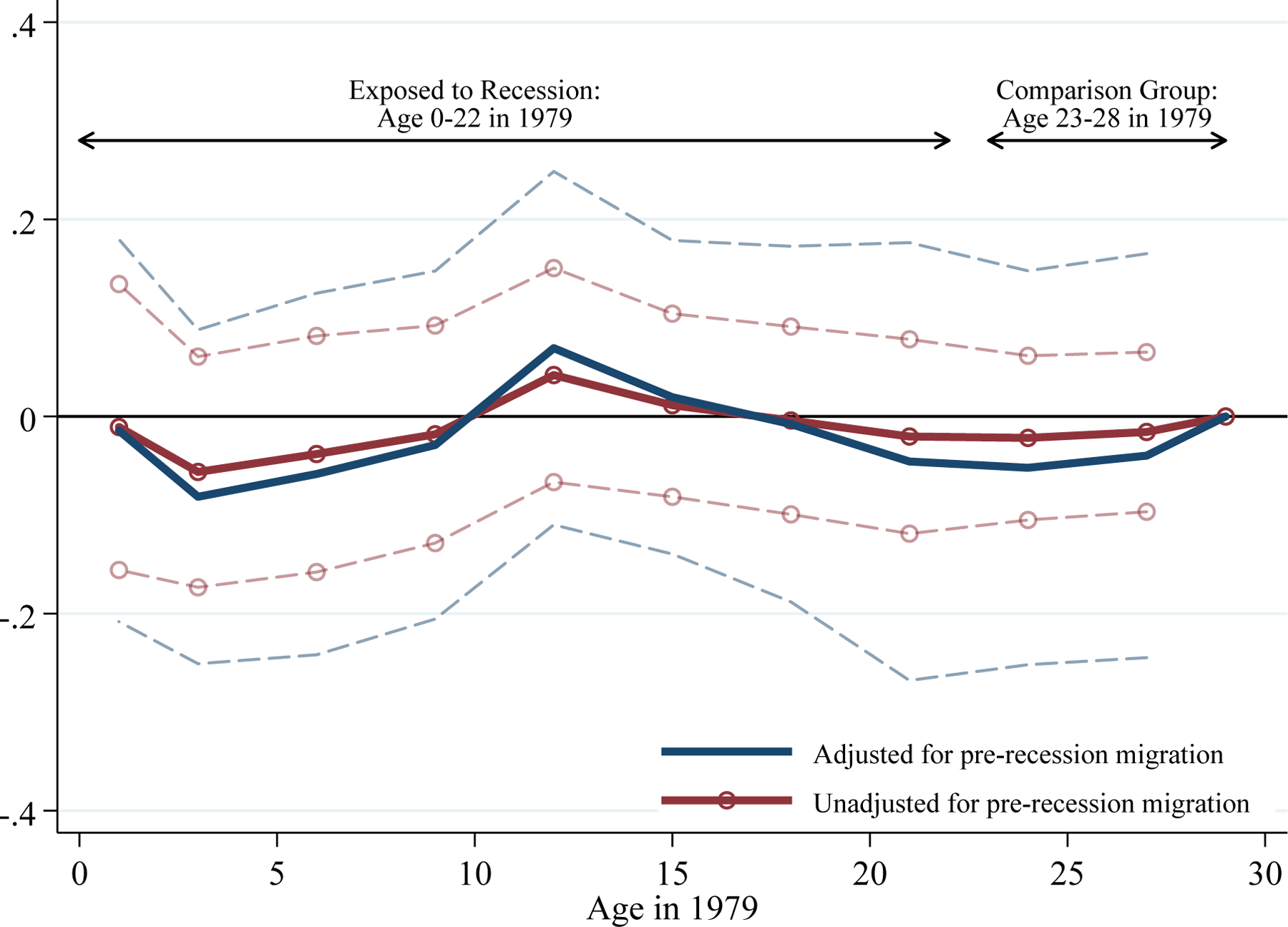
Notes: See notes to Figures 3 and A.6. The dependent variable is an indicator for high school or GED attainment. Sources: BEA Regional Economic Accounts, Census County Business Patterns, Confidential 2000–2013 Census/ACS data linked to the SSA NUMIDENT file
Figure A.9: The Long-Run Effects of the 1980–1982 Recession on Any College Attendance.

Notes: See notes to Figures 3 and A.6. The dependent variable is an indicator for any college attendance.
Sources: BEA Regional Economic Accounts, Census County Business Patterns, Confidential 2000–2013 Census/ACS data linked to the SSA NUMIDENT file
Figure A.10: The Long-Run Effects of the 1980–1982 Recession on Any College Degree Attainment.
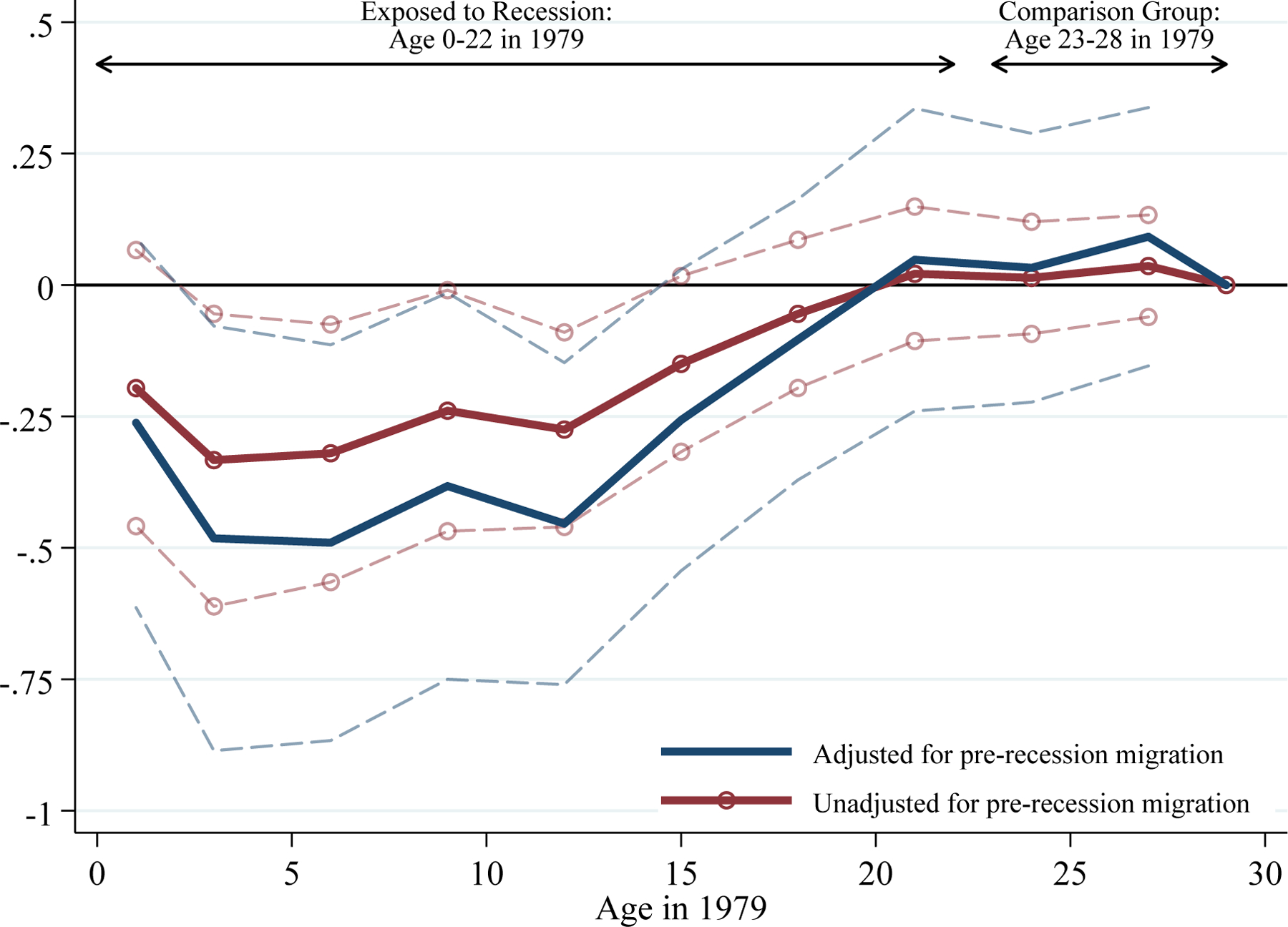
Notes: See notes to Figures 3 and A.6. The dependent variable is an indicator for any college degree attainment.
Sources: BEA Regional Economic Accounts, Census County Business Patterns, Confidential 2000–2013 Census/ACS data linked to the SSA NUMIDENT file
Figure A.11: The Long-Run Effects of the 1980–1982 Recession on Two-Year College Degree Attainment.
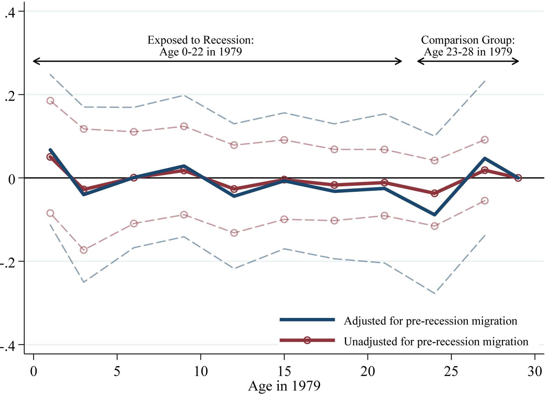
Notes: See notes to Figures 3 and A.6. The dependent variable is an indicator for two-year college degree attainment. Sources: BEA Regional Economic Accounts, Census County Business Patterns, Confidential 2000–2013 Census/ACS data linked to the SSA NUMIDENT file
Figure A.12: Summary Statistics, Income Thresholds.

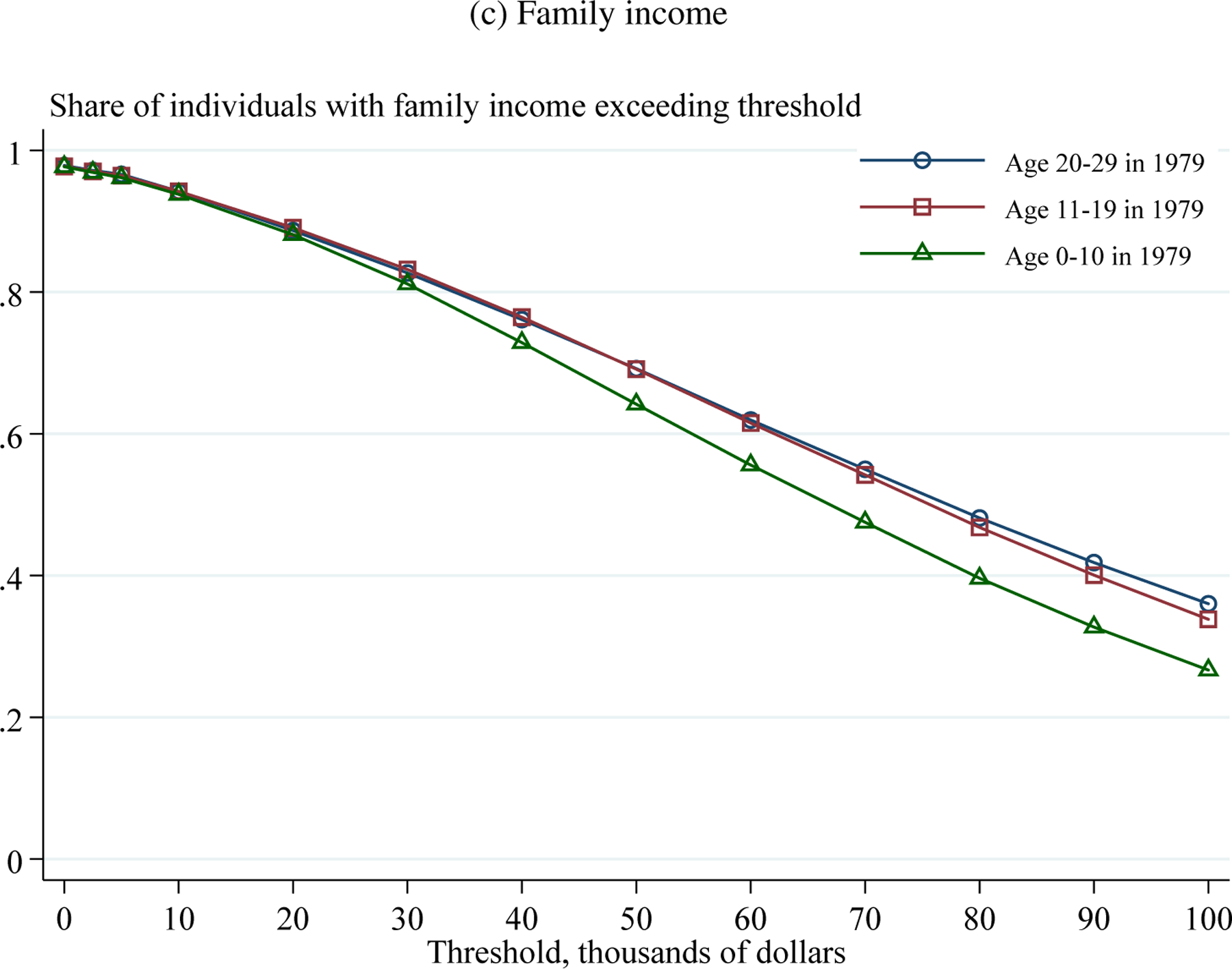
Notes: Figure reports the share of individuals with income that exceeds the indicated thresholds ($0, $2,500, $5,000, $10,000, $20,000, …, $100,000) as of 2000–2013 for the indicated birth cohort.
Sources: Publicly available 2000–2013 Census/ACS data from Ruggles et al. (2015)
Figure A.13: The Long-Run Effects of the 1980–1982 Recession on Log Personal Income.

Notes: See notes to Figure 3 and Table 3. The dependent variable is log personal income.
Sources: BEA Regional Economic Accounts, Census County Business Patterns, Confidential 2000–2013 Census/ACS data linked to the SSA NUMIDENT file
Figure A.14: The Long-Run Effects of the 1980–1982 Recession on Log Earned Income.

Notes: See notes to Figure 3 and Table 3. The dependent variable is log earned income.
Sources: BEA Regional Economic Accounts, Census County Business Patterns, Confidential 2000–2013 Census/ACS data linked to the SSA NUMIDENT file
Figure A.15: The Long-Run Effects of the 1980–1982 Recession on Log Family Income.
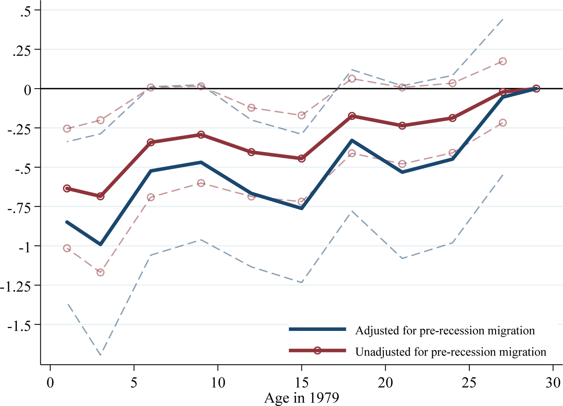
Notes: See notes to Figure 3 and Table 3. The dependent variable is log family income.
Sources: BEA Regional Economic Accounts, Census County Business Patterns, Confidential 2000–2013 Census/ACS data linked to the SSA NUMIDENT file
Figure A.16: The Long-Run Effects of the 1980–1982 Recession on Log Hourly Wage.

Notes: See notes to Figure 3 and Table 3. The dependent variable is log hourly wage.
Sources: BEA Regional Economic Accounts, Census County Business Patterns, Confidential 2000–2013 Census/ACS data linked to the SSA NUMIDENT file
Figure A.17: The Long-Run Effects of the 1980–1982 Recession on Poverty.

Notes: See notes to Figure 3 and Table 3. The dependent variable is an indicator for being in poverty.
Sources: BEA Regional Economic Accounts, Census County Business Patterns, Confidential 2000–2013 Census/ACS data linked to the SSA NUMIDENT file
Figure A.18: Infant Mortality Before the 1980–1982 Recession.
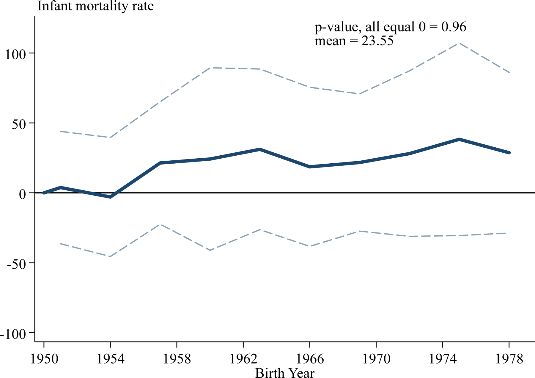
Notes: Figure plots the estimated coefficients on interactions between birth year and the 1979–1982 decrease in log real earnings per capita, where the coefficient for 1950 is normalized to equal zero. The dependent variable is the infant mortality rate (deaths per 1,000 births). The regression is estimated by 2SLS, using the predicted log employment change from 1979–1982 as an IV. The regression includes the share of births to nonwhite mothers and fixed effects for county and state-by-year, plus year interacted with the 1950–1960, 1960–1970, and 1970–1980 change in log real median family income and log population, and the 1960 level of log population, log population density, percent urban, percent black, percent foreign, percent with a high school degree, and percent of families with income below $3,000. The dashed lines are pointwise 95 percent confidence intervals based on standard errors clustered at the birth state level. Sample is limited to the 2,550 counties with less than 5 percent of 1976 employment in the mining sector.
Sources: Bailey et al. (2018), BEA Regional Economic Accounts, Census County Business Patterns, Census County Data Books, Minnesota Population Center (2011)
Figure A.19: Birth Rates and the 1980–1982 Recession.
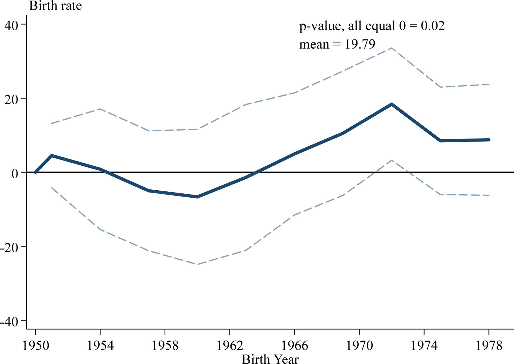
Notes: Figure plots the estimated coefficients on interactions between birth year and the 1979–1982 decrease in log real earnings per capita, where the coefficient for 1950 is normalized to equal zero. The dependent variable is the birth rate (births per 1,000 people). The regression is estimated by 2SLS, using the predicted log employment change from 1979–1982 as an IV. The regression includes the share of births to nonwhite mothers and fixed effects for county and state-by-year, plus year interacted with the 1950–1960, 1960–1970, and 1970–1980 change in log real median family income and log population, and the 1960 level of log population, log population density, percent urban, percent black, percent foreign, percent with a high school degree, and percent of families with income below $3,000. The dashed lines are pointwise 95 percent confidence intervals based on standard errors clustered at the birth state level. Sample is limited to the 2,550 counties with less than 5 percent of 1976 employment in the mining sector.
Sources: Bailey et al. (2018), BEA Regional Economic Accounts, Census County Business Patterns, Census County Data Books, Minnesota Population Center (2011)
Figure A.20: Distribution of Inverse Hyperbolic Sine of Income Measures, 2000–2013.


Notes: Figure displays histograms of inverse hyperbolic sine of indicated income measures for individuals age 25–64 observed in the 2000 Census and 2001–2013 ACS.
Sources: Public Use Census/ACS Data
Footnotes
For example, negative effects from a decline in earnings could be offset by positive long-run effects from a reduction in pollution (Chay and Greenstone, 2003; Isen, Rossin-Slater and Walker, 2017; Voorheis, 2017). My sample only includes individuals born before the recession, so effects on in-utero development are not operative.
Work examining the short-run effects of labor market opportunities and parental job loss on children includes Rege, Telle and Votruba (2011); Stevens and Schaller (2011); Ananat et al. (2013); Schaller and Stevens (2015); Schaller and Zerpa (2019).
Most closely related is recent work by Cutler, Huang and Lleras-Muney (2016) and Rao (2016), who examine the long-run effects of detrended GDP and unemployment rate fluctuations that occur during childhood. These fluctuations equal zero on average, and below-trend fluctuations tend to be followed by above-trend fluctuations, so their estimates do not speak directly to the effects of a recession. Studies on the long-run effects of parental job displacement (Page, Stevens and Lindo, 2007; Bratberg, Nilsen and Vaage, 2008; Oreopoulos, Page and Stevens, 2008; Coelli, 2011; Hilger, 2016) also are related, but do not directly assess the effects of recessions, which might operate through additional channels besides parental job loss, such as schools, neighborhoods, and peers. Similarly, studies on the effects of parental income (e.g., Løken, 2010; Løken, Mogstad and Wiswall, 2012) do not directly assess the effects of recessions.
Recent studies on the effect of entry labor market conditions on workers include Kahn (2010); Hershbein (2012); Oreopoulos, von Wachter and Heisz (2012); Altonji, Kahn and Speer (2016); Speer (2016).
This paper does not analyze the desirability of social insurance or economic stabilization policies, but such an analysis depends in part on the long-run effects documented in this paper.
The NBER recession dates are January to July 1980 and July 1981 to November 1982. I treat these as a single episode, using 1979 as the pre-recession year.
Table 1 is based on annual Census County Business Patterns data. While total employment in these data grew by 467,000 jobs during this period, monthly data from the Bureau of Labor Statistics Current Employment Statistics show large employment decreases in the first half of 1980 and from 1981 to 1982.
The unweighted average decrease in log earnings per capita is 6.4 percent, and the standard deviation is 10.6 percent. Using 1979 population weights, the average decrease is 4.8 percent, and the standard deviation is 6.5 percent.
Greenstone and Looney (2010) document a similar finding for the 1980–1982 recession.
Jaimovich and Siu (2015) and Hershbein and Kahn (2018) discuss factors that could lead to persistent declines in local economic activity, although they focus on more recent recessions.
An income effect also could arise from a decline in house prices and parental wealth. Some studies find that children’s long-run outcomes are sensitive to changes in family resources (Aizer et al., 2016; Hoynes, Schanzenbach and Almond, 2016), while others do not (Jacob, Kapustin and Ludwig, 2015; Bleakley and Ferrie, 2016). Bulman et al. (2016) find that college attendance is sensitive only to very large increases in income.
Aguiar, Hurst and Karabarbounis (2013) find that parents spent more time with children during the Great Recession, and Del Boca, Flinn and Wiswall (2014) find that parental time produces cognitive skills in children. Additional time might have limited benefits, or even be harmful, if the recession increases parental stress (McLoyd et al., 1994; Leininger and Kalil, 2014; Brand, 2015; Akee et al., 2018).
Existing work documents long-run effects of both disruptive peers (Carrell, Hoekstra and Kuka, 2018) and neighborhoods (Chetty, Hendren and Katz, 2016; Chetty and Hendren, 2018a; Chyn, 2018).
Some empirical work finds an important role for opportunity cost in educational attainment (Black, McKinnish and Sanders, 2005; Atkin, 2016; Charles, Hurst and Notowidigdo, 2018; Cascio and Narayan, 2019). Bound and Holzer (2000) and Hoynes, Miller and Schaller (2012) show that the 1980–1982 recession especially reduced the wages and employment of less educated workers.
Several studies conclude that short-term credit constraints are relatively unimportant for college attendance or graduation (Cameron and Heckman, 2001; Cameron and Taber, 2004; Stinebrickner and Stinebrickner, 2008; Bulman et al., 2016), but some evidence from college decisions made in the early 2000s suggests a larger role for credit constraints (Belley and Lochner, 2007; Bailey and Dynarski, 2011; Lovenheim, 2011). Charles, Hurst and Notowidigdo (2018) find that the early 2000s housing boom decreased college enrollment, consistent with opportunity cost being more important than parental resources in their setting.
These samples balance the goals of using as much information as possible, given non-trivial allocation rates for labor market outcomes, and limiting the number of samples to ensure that no confidential information is disclosed. In publicly available 2000–2013 Census/ACS data, for people born in the U.S. from 1950–1979 who are age 25–64 at the time of the survey, 8.1 percent of individuals have allocated age, gender, race, or state of birth. Among individuals with no allocations in these variables, 1.8 percent are in group quarters. A further 1.1 percent of individuals have allocated years of education, and 21.3 percent have allocated education or labor market variables (any of the seven individual income variables, total family income, weeks worked, hours worked, marital status, and labor force status).
The Census Bureau assigns PIKs to individuals in the Census and ACS using information on respondents’ name, address, date of birth, and gender. Sometimes a PIK is assigned to more than one respondent in a survey year. While technically possible (e.g., if an individual receives a survey at multiple residences), this outcome likely reflects an error in PIK assignment. An individual may be assigned to multiple birth counties if the 12-character string from the NUMIDENT does not identify a single county. For example, there are two towns named Arcadia in North Carolina, and a respondent who writes “Arcadia” could be matched to two counties. Appendix A describes the algorithm that identifies county of birth using the 12-character place of birth string in the NUMIDENT.
Recessions could affect higher education access and transfer program expenditures, but there are many other determinants of these programs. Given the conceptual and practical challenges of controlling for changes due to factors besides the recession, I prefer to include age in 1979-by-birth state fixed effects.
I use the predicted log employment change because earnings data are not available at a sufficiently detailed industry level. I exclude the contribution from a county’s own state to remove a mechanical relationship between the actual and predicted change in economic activity. Using other states in the same region, as opposed to all other states, allows industry-level employment changes to differ by region. I construct using Census County Business Patterns (CBP) data. CBP data frequently suppress employment for county-by-industry cells to protect respondent confidentiality, but never suppress the number of establishments within establishment size categories. I impute CBP employment using the number of establishments and nationwide information on employment by establishment size, as described in Appendix C.
For individuals born from 1957–1964, about 75 percent of four-year college degree attainment is completed by age 25 and 85 percent is completed by age 29 (Appendix Figure A.3).
The potential impacts of the recession on older individuals also means that there is no falsification test for income.
The bins are for 1979 ages 0–1, 2–4, 5–7, 8–10, 11–13, 14–16, 17–19, 20–22, 23–25, and 26–28.
Appendix Figures A.8–A.11 present results for other measures of educational attainment.
Appendix E discusses the first stage, reduced-form, and OLS estimates. First stage F-statistics range from 43 to
Census/ACS data measure the highest degree completed, so an individual with a two- and four-year degree is recorded as having a four-year degree.
Appendix Figure A.12 reports the share of individuals with income exceeding each threshold.
Earned income is wage and salary plus business and farm income. Personal income is the sum of earned, welfare, Social Security, Supplementary Security, investment, retirement, and other income. To limit the influence of potential outliers in the self-reported income data, for each income category I replace values above the 99.5th percentile in each survey year by state of residence cell with the average among those above the 99.5th percentile. I construct earned and personal income as the sum of the non-allocated, top-code-adjusted components.
In constructing family income and poverty rates, I separate extended families living in the same household (see Hoynes, Page and Stevens, 2006). I create fa mily interrelationship variables in the confidential Census/ACS data that mirror those constructed by Ruggles et al. (2015) in IPUMS data.
A 1 SD increase in the severity of the recession amounts to a 10.6 percent decrease in earnings per capita from 1979–1982, which leads to a 4.2 percent decrease in family income. Chetty and Hendren (2018b) find that spending 20 years in a 1 SD worse county leads to a 10.4 percent decrease in earnings for children of parents at the 25th percentile of the income distribution, and a 6.4 percent decrease in earnings for children of parents at the 75th percentile. Taking the average of these yields an 8.4 percent decrease in earnings.
Appendix Figures A.13–A.17 present estimates for income, wages, and poverty using finer age categories.
Because the recession reduces college degree attainment, the effect of the recession on early career income is likely less negative than the effect on lifetime income. The effect on late career income (e.g., for individuals age 29 in 1979) could be more negative than the effect on lifetime income, in part because early career income is earned before the recession. Both considerations lead to an upwards bias in the difference-in-differences estimates, with this bias being more severe for younger individuals. Haider and Solon (2006) find substantial life-cycle bias up to age 30. Because the 2000 Census has more observations than the 2001–2013 ACS samples, my estimates place higher weight on earlier ages, which suggests that life-cycle bias could be quantitatively important.
I use 2000–2013 Census/ACS data to regress log income and log wages on indicators for high school/GED attainment, college attendance, two-year degree attainment, and four-year degree attainment, plus indicators for gender-by-age, race, and year.
Appendix Table A.10 shows small within-state correlations between the change in log earnings per capita from 1979–1982 and during other recessions, and small within-state correlations between the predicted log employment change from 1979–1982 and the log earnings per capita change during other recessions. There is little correlation between the log earnings per capita change or predicted log employment change from 1979–1982 and Japanese import competition as measured by Batistich and Bond (2019) or Chinese import competition as measured by Autor, Dorn and Hanson (2013).
These papers find that job displacement leads to long-run reductions in family income of around 10 percent. They do not estimate the effect of parental job displacement on college degree attainment.
Previous studies suggest that if job loss generated all of the county-level decrease in earnings per capita from 1979–1982 and the recession only affected children whose parents lost a job, then a 10 percent decrease in earnings per capita would decrease earned income by 0–9 percent (Page, Stevens and Lindo, 2007; Bratberg, Nilsen and Vaage, 2008; Oreopoulos, Page and Stevens, 2008; Hilger, 2016). For individuals age 11–19 in 1979, Table 3 implies that a 10 percent decrease in earnings per capita leads to a 3 percent decrease in earned income.
As shown in Appendix Figures A.8 and A.9, I do not find significant long-run effects on high school degree attainment or college attendance for older cohorts. Previous research on the relationship between economic conditions and high school and college enrollment yields mixed results. Betts and McFarland (1995) and Clark (2011) find significant positive relationships between enrollment and unemployment rates. Conclusions are similar from studies of specific shocks by Black, McKinnish and Sanders (2005), Charles, Hurst and Notowidigdo (2018), and Cascio and Narayan (2019). Card and Lemieux (2001), Christian (2007), and Barr and Turner (2013) generally do not find statistically significant relationships, although Barr and Turner (2013) find a stronger positive relationship between unemployment and enrollment around the Great Recession.
Appendix Figures A.14 and A.16 imply that a 10 percent decrease in earnings per capita leads to a statistically insignificant 3.6 percent decrease in earned income and hourly wages for individuals age 22 in 1979. This is consistent with some of the estimates in Kahn (2010), and the estimates in Oreopoulos, von Wachter and Heisz (2012) and Altonji, Kahn and Speer (2016), which imply that college graduates’ earnings and wages recover after 10 or 15 years. Prior work does not find persistent effects of labor market conditions at entry on workers with less than a college degree (Hershbein, 2012; Speer, 2016).
In constructing the dependent variable, I focus on transfers over which states have some statutory or administrative control: retirement and disability insurance (excluding Social Security), Medicare, public assistance medical care benefits (primarily Medicaid), income maintenance benefits (including Food Stamps and AFDC), unemployment insurance compensation, and education and training assistance. Appendix Table A.18 characterizes the generosity and progressivity of state transfer systems.
Appropriations in 1970 have the advantage of being determined before the recession, but they imperfectly measure higher education funding when individuals made their schooling decision. Post-recession appropriations are difficult to interpret because they might have been affected by the recession. The same is true of overall transfers and transfer progressivity.
Card and Payne (2002) use a similar approach to characterize state-level school aid systems.
This indicates that the evolution of earnings per capita from 1982–1992 is not a confounding omitted variable in my main specification, consistent with a relatively small correlation between the severity of the recession and the post-recession evolution of economic activity (e.g., see Figure 2).
In 2015, there were 69 million individuals with a four-year college degree (Ryan and Bauman, 2016) and 43 million individuals living in poverty (Proctor, Semega and Kollar, 2016). In 2014 dollars, U.S. GDP was $9.0 trillion in 1979 and $18.2 trillion in 2015.
These simple calculations do not capture cohort-wide effects or general equilibrium adjustments. The resulting bias from not capturing cohort-wide effects is unclear, as these effects could be positive or negative, while general equilibrium adjustments suggest that these calculations might overstate the aggregate effects. For example, increasing the college degree attainment of individuals born in one county might decrease the attainment of individuals born in other counties due to less than perfect elasticity of supply of college education (Bound and Turner, 2007). These calculations could understate the true aggregate effects because they only include individuals born from 1960–1979, and the recession could have negative effects on earnings of people born before 1960 and on education and earnings of people born after 1979.
The figure plots the percent difference in earnings per capita between counties with a more versus less severe recession, normalized to equal zero at the onset of the recession. The counties with a more versus less severe recession are defined separately for each recession.
45 We restrict attention to geographic features that are plausibly populated (those with a Populated Place, Census, or Civil feature class) or have a federal location code.
For example, there are three different Populated Places in North Carolina beginning with “Bells Crossroads” located in different counties. Repeated place names pose less of a problem if the place name has less than 12 characters. For example, there are two places named Arcadia in North Carolina: one in Davidson County and the other in Forsyth County. These can be distinguished if “Arcadia Davi” or “Arcadia Fors” appear in the NUMIDENT.
For example, a person born in North Carolina who writes “Arcadia Fors” or “Arcadia Davi” is matched to the correct Arcadia (in Forsyth or Davidson county) in the exact matching step. However, if an individual writes “Arcadia,” we do not know in which Arcadia they were born. If at least 75 percent of the exact Arcadia matches are attributed to one county, then we match “Arcadia” to that county.
In the probabilistic matching step, we only match NUMIDENT strings to GNIS places that have census codes to control the number of false positive matches. We first use the Stata command reclink2 (Wasi and Flaaen, 2015), with the tolerance set to 0.1, to obtain a set of potential matches for each NUMIDENT string. We then use the Stata command jarowinkler (Feigenbaum, 2015) to select the best match as the one with the highest Jaro-Winkler score among the potential matches. If no potential match has a Jaro-Winkler score of at least 0.8, then the string remains unmatched. If multiple places have the same Jaro-Winkler score, then this step matches to each place.
I use median family income because it is available at the county-level from decennial Censuses for 1950–2000 (and the ACS for 2010) and is an important measure of local economic conditions. County-level Census data do not consistently report other quantiles of the family income distribution from 1950–2010.
When including the 526 counties with at least 5 percent of 1976 employment in mining, log median family income evolves similarly from 1950–1970, but declines by less after 1980. Because relatively few people live in high mining counties, my estimates of long-run effects on children more closely reflect the persistence seen in Figure A.2, which excludes high mining counties.
These orthogonality conditions imply that is orthogonal to , and hence that εi,a,c,t is orthogonal to . Alternatively, I could assume that εi,a,c,t is orthogonal to , which would imply that is orthogonal to , and hence that is orthogonal to .
An alternative approach is to define as the average change in log earnings per capita for individuals who were age a in 1979 and born in county c, and note that , where pa,c,k is the share of individuals age a in 1979 who were born in county c and resided in county k in 1979. Estimates of pa,c,k would allow me to construct directly. I do not pursue this approach because the measurement error correction for each cohort depends on nearly 9.5 million parameters (≈ 30762), and adequate data on county-to-county migration flows are not available.
Data on infant birth weight are available starting in 1968, and data on maternal education are available starting in 1969. I focus on 1970-forward because the 1969 data handle births to nonresident aliens differently than the 1970-forward data.
For results on maternal education, I restrict the sample to states that reported education throughout the 1970–1979 period. This results in the exclusion of 13 states (Alabama, Arkansas, California, Connecticut, Delaware, the District of Columbia, Georgia, Idaho, Maryland, New Mexico, Pennsylvania, Texas, and Washington).
Mean real earnings per capita in 1979 is $21,822, so a 10 percent decrease in earnings per capita at the mean amounts to $2,182. The estimates using the decrease in earnings per capita in Appendix Table A.14 imply that a $2,182 decrease in earnings per capita leads to a 4.9 percentage point (=0.223 × 0.2182) decrease in four-year degree attainment for 0–10 year olds and a 3.0 percentage point decrease for 11–19 year olds. These estimates are similar to those which use the change in log real earnings per capita, which imply a 4.7 and 2.9 percentage point decrease.
In a very small number of instances, a county reports 0 expenditures or revenues for the outcomes I examine. To maintain a constant sample, I use the inverse hyperbolic sine, , instead of ln(y) throughout (Burbridge, Magee and Robb, 1988). The log and inverse hyperbolic sine yield very similar coefficients in linear regression models when y is sufficiently large.
I downloaded these data from the NBER website, with thanks to Michael Greenstone for making them available. I exclude the five New York City counties from the analysis because they are combined into a single geographic unit.
I exclude liquor stores, utilities (water supply, electric power, gas supply, and mass transit), and insurance trusts to focus on government activities most likely to affect children, but results are similar when including these categories. I exclude intergovernmental expenditures to avoid double counting, which could arise when a county government gives money to a school district, which then spends the money on teachers’ salaries. The grouping of expenditures and revenues in Appendix Tables A.16 and A.17 is similar to that used by Bartik et al. (2019).
Education expenditure purposes include elementary and secondary education, higher education, and libraries. Public safety expenditure purposes include police, correctional facilities, fire, judicial and legal, and protective inspection and regulation. Welfare and health expenditure purposes include welfare, health and hospital, transit subsidies, and housing and community development. Infrastructure expenditure purposes include airport, total highway, parking, sewerage, solid wage management, and water transport and terminals. Examples of other expenditure purposes are financial administration, central staffing, and parks and recreation.
As expected given balanced budget requirements, the change in expenditures in Appendix Table A.16 approximately mirror the change in revenues in Appendix Table A.17.
References
- Aguiar Mark, Hurst Erik, and Karabarbounis Loukas. 2013. “Time Use during the Great Recession.” American Economic Review, 103(5): 1664–1696. [Google Scholar]
- Aizer Anna, Eli Shari, Ferrie Joseph, and Lleras-Muney Adriana. 2016. “The Long Term Impact of Cash Transfers to Poor Families.” American Economic Review, 106(4): 935–971. [DOI] [PMC free article] [PubMed] [Google Scholar]
- Akee Randall, Copeland William, Costello E. Jane, and Simeonova Emilia. 2018. “How Does Household Income Affect Child Personality Traits and Behaviors?” American Economic Review, 108(3): 775–827. [DOI] [PMC free article] [PubMed] [Google Scholar]
- Almond Douglas, and Currie Janet. 2011. “Human Capital Development before Age Five.” In Handbook of Labor Economics. Vol. 4B, ed. Card David and Ashenfelter Orley, 1315–1486. Elsevier. [Google Scholar]
- Almond Douglas, Currie Janet, and Duque Valentina. 2018. “Childhood Circumstances and Adult Outcomes: Act II.” Journal of Economic Literature, 56(4): 1360–1446. [Google Scholar]
- Altonji Joseph G., Kahn Lisa B., and Speer Jamin D.. 2016. “Cashier or Consultant? Entry Labor Market Conditions, Field of Study, and Career Success.” Journal of Labor Economics, 34(1): S361–S401. [Google Scholar]
- Ananat Elizabeth Oltmans, Anna Gassman-Pines, Francis Dania V. and Gibson-Davis Christina M.. 2013. “Children Left Behind: The Effects of Statewide Job Loss on Student Achievement.” NBER Working Paper 17104. [Google Scholar]
- Atkin David. 2016. “Endogenous Skill Acquisition and Export Manufacturing in Mexico.” American Economic Review, 106(8): 2046–2085. [Google Scholar]
- Autor David, Figlio David, Karbownik Krzysztof, Roth Jeffrey, and Wasserman Melanie. 2019. “Family Disadvantage and the Gender Gap in Behavioral and Educational Outcomes.” American Economic Journal: Applied Economics, 11(3): 338–381. [Google Scholar]
- Autor David H., Dorn David, and Hanson Gordon H.. 2013. “The China Syndrome: Local Labor Market Effects of Import Competition in the United States.” American Economic Review, 103(6): 2121–2168. [Google Scholar]
- Bailey Martha J., and Dynarski Susan M.. 2011. “Inequality in Postsecondary Education.” In An Economic Perspective on the Problems of Disadvantaged Youth. ed. Duncan Greg J. and Murnane Richard J., 117–131. New York: Russell Sage Foundation. [Google Scholar]
- Bailey Martha J., Clay Karen, Fishback Price, Haines Michael R., Kantor Shawn, Severnini Edson, and Wentz Anna. 2018. “U.S. County-Level Natality and Mortality Data, 1915–2007. Ann Arbor, MI: ICPSR; [distributor].” [Google Scholar]
- Barnett Barry J. 2000. “The U.S. Farm Financial Crisis of the 1980s.” Agricultural History, 74(2): 366–380. [Google Scholar]
- Barr Andrew, and Turner Sarah E.. 2013. “Expanding Enrollments and Contracting State Budgets: The Effect of the Great Recession on Higher Education.” The Annals of the American Academy of Political and Social Science, 650: 168–193. [Google Scholar]
- Bartik Alexander W., Currie Janet, Greenstone Michael, and Knittel Christopher R.. 2019. “The Local Economic and Welfare Consequences of Hydraulic Fracturing.” American Economic Journal: Applied Economics, 11(4): 105–55. [Google Scholar]
- Bartik Timothy J. 1991. Who Benefits from State and Local Economic Development Policies? Kalamazoo, Michigan: W.E. Upjohn Institute for Employment Research. [Google Scholar]
- Bartik Timothy J. 1993. “Who Benefits from Local Job Growth: Migrants or the Original Residents?” Regional Studies, 27(4): 297–311. [DOI] [PubMed] [Google Scholar]
- Batistich Mary Kate, and Bond Timothy N.. 2019. “Stalled Racial Progress and Japanese Trades in the 1970s and 1980s.” [Google Scholar]
- Becker Gary S. 1962. “Investment in Human Capital: A Theoretical Analysis.” Journal of Politi cal Economy, 70(5): 9–49. [Google Scholar]
- Belley Philippe, and Lochner Lance. 2007. “The Changing Role of Family Income and Ability in Determining Educational Achievement.” Journal of Human Capital, 1(1): 37–89. [Google Scholar]
- Ben-Porath Yoram. 1967. “The Production of Human Capital and the Life Cycle of Earnings.” Journal of Political Economy, 75(4): 352–365. [Google Scholar]
- Betts Julian R., and McFarland Laurel L.. 1995. “Safe Port in a Storm: The Impact of Labor Market Conditions on Community College Enrollments.” Journal of Human Resources, 30(4): 741–765. [Google Scholar]
- Black Dan A., McKinnish Terra G., and Sanders Seth G.. 2005. “Tight Labor Markets and the Demand for Education: Evidence from the Coal Boom and Bust.” Industrial and Labor Relations Review, 59(1): 3–16. [Google Scholar]
- Blanchard Olivier Jean, and Katz Lawrence F.. 1992. “Regional Evolutions.” Brookings Papers on Economic Activity. [Google Scholar]
- Bleakley Hoyt, and Ferrie Joseph. 2016. “Shocking Behavior: Random Wealth in Ante-bellum Georgia and Human Capital Across Generations.” Quarterly Journal of Economics, 131(3): 1455–1495. [DOI] [PMC free article] [PubMed] [Google Scholar]
- Bound John, and Holzer Harry J.. 2000. “Demand Shifts, Population Adjustments, and Labor Market Outcomes during the 1980s.” Journal of Labor Economics, 18(1): 20–54. [Google Scholar]
- Bound John, and Turner Sarah. 2007. “Cohort Crowding: How Resources Affect Collegiate Attainment.” Journal of Public Economics, 91(5–6): 877–899. [Google Scholar]
- Bound John, Lovenheim Michael F., and Turner Sarah. 2010. “Why Have College Completion Rates Declined? An Analysis of Changing Student Preparation and Collegiate Resources.” American Economic Journal: Applied Economics, 2(3): 129–57. [DOI] [PMC free article] [PubMed] [Google Scholar]
- Brand Jennie E. 2015. “The Far-Reaching Impact of Job Loss and Unemployment.” Annual Review of Economics, 41: 359–375. [DOI] [PMC free article] [PubMed] [Google Scholar]
- Bratberg Espen, Nilsen Øivind Anti, and Vaage Kjell. 2008. “Job Losses and Child Outcomes.” Labour Economics, 15(1): 591–603. [Google Scholar]
- Bulman George, Fairlie Robert, Goodman Sarena, and Isen Adam. 2016. “Parental Resources and College Attendance: Evidence from Lottery Wins.” NBER Working Paper 22679. [Google Scholar]
- Burbridge John B., Magee Lonnie, and Robb A. Leslie. 1988. “Alternative Transformations to Handle Extreme Values of the Dependent Variable.” Journal of the American Statistical Association, 83(401): 123–127. [Google Scholar]
- Caballero Ricardo J., and Hammour Mohamad L.. 1994. “The Cleansing Effect of Recessions.” American Economic Review, 84(5): 1350–1368. [Google Scholar]
- Cameron Stephen V., and Taber Christopher. 2004. “Estimation of Educational Borrowing Constraints Using Returns to Schooling.” Journal of Political Economy, 112(1): 132–182. [Google Scholar]
- Cameron Stephen V., and Heckman James J.. 2001. “The Dynamics of Educational Attainment for Black, Hispanic, and White Males.” Journal of Political Economy, 109(3): 455–499. [Google Scholar]
- Card David, and Payne A. Abigail. 2002. “School Finance Reform, The Distribution Of School Spending, And The Distribution Of Student Test Scores.” Journal of Public Economics, 83(1): 49–82. [Google Scholar]
- Card David, and Lemieux Thomas. 2001. “Dropout and Enrollment Trends in the Postwar Period: What Went Wrong in the 1970s?” Risky Behavior among Youths: An Economic Analysis, 439–482. University of Chicago Press. [Google Scholar]
- Carrell Scott E., Hoekstra Mark, and Kuka Elira. 2018. “The Long-Run Effects of Disruptive Peers.” American Economic Review, 108(11): 3377–3415. [Google Scholar]
- Cascio Elizabeth U., and Narayan Ayushi. 2019. “Who Needs a Fracking Education? The Educational Response to Low-Skill Biased Technological Change.” [Google Scholar]
- Chambers MM 1972–1973. “Appropriations of State Tax Funds for Operating Expenses of Higher Education.” Accessed via https://education.illinoisstate.edu/grapevine/historical/. [Google Scholar]
- Charles Kerwin Kofi, Hurst Erik, and Notowidigdo Matthew J.. 2018. “Housing Booms and Busts, Labor Market Opportunities, and College Attendance.” American Economic Review, 108(10): 2947–94. [Google Scholar]
- Chay Kenneth Y., and Greenstone Michael. 2003. “The Impact of Air Pollution on Infant Mortality: Evidence from Geographic Variation in Pollution Shocks Induced by a Recession.” Quarterly Journal of Economics, 118(3): 1121–1167. [Google Scholar]
- Chetty Raj, and Hendren Nathaniel. 2018a. “The Impacts of Neighborhoods on Intergenerational Mobility I: Childhood Exposure Effects.” The Quarterly Journal of Economics, 133(3): 1107–1162. [Google Scholar]
- Chetty Raj, and Hendren Nathaniel. 2018b. “The Impacts of Neighborhoods on Intergenerational Mobility II: County-Level Estimates.” The Quarterly Journal of Economics, 133(3): 1163–1228. [Google Scholar]
- Chetty Raj, Hendren Nathaniel, and Katz Lawrence F.. 2016. “The Effects of Exposure to Better Neighborhoods on Children: New Evidence from the Moving to Opportunity Experiment.” American Economic Review, 106(4): 855–902. [DOI] [PubMed] [Google Scholar]
- Christian Michael S. 2007. “Liquidity Constraints and the Cyclicality of College Enrollment in the United States.” Oxford Economic Papers, 59(1): 141–169. [Google Scholar]
- Chyn Eric. 2018. “Moved to Opportunity: The Long-Run Effects of Public Housing Demolition on Children.” American Economic Review, 108(10): 3028–56. [DOI] [PMC free article] [PubMed] [Google Scholar]
- Clark Damon. 2011. “Do Recessions Keep Students in School? The Impact of Youth Unemployment on Enrolment in Post-compulsory Education in England.” Economica, 78(311): 523–545. [Google Scholar]
- Coelli Michael B. 2011. “Parental Job Loss and the Education Enrollment of Youth.” Labour Economics, 18(1): 25–35. [Google Scholar]
- Cutler David M., Huang Wei, and Lleras-Muney Adriana. 2016. “Economic Conditions and Mortality: Evidence from 200 Years of Data.” NBER Working Paper 22690. [Google Scholar]
- Davis Steven J., Haltiwanger John C., and Schuh Scott. 1996. Job Creation and Destruction. Cambridge, Massachusetts: MIT Press. [Google Scholar]
- Boca Del, Daniela Christopher Flinn, and Wiswall Matthew. 2014. “Household Choices and Child Development.” Review of Economic Studies, 81(1): 137–185. [Google Scholar]
- Diamond Rebecca. 2016. “The Determinants and Welfare Implications of US Workers’ Diverging Location Choices by Skill: 1980–2000.” American Economic Review, 106(3): 479–524. [Google Scholar]
- Dix-Carneiro Rafael, and Kovak Brian K.. 2017. “Trade Liberalization and Regional Dynamics.” American Economic Review, 107(10): 2908–46. [Google Scholar]
- Dynarski Susan. 2008. “Building the Stock of College-Educated Labor.” Journal of Human Resources, 43(3): 576–610. [Google Scholar]
- Dynarski Susan, Hyman Joshua M., and Schanzenbach Diane Whitmore. 2013. “Experimental Evidence on the Effect of Childhood Investments on Postsecondary Attainment and Degree Completion.” Journal of Policy Analysis and Management, 32(4): 692–717. [Google Scholar]
- Feigenbaum James. 2015. “jarowinkler: Stata module to calculate the Jaro-Winkler distance between strings.” Statistical Software Components S45785, Department of Economics, Boston College. [Google Scholar]
- Foote Christopher L. 1998. “Trend Employment Growth and Bunching of Job Creation and Destruction.” Quarterly Journal of Economics, 113(3): 809–834. [Google Scholar]
- Foster Lucia, Grim Cheryl, and Haltiwanger John. 2016. “Reallocation in the Great Recession: Cleansing or Not?” Journal of Labor Economics, 34(S1): S293–S331. [Google Scholar]
- Frisch Ragnar, and Waugh Frederick V.. 1933. “Partial Time Regressions as Compared with Individual Trends.” Econometrica, 1(4): 387–401. [Google Scholar]
- Greenstone Michael, and Looney Adam. 2010. “An Economic Strategy to Renew American Communities.” The Hamilton Project. [Google Scholar]
- Hagedorn Marcus, and Manovskii Iourii. 2013. “Job Selection and Wages over the Business Cycle.” American Economic Review, 103(2): 771–803. [Google Scholar]
- Haider Steven, and Solon Gary. 2006. “Life-Cycle Variation in the Association between Current and Lifetime Earnings.” American Economic Review, 96(4): 1308–1320. [Google Scholar]
- Haines Michael R., and ICPSR. 2010. “Historical, Demographic, Economic, and Social Data: The United States, 1790–2002. Ann Arbor, MI: ICPSR; [distributor].” [Google Scholar]
- Haltiwanger John C., Hyatt Henry R., Kahn Lisa B., and McEntarfer Erika. 2018. “Cyclical Job Ladders by Firm Size and Firm Wage.” American Economic Journal: Macroeconomics, 10(2): 52–85. [Google Scholar]
- Heckman James J., and Mosso Stefano. 2014. “The Economics of Human Development and Social Mobility.” Annual Review of Economics, 6: 689–733. [DOI] [PMC free article] [PubMed] [Google Scholar]
- Hershbein Brad, and Kahn Lisa B.. 2018. “Do Recessions Accelerate Routine-Biased Technological Change? Evidence from Vacancy Postings.” American Economic Review, 108(7): 1737–72. [Google Scholar]
- Hershbein Brad J. 2012. “Graduating High School in a Recession: Work, Education, and Home Production.” B.E. Journal of Economic Analysis & Policy, 12(1): 1–30. [DOI] [PMC free article] [PubMed] [Google Scholar]
- Hilger Nathaniel G. 2016. “Parental Job Loss and Children’s Long-Term Outcomes: Evidence from 7 Million Fathers’ Layoffs.” American Economic Journal: Applied Economics, 8(3): 247–283. [Google Scholar]
- Holmes Thomas J., and Stevens John J.. 2002. “Geographic Concentration and Establishment Scale.” Review of Economics and Statistics, 84(4): 682–690. [Google Scholar]
- Hoynes Hilary, Miller Douglas L., and Schaller Jessamyn. 2012. “Who Suffers during Recessions?” Journal of Economic Perspectives, 26(3): 27–48. [Google Scholar]
- Hoynes Hilary W., Schanzenbach Diane Whitmore, and Almond Douglas. 2016. “Long Run Impacts of Childhood Access to the Safety Net.” American Economic Review, 106(4): 903–934. [Google Scholar]
- Hoynes Hilary W., Page Marianne E., and Stevens Ann Huff. 2006. “Poverty in America: Trends and Explanations.” Journal of Economic Perspectives, 20(1): 47–68. [Google Scholar]
- Isen Adam, Rossin-Slater Maya, and Walker W. Reed. 2017. “Every Breath You Take – Every Dollar You’ll Make: The Long-Term Consequences of the Clean Air Act of 1970.” Journal of Political Economy, 125(3): 848–909. [Google Scholar]
- Jacob Brian A., Kapustin Max, and Ludwig Jens. 2015. “The Impact of Housing Assistance on Child Outcomes: Evidence from a Randomized Housing Lottery.” Quarterly Journal of Economics, 130(1): 465–506. [Google Scholar]
- Jacobson Louis J., LaLonde Robert J., and Sullivan Daniel G.. 1993. “Earnings Losses of Displaced Workers.” American Economic Review, 83(4): 685–709. [Google Scholar]
- Jaimovich Nir, and Siu Henry E.. 2015. “Job Polarization and Jobless Recoveries.” [Google Scholar]
- Kahn Lisa B. 2010. “The Long-Term Labor Market Consequences of Graduating from College in a Bad Economy.” Labour Economics, 17(1): 303–316. [Google Scholar]
- Leininger Lindsey Jeanne, and Kalil Ariel. 2014. “Economic Strain and Children’s Behavior in the Aftermath of the Great Recession.” Journal of Marriage and Family, 76(5): 998–1010. [Google Scholar]
- Løken Katrine V. 2010. “Family Income and Children’s Education: Using the Norwegian Oil Boom as a Natural Experiment.” Labour Economics, 17(1): 118–129. [Google Scholar]
- Løken Katrine V., Mogstad Magne, and Wiswall Matthew. 2012. “What Linear Estimators Miss: The Effects of Family Income on Child Outcomes.” American Economic Journal: Applied Economics, 4(2): 1–35. [Google Scholar]
- Lovell Michael C. 1963. “Seasonal Adjustment of Economic Time Series and Multiple Regression.” Journal of the American Statistical Association, 58(304): 993–1010. [Google Scholar]
- Lovenheim Michael F. 2011. “The Effect of Liquid Housing Wealth on College Enrollment.” Journal of Labor Economics, 29(4): 741–771. [Google Scholar]
- Lucas Robert E. Jr. 2003. “Macroeconomic Priorities.” American Economic Review, 93(1): 1–14. [Google Scholar]
- Malamud Ofer, and Wozniak Abigail. 2012. “The Impact of College on Migration: Evidence from the Vietnam Generation.” Journal of Human Resources, 47(4): 913–950. [Google Scholar]
- Manson Steven, Schroeder Jonathan, Van Riper David, and Ruggles Steven. 2019. “IPUMS National Historical Geographic Information System: Version 14.0 [Database]. Minneapolis, MN: IPUMS.” [Google Scholar]
- McLaren John, and Hakobyan Shushanik. 2016. “Looking for Local Labor Market Effects of NAFTA.” Review of Economics and Statistics, 98(4): 728–741. [Google Scholar]
- McLoyd Vonnie C., Toby Epstein Jayaratne Rosario Ceballo, and Borquez Julio. 1994. “Unemployment and Work Interruption among African American Single Mothers: Effects on Parenting and Adolescent Socioemotional Functioning.” Child Development, 65(2): 562–589. [PubMed] [Google Scholar]
- Mincer Jacob. 1958. “Investment in Human Capital and Personal Income Distribution.” Journal of Political Economy, 66(4): 281–302. [Google Scholar]
- Minnesota Population Center. 2011. “National Historical Geographic Information System: Version 2.0.” [Google Scholar]
- National Center for Health Statistics. 1970–1986. “Data File Documentations, Natality, 1970–1986 (machine readable data file and documentation), National Center for Health Statistics, Hyattsville, Maryland.” Accessed via http://data.nber.org/data/vital-statistics-natality-data.html. [Google Scholar]
- Notowidigdo Matthew J. 2013. “The Incidence of Local Labor Demand Shocks.” [Google Scholar]
- Oreopoulos Philip, Page Marianne, and Stevens Ann Huff. 2008. “The Intergenerational Effects of Worker Displacement.” Journal of Labor Economics, 26(3): 455–483. [Google Scholar]
- Oreopoulos Philip, von Wachter Till, and Heisz Andrew. 2012. “The Short- and Long-Term Career Effects of Graduating in a Recession.” American Economic Journal: Applied Economics, 4(1): 1–29. [Google Scholar]
- Page Marianne, Stevens Ann Huff, and Lindo Jason M.. 2007. “Parental Income Shocks and Outcomes of Disadvantaged Youth in the United States.” In An Economic Perspective on the Problems of Disadvantaged Youth. ed. Gruber Jonathan, 213–235. Chicago, IL: University of Chicago Press. [Google Scholar]
- Proctor Bernadette D., Semega Jessica L., and Kollar Melissa A.. 2016. “Income and Poverty in the United States: 2015.” U.S. Census Bureau, Current Population Reports, P60–256. [Google Scholar]
- Rao Neel. 2016. “The Impact of Macroeconomic Conditions in Childhood on Adult Labor Market Outcomes.” Economic Inquiry, 54(3): 1425–1444. [Google Scholar]
- Rege Mari, Telle Kjetil, and Votruba Mark. 2011. “Parental Job Loss and Children’s School Performance.” Review of Economic Studies, 78(4): 1462–1489. [Google Scholar]
- Ruggles Steven J., Genadek Katie, Goeken Ronald, Grover Josiah, and Sobek Matthew. 2015. “Integrated Public Use Microdata Series: Version 6.0 [Machine-readable database].” [Google Scholar]
- Ryan Camille L., and Bauman Kurt. 2016. “Educational Attainment in the United States: 2015.” U.S. Census Bureau, Current Population Reports, P20–578. [Google Scholar]
- Schaller Jessamyn, and Stevens Ann Huff. 2015. “Short-Run Effects of Job Loss on Health Conditions, Health Insurance, and Health Care Utilization.” Journal of Health Economics, 43(1): 190–203. [DOI] [PubMed] [Google Scholar]
- Schaller Jessamyn, and Zerpa Mariana. 2019. “Short-Run Effects of Parental Job Loss on Child Health.” American Journal of Health Economics, 5(1): 8–41. [Google Scholar]
- Schumpeter Joseph A. 1939. Business Cycles: A Theoretical, Historical, and Statistical Analysis of the Capitalist Process. New York: McGraw-Hill. [Google Scholar]
- Schumpeter Joseph A. 1942. Capitalism, Socialism, and Democracy. New York: Harper. [Google Scholar]
- Speer Jamin D. 2016. “Wages, Hours, and the School-to-Work Transition: The Consequences of Leaving School in a Recession for Less-Educated Men.” B.E. Journal of Economic Analysis & Policy, 16(1): 97–124. [Google Scholar]
- Stevens Ann Huff, and Schaller Jessamyn. 2011. “Short-run Effects of Parental Job Loss on Children’s Academic Achievement.” Economics of Education Review, 30(2): 289–299. [Google Scholar]
- Stinebrickner Ralph, and Stinebrickner Todd. 2008. “The Effect of Credit Constraints on the College Drop-Out Decision: A Direct Approach Using a New Panel Study.” American Economic Review, 98(5): 2163–2184. [Google Scholar]
- Stuart Bryan A. 2020. “Data and Code for: The Long-Run Effects of Recessions on Education and Income.” American Economic Association [publisher], Inter-university Consortium for Political and Social Research [distributor]. openicpsr-122001. [Google Scholar]
- Taylor Evan J., Stuart Bryan A., and Bailey Martha J.. 2016. “Summary of Procedure to Match NUMIDENT Place of Birth County to GNIS Places.” U.S. Census Bureau Technical Report, CES Technical Notes Series 16–01. [Google Scholar]
- Topel Robert H. 1986. “Local Labor Markets.” Journal of Political Economy, 94(3): S111–S143. [Google Scholar]
- U.S. Bureau of Economic Analysis. 1969–2013. “Regional Economic Accounts.” Accessed via https://apps.bea.gov/regional/downloadzip.cfm. [Google Scholar]
- U.S. Bureau of Labor Statistics. 1960–2014. “CPI for All Urban Consumers (CPI-U), All Items in U.S. City Average, Not Seasonally Adjusted (CUUR0000SA0).” Accessed via https://www.bls.gov/cpi/data.htm. [Google Scholar]
- U.S. Bureau of Labor Statistics. 1976–2013. “Local Area Unemployment Statistics.”
- U.S. Bureau of Labor Statistics. 1979–2011. “National Longitudinal Survey of Youth 1979.” Accessed via https://www.nlsinfo.org/content/getting-started/accessing-data. [Google Scholar]
- U.S. Bureau of the Census. 1950–1979. “State Population Estimates.” Accessed via https://www2.census.gov/programs-surveys/popest/tables/. [Google Scholar]
- U.S. Bureau of the Census. 1970–1999. “Annual Survey of Governments.” Accessed via http://data.nber.org/asg/ASG_release/County_City/Data/. [Google Scholar]
- U.S. Bureau of the Census. 1970–2010a. “County Population Estimates.” Accessed via https://www.census.gov/programs-surveys/popest/data/data-sets.html. [Google Scholar]
- U.S. Bureau of the Census. 1980–2013. “Poverty Thresholds by Size of Family and Number of Children.” Accessed via https://www.census.gov/data/tables/time-series/demo/income-poverty/historical-poverty-thresholds.html. [Google Scholar]
- U.S. Bureau of the Census. 2006a. “County Business Patterns, 1977 [United States]: U.S. Summary, State, and County Data. Ann Arbor, MI: Inter-university Consortium for Political and Social Research [distributor].” [Google Scholar]
- U.S. Bureau of the Census. 2006b. “County Business Patterns, 1979 [United States]: U.S. Summary, State, and County Data. Ann Arbor, MI: Inter-university Consortium for Political and Social Research [distributor].” [Google Scholar]
- U.S. Bureau of the Census. 2006c. “County Business Patterns, 1982 [United States]: U.S. Summary, State, and County Data. Ann Arbor, MI: Inter-university Consortium for Political and Social Research [distributor].” [Google Scholar]
- U.S. Bureau of the Census. 2006d. “County Business Patterns, 1992 [United States]: U.S. Summary, State, and County Data. Ann Arbor, MI: Inter-university Consortium for Political and Social Research [distributor].” [Google Scholar]
- U.S. Bureau of the Census. 2008. “County and City Data Book [United States] Consolidated File: County Data, 1983. Inter-university Consortium for Political and Social Research [distributor].” [Google Scholar]
- U.S. Bureau of the Census. 2009. “County Business Patterns, 1970–1976 [United States]: U.S. Summary, State, and County Data. Ann Arbor, MI: Inter-university Consortium for Political and Social Research [distributor].” [Google Scholar]
- U.S. Bureau of the Census. 2010b. “Tract Relationship File.” Accessed via https://www2.census.gov/geo/docs/maps-data/data/rel/trf_txt/. [Google Scholar]
- U.S. Bureau of the Census. 2012. “County and City Data Book [United States] Consolidated File: County Data, 1947–1977. Inter-university Consortium for Political and Social Research [distributor].” [Google Scholar]
- U.S. Department of Agriculture Economic Research Service. 2012. “Commuting Zones and Labor Market Areas.” Accessed via https://catalog.data.gov/dataset/commuting-zones-and-labor-market-areas. [Google Scholar]
- Voorheis John. 2017. “Air Quality, Human Capital Formation and the Long-term Effects of Environmental Inequality at Birth.” Census Bureau CARRA Working Paper 2017–05. [Google Scholar]
- Wasi Nada, and Flaaen Aaron. 2015. “Record Linkage Using State: Preprocessing, Linking, and Reviewing Utilities.” The Stata Journal, 15(3): 672–697. [Google Scholar]
- Wozniak Abigail. 2010. “Are College Graduates More Responsive to Distant Labor Market Opportunities?” Journal of Human Resources, 45(4): 944–970. [Google Scholar]
- Yagan Danny. 2019. “Employment Hysteresis from the Great Recession.” Journal of Political Economy, 127(5): 2505–2558. [Google Scholar]