Origin and evolution of immersed boundary methods in computational fluid dynamics

Abstract

This article presents the evolutionary history of Immersed Boundary Methods (IBMs), tracing their origins to the very beginning of computational fluid dynamics in the late 1950s all the way to the present day. The article highlights the advancements in this simulation methodology over the last fifty years and explores the interplay between IBMs and body-conformal grid (BCG) methods during this time. Drawing upon the author’s combined experience of over forty years in this arena, the perspective offered is personal and subjective. By employing a critical and comparative approach through the chronological lens, we hope that this article empowers the reader to understand both the capabilities and limitations of these methods, and to pursue advancements that fill the key gaps and break new ground.

I. ORIGINS

The groundbreaking doctoral dissertation of Charles Peskin, titled “Flow Patterns around Heart Valves: A Digital Computer Method for Solving the Equations of Motion,” published almost exactly fifty years ago [1] introduced the method that would later become known as the ‘Immersed Boundary Method (IBM).’ However, the roots of this method can be traced back to the late 1950s, when digital computers started to be adopted by various national laboratories in the U.S and concerted efforts to compute solutions for a wide range of flow and heat transfer problems were initiated. Indeed, within a few years of these computers arriving at these labs, simulations of two-dimensional, time-dependent, incompressible flows also began to appear. The first simulation of the Karman vortex street in the wake of a normal flat plate [2] and a square cylinder [3] was certainly a watershed moment in the history of computational fluid dynamics (CFD).

However, all of these early simulations were on Cartesian grids and could not address curved geometries/boundaries. The first glimpse of a curved interface appears in the ‘marker-and-cell’ (MAC) method by Harlow and Welsh [4] at Los Alamos National Lab (LANL), which was designed to simulate the evolution of free-surfaces on a Cartesian grid. In this method, Lagrangian markers that identified the liquid phase were advected in the flow on a stationary Cartesian grid. These markers were used to identify ‘surface cells,’ at the liquid-gas interface and an ambient pressure boundary condition was specified for these cells to solve for the sloshing of the liquid on a Cartesian grid.

Not too much later, Viecelli, also at LANL, modified the MAC method for curved solid boundaries by imposing a normal pressure gradient condition that enforced vanishing velocity of the marker particles normal to the curved solid boundary, i.e. the no-penetration condition, and demonstrated sloshing flow inside a circular container using this method [5]. Viecelli extended his method to flows with moving immersed boundaries [6], although it seems that the method continued to be limited to free-slip boundaries.

II. PESKIN’S METHOD

Peskin’s research was centered around simulating twoway coupled fluid-structure interaction in heart valves and given that Viecelli’s method [6] was specifically designed for simulating flow around immersed boundaries with prescribed motion, Peskin concluded that it was not suitable for his intended application.

The method that Peskin ended up developing for his unique application, departed from contemporary approaches in a number of important ways. First and most significantly, instead of the standard approach of incorporating the boundary conditions as a constraint on the governing equations, Peskin imposed the boundary conditions on the immersed boundary through the stresses that they induced on the flow via a body-force in the momentum equation, viz.

$$\frac{\partial \rho \overrightarrow{u}}{\partial t}+\overrightarrow{u}\cdot \overrightarrow{\nabla }\rho \overrightarrow{u}=-\overrightarrow{\nabla }p+\mu {\nabla }^2\overrightarrow{u}+\overrightarrow{f_b},$$ (1)

where $\rho$ and $\mu$ are the fluid density and dynamic viscosity $\overrightarrow{u}$ and p are the fluid velocity and pressure respectively, and $\overrightarrow{f_b}$ is the body force that is used to apply the velocity boundary conditions on the immersed boundary (see Fig. 1).

FIG. 1.

Schematic of a viscous incompressible flow inside a rectangular two dimensional domain ${\text{Ω}}_f$ containing an immersed elastic boundary ${\text{Γ}}_b$.

Second, following the Euler-Lagrange formulations of the MAC and Viecelli’s methods, he formed the body surface from a set of Lagrangian points (the position of each point defined by a position vector $\overrightarrow{X}\left(s,t\right)$) which move with the local velocity, i.e. $\partial \overrightarrow{X}/\partial t=\overrightarrow{u}\left(\overrightarrow{X},t\right)$. Departing from Viecelli’s method, Peskin connected these Lagrangian points with massless elastic fibers which were deformed and stretched by the flow, generating a fiber tension, T, that was determined via a general Hooke’s law of the form: $T=ϵ\left(\left|\partial \overrightarrow{X}/\partial s\right|;s,t\right)$ where ϵ is the local strain in the fiber.

Third, the effect of the fiber on the flow was imposed by transmitting the tension force density along the fiber, given by $\overrightarrow{F}\left(s,t\right)=\partial \left(T\widehat{\tau }\right)/\partial s$ where $\widehat{\tau }$ is the unit vector tangent to the fiber, to the fluid. This transmission of forces from the solid to the fluid is akin to the stress-continuity condition applied at fluid-fluid interfaces. The underlying notion was that a solid wall would be created by increasing the density and stiffness of fibers.

Since the underlying Cartesian grid did not coincide with the Lagrangian marker body points, a method was needed to transfer quantities such as flow velocity and fiber force density between the two sets of points and the fourth innovation of the method was the use of the Dirac-δ to execute this transfer. For instance, the following integral would transfer the fiber force density from the Lagrangian marker points to the Eulerian flow field:

$$\overrightarrow{f}\left(\overrightarrow{x},t\right)={\int }_{{\text{Γ}}_b}\overrightarrow{F}\left(s,t\right)\delta \left(\overrightarrow{x}-\overrightarrow{X}\right)ds$$ (2)

However, the Dirac-δ function creates problems for the discrete evaluation of the above integral and to overcome these issues, Peskin “regularized” the δ function by spreading it across a finite width across the immersed boundary

$$\overrightarrow{f}\left({\overrightarrow{x}}_{i,j},t\right)=\sum _k{\overrightarrow{F}}_{k}D\left(\left|{\overrightarrow{x}}_{i,j}-{\overrightarrow{X}}_k\right|\right)$$ (3)

where D is the regularized δ-function (see Fig. 1).

This fifth step was highly inventive and a key enabler of the method, but it also became the Achilles heel of the method since it lead to a “diffuse” interface, i.e. the boundary condition not being applied precisely at the location of the immersed boundary but instead, over a region spanning several grid points across the boundary (See Fig. 1). Furthermore, the degree to which the no-slip, no-penetration boundary condition was satisfied also became dependent on the local grid resolution.

Nevertheless, the method allowed Peskin to produce impressive results for his problem. Figure 2 are plots from his dissertation[1] that show the formation of vortices from the tips of the valve leaflets. It bears emphasizing the degree to which this method represented an advance in the state-of-the-art in computational fluid dynamics at that time. Not only was this one of the first two-dimensional Navier-Stokes simulations of flow with geometrically complicated, no-slip, moving boundaries, it seemed to also be the first simulation that included large-scale fluid-structure interaction.

FIG. 2.

Figure adapted from Peskin’s Thesis[1] showing results from the modeling of flow in the left heart, including flow-induced deformation of the heart valve. This figure is reproduced with permission from Charles Peskin.

III. THE NEXT TWENTY YEARS

A. The Rise of Body-Conformal Grid (BCG) Methods

Interestingly, despite the versatility of Peskin’s method, it’s adoption into the wider CFD community was slow. Computational fluid dynamics at that time was driven primarily by disciplines such as aerospace and naval engineering, and meteorology that mostly involved flow over solid bodies/surfaces. It was therefore not clear how Peskin’s method, which incorporated flexible fibers to construct solid bodies, and therefore required specification of stress-strain relationships inside the solid, could be applied to such problems. The early 1970s also saw the emergence of other approaches for dealing with complex geometries in computational fluid dynamics: finite-difference and finite-volume methods on body-conformal structured grids based on coordinate transformations [7–12] and finite-element methods on unstructured grids [13–15]. Flows in many of the above applications were at high Reynolds numbers and mostly involved stationary solid boundaries, and for such flows, body-fitted grids with the ability to provide high resolution in the boundary layers, offered many advantages such as accurate prediction of surface shear and flow separation.

Rapid advances in methods for generating curvilinear grids [16] as well as the formulation of discretization schemes that enabled strict satisfaction of conservation laws on such grids [8, 17, 18] increased the reach and robustness of these methods. At about the same time, Hirt et al. [19, 20] introduced the so-called arbitrary Lagrangian-Eulerian (ALE) method, which combined curvilinear grids with grid deformation/movement, and enabled the simulation of flows with moving boundaries. The “overset grid” approach, which employed-curvilinear BCGs “patched” or overlaid onto a Cartesian background mesh appeared in the early 1980s [21, 22]. This approach enabled the simulation of flows with moving solid bodies, all accomplished without necessitating grid deformation. Driven by these advances, CFD methods with BCGs became, for at least the next few decades, the mainstay of computational fluid dynamics.

B. Peskin-Type Methods Pick up Steam

Peskin’s method continued to be employed mostly for problems in the field of cardiovascular mechanics, and primarily by him and his collaborators and students till the late 1980s [23–28]. Thus, for about 20 years, this powerful method remained hidden in plain sight of computational fluid dynamicists! However, starting in the late 1980s and early 1990’s, applications of the method to problems beyond cardiovascular biomechanics began to appear [29–33]. Second, other methods that employed body forces on Cartesian grids to impose wall boundary conditions on immersed boundaries began to appear. One such method was the so-called ‘mask method’ [34] for simulation of flow over solid bodies that appeared around this time. This method essentially convolves the intermediate velocity field with a function (the ‘mask’) that zeroes out the velocity inside the immersed body and can be viewed as the application of a momentum forcing that extends over the volume of the solid body. In fact, the mask method could be considered a progenitor of the ‘penalization’ type methods that appeared in the late 1990s [35]. An important contribution in the early 1990s to immersed boundary methods was the “feedback forcing method” [36, 37], which was formulated to simulate incompressible viscous flow past solid bodies.

C. Cartesian Grid Methods Appear on the Scene

A class of methods for simulating flows on body-non-conformal Cartesian grids also appeared in the 1980s. One of the first among these was the method of Clark et al. [38] who used a Cartesian grid finite-volume approach to solve the 2D Euler equations for transonic flow over a multi-element airfoil (see Fig. 3). This “cut-cell” method was extended to 3D problems [39] as well as to steady, laminar viscous flows [40]. Berger and Leveque [41] presented a finite-volume based Cartesian grid method for simulating inviscid supersonic flow over grid non-conforming boundaries and also introduced adaptive mesh refinement (AMR) to resolve shocks as well as the flow gradients near the immersed boundaries. This overall approach was adopted by other groups [42, 43] and also became the basis for the NASA code Cart3D [44, 45].

FIG. 3.

Schematic of cut-cell method developed by Clark et al. [38]. The boundary condition on point 3 was computed by 1D extrapolation using points 1, 2, and 4. Small cells (such as ABC) were incorporated into adjacent cells to avoid instability.

The fundamental difference between these methods, which are collectively referred to as “Cartesian grid methods (CGMs),” and Peskin’s method was that these methods employed the conventional approach of modifying the discretization scheme in the vicinity of the boundary to add the boundary condition as a constraint. Perhaps due to this difference as well as the initial emphasis on inviscid external aerodynamics, it seems that these Cartesian grid methods were developed without recognizing any significant connections to Peskin’s method.

The early history of IBM methods summarized above is by no means comprehensive, and the interested reader is referred to the historical perspective of IB methods in the article by Verzicco [46].

IV. THE 1990’S AND BEYOND - LIMITATIONS OF BCG METHODS SPUR ADVANCEMENTS IN IB METHODS

As discussed above, in the roughly ten-year period from 1975 to 1985, significant advances were made in body-conformal grid (BCG) methods for simulating flows. However, as the CFD community moved beyond simple geometries and targeted configurations with increasing geometric complexity such as complete air vehicles, the limitations of the BCG approaches started to become apparent. Many different methods to address these limitations began to appear, including body-conformal multi-block and overset grid methods [47].

Among these developments were methods inspired from Peskin’s approach including the ‘front-tracking’ method [48] and the ‘immersed-interface’ method [49], both of which were designed for simulating flows with evolving fluid-fluid interfaces. As mentioned before, the formulation of the “feedback forcing method” of Goldstein et al. [36] and Saiki & Biringen [37], was a significant advancement because it enabled simulation of incompressible viscous flow past solid bodies. Lai and Peskin [50] also proposed a modification of Peskin’s original method for simulating flow past solid bodies. All of these extensions and modifications brought the immersed boundary method out from the niche area of biofluid dynamics into the wider arena of aero/hydrodynamics. Within this genealogy of methods, Fadlun et al. [51] and Verzicco et al. [52] presented an approach inspired from the work of Mohd-Yusof [53] that employed a forcing term in the discretized Navier-Stokes equations, and in doing so, addressed the numerical difficulties associated with the method of [36].

Extensions of the cut-cell method to unsteady viscous flows appeared in the work of Udaykumar [54] and a cut-cell method for unsteady viscous flows with a strictly 2^nd-order accurate, ‘sharp-interface’ boundary treatment of the immersed boundary for stationary as well as moving boundaries was presented by Ye et al. [55] and Udaykumar et al. [56], respectively.

As CFD applications progressed towards complex 3D configurations involving moving/deforming geometries and multiphysics setups, the limitations of BCG methods became apparent. Generating smooth and high-quality BCGs around intricate configurations, which typically consumes the majority of person-hours in complex CFD projects, became even more challenging when dealing with body movement/deformation. ALE and overset grid methods, while offering solutions, introduced additional errors in interpolation and increased computational costs for moving boundary problems. While these challenges could potentially be mitigated with increased computational power, certain problems, such as those featuring extremely complex geometries, large-scale deformation, contact, and fragmentation, remained practically beyond the reach of BCG methods.

For IB methods, grid generation is a trivial step and often requires a few dozen lines of code and a few seconds of computational time. Furthermore, for IB methods, movement of the immersed body directly affects the discretization scheme only on points on or near the immersed boundary, leaving the rest of the grid unaffected. This eases the inclusion of moving boundaries and maintains global discrete operators that are relatively agnostic to the movement of the boundary. And finally, there is virtually no configuration ranging from crystal growth [57], bubble coalescence [48, 58], droplet fragmentation [59, 60], contact between solids [61] that IB methods could not tackle.

Recognition of these capabilities among the broader scientific and engineering communities led to a explosion of interest in IBM methods and the 2000’s mark the start of a Cambrian-like period for IBMs with a proliferation of immersed boundary methodologies. Improvements in accuracy, stability, conservation, computational efficiency, versatility, simplicity and parallelizability were just some of the developments that were targeted by the CFD community. Even the finite-element (FEM) CFD community recognized the power of simulating flows on body nonconformal grids and embarked on developing IB methods within the FEM framework [62, 63].

We conclude this section by pointing out that the last three decades have seen tremendous advancements in methods for automated generation of unstructured grids over complex geometries [64, 65] but the geometry preparation step, particularly the construction of “water-tight” geometries from computer-aided design models, remains a challenge for BCG as well as IBM methods.

V. CLASSIFICATION OF IBMS

In their 2005 review article, Mittal and Iaccarino [66] referred to all finite-difference and finite-volume methods that employed body-non conformal grids including methods derived from Peskin’s approach as well as the Cartesian grid methods as ‘immersed boundary methods’ and based on the stage in the method where forcing is deployed, classified all IBMs into “continuous forcing” and “discrete forcing” methods.

A. Continuous Forcing IBMs

These are IB methods where the forcing term is introduced in the continuous form of the governing equations, before the equations are discretized. The original method of Peskin [23] as well as the feedback forcing [36], fictitious domain [36], front tracking [48] and penalization methods [35] all fall in this category.

The primary advantage of these continuous forcing IBMs is their relative simplicity. These IBMs can be implemented in conjunction with a variety of discretization methods such as finite-difference [24], spectral [34, 36] and even finite-element methods [62, 67]. These methods though also have some shortcomings; the representation of the discontinuous force on a grid with finite spacing leads to a diffuse-interface representation. It can also diminish the formal order-of-accuracy [50] and conservation properties of the method. Furthermore, the prescription of the body force can introduce ad-hoc parameters that affect the fidelity of the solution, as well as the stiffness and computational efficiency of the solution procedure. Finally, the discretized equations are now solved in the entire domain including the region inside the body and this represents wasted computational effort especially for high Reynolds number flows [66].

B. Discrete Forcing IBMs

In discrete forcing methods the forcing term for boundary condition imposition is added to the equations after they are discretized. The forcing may be based on ‘jump conditions’ such as in the immersed interface method [32, 68, 69] or methods such as those in Refs. [51, 52], which combine spatial interpolation with a temporally extrapolative approach to estimate the forcing term. This category also includes methods where no explicit forcing term is employed but instead, the boundary condition are implemented directly as constraints on the discretized equations such as via cut-cells [55, 70], ghost-cells [71–73] or one-sided interpolation schemes [74].

1. Cut-Cell Methods and CGMs

All Cartesian grid methods of Refs. [41–43] as well as cut-cell based methods [12, 54–56, 75] are discrete forcing methods. In cut-cell methods, which are typically based on finite-volume discretizations, the cells intersected by the immersed boundary are ‘reshaped’ to conform to the local boundary (see Fig. 4) and the discretization in these cells is also modified concomitantly. Implementations of cut-cell methods to 3D problems are difficult and rare since these method have to contend with cut-cells of many different topologies [70, 75]. To alleviate this difficulty, Seo and Mittal [76] introduced a “virtual” cut-cell method that was implemented in conjunction with a 3D finite-difference ghost-cell IBM [73] and which provided a higher degree of discrete conservation without the attendant problems of 3D cut-cells.

FIG. 4.

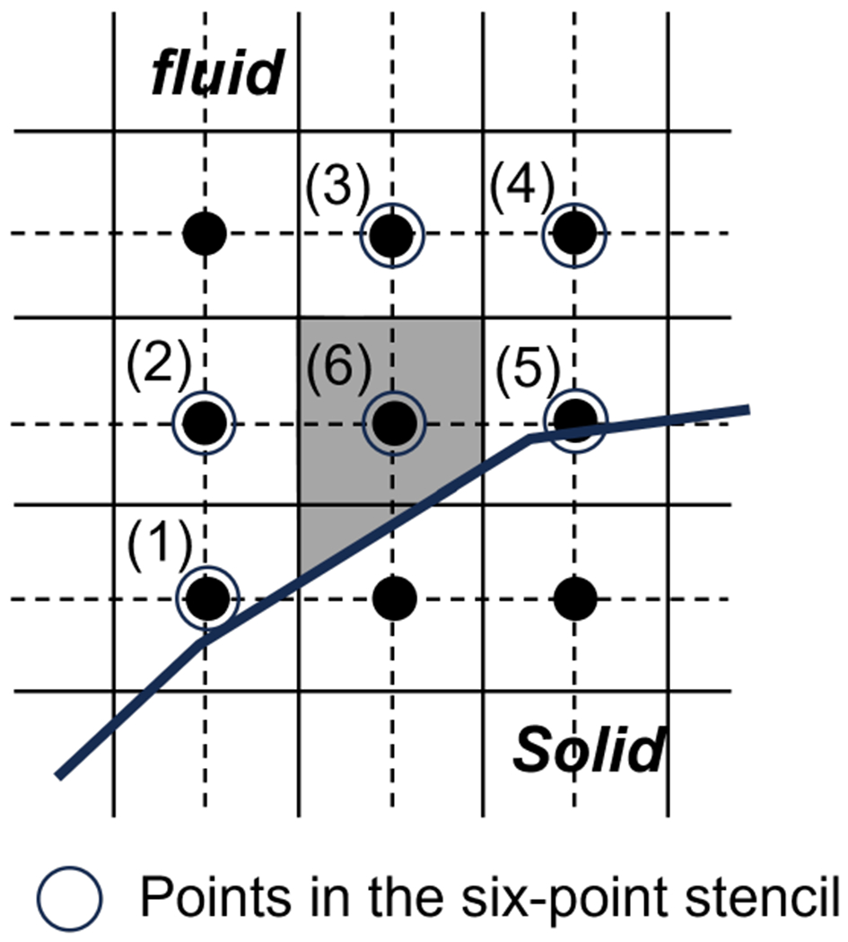
Figure from Ye et al. [55] depicting the cut-cell methodology, including the nodes employed to implement boundary conditions on the immersed boundary to 2^nd-order accuracy by using a two-dimensional polynomial interpolation. Reproduced from Ref.[55] with permission from Elsevier.

2. Ghost-Cell Based Methods

Within the category of discrete forcing methods are also methods that employ ‘ghost-cells’ (see Fig. 5) to impose the boundary conditions on the immersed boundary. Using a layer of cells immediately outside the computational boundary to impose external boundary conditions is a well-established procedure in many BCG codes [77–79]. This idea has been adopted as a way of imposing boundary conditions on immersed no-slip boundaries in body-nonconformal grid codes [71–73, 76, 80] as well as for multi-fluid interfaces [81, 82]. These ghost-cell approaches are typically based on finite-difference methods and do not reshape boundary cells. Instead they introduce an auxiliary equation for the ghost-cells that enforces the boundary condition on the immersed boundary, and this equation is coupled to the variables in the flow adjacent to the immersed boundary. The variable value on the ghost cell (GC) is determined by a 2^nd-order interpolation using the boundary condition on the ‘body-intercept’ (BI) point and the flow variable interpolated on the ‘image-point’ (IP).

FIG. 5.

Schematic of sharp-interface methodology of [73] that implements a 2^nd-order boundary condition on the immersed boundary using ghost-cells. Reprinted from Ref.[73] with permission from Elsevier.

The ghost-cell method (GCM) can also be extended to higher orders. In the work of Seo and Mittal [83], the ghost-cell value is obtained from an n-th order approximating polynomial interpolation by using an arbitrarily large number of stencil points around the immersed boundary (see Fig. 6). This high-order GCM has been employed for the wave propagation [83, 84] and compressible flow problems [85].

FIG. 6.

Schematic of the high-order ghost-cell method of Seo & Mittal [83]. The ghost-cell value is obtained from n^th-order approximating polynomial interpolation by using arbitrary number of stencil points around the immersed boundary in the range of R.

3. Pros and Cons

Since discrete forcing methods do not employ a Dirac-δ function, there is no need for regularization, nor is there the need for any ad-hoc forcing parameters such as in [36] and [50]. This avoids the boundary diffusion that results from the regularization of the Dirac-δ function and also obviates the compromise between accuracy and numerical stability that is required in these methods [36]. This also allows these methods to more easily achieve higher than first-order accuracy.

The cut-cell method is the one IBM that allows for strict discrete conservation of mass and momentum [55] but as pointed out earlier, higher-order conservation properties have been embedded into finite-difference based ghost-cell IBMs as well [76]. Cut-cell methods though have their own disadvantages: an increased complexity that is particularly severe for 3D problems [75], as well as the issue of ‘small cells’ [55]. Finally, discrete forcing methods also have to contend with the issue of ‘fresh cells’ for moving boundary problems [76]. Fresh cells are computational cells that emerge from the solid into the fluid due to the movement of the body on the stationary grid and the temporal discretization of the governing equations for these cells is problematic. Continuous forcing methods experience neither of the above problems due to the diffuse nature of the interface.

VI. SHARP-INTERFACE IB METHODS

The ‘diffuse’ and ‘sharp’ interface terminology in IBM originates from the physics of interfaces between two fluids [86, 87] but translating these notions into a precise definition for what constitutes a sharp-interface IBM is challenging. When an IBM method is labeled as a “sharp-interface” method, the implication is that the method applies boundary conditions on the immersed boundary with the same level of accuracy and precision as an equivalent BCG method.

This equivalence to BCG methods (see Fig. 7) can be distilled down to the following set of conditions for sharp-interface IBMs:

1. The imposition of no-slip, no-penetration boundary conditions is at a set of discrete points located precisely on the immersed boundary and nowhere else within the flow domain.

2. The spacing and resolution of these boundary points aligns with the underlying fluid grid.

3. The boundary conditions on these boundary points is imposed with an accuracy that is consistent with the underlying numerical scheme employed.

4. All grid points/cells in the flow domain impose the “native” governing equation, i.e. the Navier-Stokes equation, and not any other augmented or auxiliary equation.

5. The governing equations of flow are not solved inside the immersed body.

FIG. 7.

Schematic of a (A) curvilinear body-fitted grid and (B) Cartesian grid and cut-cells around a curved boundary

A. Categorization of IB Methods

All continuous forcing methods such as those of Peskin [1] and Goldstein et al. [36] as well as the fictitious domain [88] and front tracking methods [48] are diffuse-interface methods since they do not satisfy any of the conditions enumerated above.

Cut-cell methods [54–56, 75] are unequivocally sharp-interface methods since they clearly satisfy the above conditions. In fact, the cut-cell method can be viewed as a body-conformal finite-volume method where the finite-volumes are Cartesian everywhere in the domain except at the boundary, where they assume non-Cartesian shapes (see Fig. 7B).

Discrete forcing methods such as the ghost-cell methods of Tseng and Ferziger [71], Ghias et al. [72], Mittal et al. [73], Seo and Mittal [76], embedded boundary methods of Balaras and others [61, 74, 89, 90], immersed interface based methods [70] and the level-set based Cartesian grid methods of Udaykumar and co-workers [60, 91] satisfy the above conditions, and therefore function as sharp-interface methods. In fact, most if not all of these above mentioned methods impose the velocity boundary conditions on the immersed boundary with local 2^nd-order accuracy, which is higher than that needed to ensure global 2^nd-order accuracy and in doing so, provide high resolution to the boundary layers that develop on the immersed surfaces. The sharp-interface method of Seo and Mittal [76] even incorporates regional discrete conservation via a virtual cut-cell method, which further improves the accuracy of boundary layer flows.

All discrete forcing methods do not however satisfy the five conditions enumerated above. For instance, the mask method [34] spreads the discrete force over a layer of grid cells and is therefore a diffuse-interface method. Another exception is that of the so-called “stair-step” or “stair-case” method [92]. In this discrete forcing method, the immersed boundary is represented by a stair-step shaped surface that conforms to the underlying Cartesian grid. This method does not satisfy the first condition enumerated above, and consequently, is not a sharp-interface method.

The fifth condition seems innocuous but it has important implications for IB methods. This condition is generally associated with the fact that some IB methods (such as all the continuous forcing methods, and most penalization methods) do not impose an explicit boundary condition for pressure on the immersed surface and consequently, have to compute the pressure and the velocity everywhere on the grid including the region inside the body. This can significantly reduce the computational cost of the simulation since the inclusion of a boundary condition for pressure on the immersed surface can significantly amplify the computational effort for solving the pressure Poisson equation.

In the context of the fractional-step method, which is the standard choice for these solvers, the slip and penetration on a surface at the end of the pressure correction step is $O\left[{\left(\text{Δ}t\right)}^m\partial p/\partial \tau \right]$ and $O\left[{\left(\text{Δ}t\right)}^m\partial p/\partial n\right]$ respectively, where m is the order of the fractional step method and τ and n are the directions tangential and normal to the immersed body. For standard fractional-step schemes, m = 1, but second-order implementations [93] also exist. In BCG methods, it is standard to apply $\partial p/\partial n=0$ on all boundaries since it is consistent with the fractional-step method [94, 95] and this results in satisfaction of no-penetration to machine zero at the end of the time-step irrespective of the size of the time-step $\text{Δ}t$ as well as the magnitude of the normal pressure gradient. The latter can be large, especially in regions where the flow impacts normal to the body. All the discrete forcing methods described in the third paragraph of this section explicitly impose the Neumann condition for pressure on the immersed boundary and this allows them to enforce no-penetration to machine zero at the boundary points at the end of the time-step. This also decouples the grid points inside the immersed body from those outside, and eliminates the need to solve for the flow variables inside the body.

As pointed out in the previous paragraph, penalization methods, at least in their classic form, do not satisfy the fifth condition. The method of Fadlun et. al. [51] satisfies the first three conditions but not the fourth and fifth. We note however that the five conditions for sharpness enumerated earlier in this section may neither be necessary nor sufficient for generating high quality results from IBM simulations. This is because other factors such as the accuracy and dissipative nature of the spatial discretization scheme [96], and the choice of temporal discretization may be entangled with any specific implementation of IBM in a way as to impose additional constraints on its accuracy and fidelity.

B. Predictions from Sharp and Diffuse Interface Methods

Udaykumar and co-workers [97, 98] conducted a systematic head-to-head comparison of sharp-interface and diffuse-interface methods. They examined the effect of the interface treatment for flow Reynolds numbers ranging from O(100) to O(1000) and noted that the diffuse-interface method provided better prediction of drag on relatively coarse grids, but the sharp-interface method was more accurate on fine grids. This is not surprising given that on a sufficiently coarse grid, a lower-order method can have a lower absolute truncation errors than a higher-order method. The authors also found that diffuse-interface IBM under-predicted the surface vorticity on all grids and this was a consequence of the regularization of the forcing term.

The generality of the above conclusions, which are necessarily based on specific implementations of interface treatments, remains to be fully established. However, the experience of the current authors with other variants of the sharp-interface method [55, 73, 76, 83] is consistent with the above observations. Accurate prediction of surface vorticity, especially for higher Reynolds number flows where instabilities and transition to turbulence may occur, as well as the general equivalence to BCG methods are, in our view, the primary advantages of sharp-interface methods over their diffuse counterparts.

C. Are Sharp Interface IB Methods ≡ Body Conformal Grid Methods?

If sharp-interface IB methods satisfy the five conditions that derive from BCG methods, are there any differences between sharp-interface IB methods and BCG methods that have implications for the numerical accuracy of the flow near the immersed boundary? In our experience, there are some subtle issues that bear pointing out and we do this with reference to Figure 7, which shows schematics of a notional BCG as well the second-order cut-cell grid of Ye et al. [55] for a curved boundary. We choose the cut-cell method for comparison since as pointed out earlier, this is the IBM that is closest in its implementation to a BCG method.

The first difference to note is that while the shapes and sizes of the cells/finite volumes adjacent to the boundary generally vary smoothly for the BCG, for the cut-cell method, the finite-volumes can vary discontinuously for boundary cells in regions where the boundary crosses a layer of Cartesian grid points. This discontinuous variation in local boundary discretization is symptomatic not just of cut-cell methods but of all IB methods. As the boundary layer encounters these cells, it can affect the variation of surface quantities such as surface shear and pressure. Fortunately, this variation in the size of the cell is however limited to between ±50% of a nominal cell, and this boundary cell “unsmoothness” typically occur only for a small fraction of the cells in the entire domain.

Grid unsmoothness starts to manifest its impact primarily when the gradients within the boundary layer lack proper resolution. This issue becomes particularly pronounced in scenarios characterized by complex boundary conditions, and is accentuated by under-resolved wall processes—such as reacting flows, multiphase flows, radiation transport, and surfactant models. Addressing these challenges in the immersed boundary method (IBM) might necessitate case-specific adjustments. For instance, while wall models for turbulence can be incorporated within the IBM framework [99, 100], this process might not be as straightforward as it is for BCG methods.

One solution for IB methods is to increase the resolution in the boundary region, but this is not always feasible. Another well-known technique to enhance solution quality in cases of marginal resolution is the imposition of discrete conservation. In the context of IBMs, cut-cells [55, 56, 75] or “virtual” cut-cell [76] methods provide discrete conservation and lead to improvements in solution quality.

We observe that BCG methods are not entirely impervious to the influence of grid unsmoothness. Instances of discontinuous variations in the boundary cells can manifest due to inherent grid irregularities. This phenomenon is particularly notable in regions characterized by significant surface curvature, corners, branch-cuts, or other intricate topological transitions.

Another difference between BCG methods and sharp-interface IBMs is for problems with moving or deforming boundaries. For such problems, IBM methods encounter the so called “fresh cell” problem [56, 73], where cells that were inside the body at one time-step emerge into the fluid at the subsequent time-step. For sharp-interface IBMs, these fresh cells do not have a valid time-history and one has to temporarily employ some space-time interpolation [73] or cell-merging [56] to advance the equation in time for these cells. For the small number of fresh-cells that typically emerge at a given time-step, this can reduce the local accuracy of the solution.

BCG methods such as ALE employ deforming meshes coupled with time-evolving control-volume formulations and do not have the fresh-cell problem as long as the movement of the boundary is limited. Once the boundary motion is large enough so as to require a local and even a global remeshing [101, 102], ALE methods also have to resort to interpolation schemes for the remeshed cells in order to advance the governing equation for these cells. Thus, while the fresh-cell problem in sharp-interface IBM is limited to a few boundary cells, it can occur on a much larger scale for ALE methods.

IBMs also have a subtle advantage over conventional BCG methods that in our view, is not fully appreciated. It is well known that grid skewness (i.e. nonorthogonality in the shape of cells) generates additional dissipation and dispersion errors that have the potential to affect the evolution and advection of vortex structures, waves and turbulence on the grid [103]. The use of Cartesian grids eliminates this additional source of error in IBM simulations and enhances the ability of IBM methods to more accurately simulate turbulent flows.

VII. GALLERY OF IBM SIMULATIONS

Applications of IBMs span virtually all scientific and engineering domains in fluid mechanics and it is not possible to summarize this vast literature here. Instead, we present eleven curated cases that demonstrate not only the unique capabilities of IBM methods but also the accuracy and fidelity of these methods. While four examples are from our own work, case-studies from other research groups are also included in order to highlight the diversity of IBM approaches and their applications.

A. Simulation of Fish Swimming in a School

This is a direct numerical simulation of a school of nine fish swimming with prescribed carangiform kinematics [104] against an incoming flow. The Reynolds number based on the tail-beat frequency(f) and the body length(L) is $Re=f{L}^2/\nu =5000$. Simulations are performed using our sharp-interface incompressible immersed boundary flow solver (ViCar3D) [73, 76] on a fixed non-uniform Cartesian grid (See Fig. 8A) with a total of 54 million grid points and Fig. 8B shows the vortex structures generated by the school. Figure 8C shows the time-averaged net force in the surge direction generated by each fish normalized by the mean thrust for a single fish, and we note that for the tail-beat phase and inter-fish distance chosen for this case (which is based on an earlier investigation of two fish by Seo and Mittal [104]), most fish in the school experience an increase in net surge force due to the hydrodynamic interactions with the wakes of upstream fish.

FIG. 8.

Direct numerical simulation of a school of 9 fish. A: Fish school model immersed in the Cartesian grid. B: 3D vortical structures. C: Net force in the surge direction normalized by the mean thrust of a single fish. Number indicates individual fish in the school shown in B. Figure provided by Ji Zhou.

This case is shown primarily to highlight the complexity of the flow configurations and immersed bodies that can be handled by IBMs. Simulation of such a flow that contains multiple moving/deforming bodies and membranes (the caudal fin) in close proximity would represent a nearly insurmountable challenge for any BCG method. Indeed, the vast majority of computational studies of the fluid dynamics of swimming and flying employ IBMs because of this reason although there are some notable exceptions [105–108].

B. Effect of Dimple Shapes on Golf Ball Drag

It has been known that passive roughness such as dimples are effective in reducing the drag force on bluff bodies. A well-known example of this application is a golf ball and Smith et al.[109] performed direct numerical simulations of flow over a golf ball at a Reynolds number of 1.1 × 10⁵ by using a sharp-interface IBM. Beratlis et al.[110] investigated the drag reduction on spheres by tessellation using the IBM. Figure 9A shows the vortex structure for a ball with tessellated dimples at Re=1.1 × 10⁵. A 1100 × 1500 × 3000 point grid was used in this simulation, and each dimple on the sphere was resolved by 40 × 50 × 70 grid points. The simulation ran on 1500 CPU cores for 2 weeks and the drag coefficients obtained from the IBM simulations were in good agreement with the experiments (see Fig. 9B).

FIG. 9.

A: Isosurface of the Q-criterion visualizing vortical structures near the top of the tesselated sphere at Re=1.1 × 10⁵. B: Drag coefficient versus Re for three different golf balls, with dimples, tessellated with 162 polyhedron faces, and 192 faces. Wind tunnel measurements are shown with solid line and DNS values are shown with dots. Figures provided courtesy of Dr. Elias Balaras.

Other examples of IBM based simulations of high Reynolds number bluff body wake flows with validation against experimental data are by Meyer et al. (Re=3900 flow past a cylinder) [70] and Xu et al. [111] (flow past a sphere at Re=3,700-10,000). Data from compressible flow IBM simulations of bluff-body wakes flows is also highlighted later in this section.

C. Turbulent Boundary Layer over Sharkskin Denticles

Boomsma and Sotiropoulos [112] performed direct numerical simulations of flow over sharkskin denticles in turbulent channel flow using a sharp-interface IBM[113]. A representative denticle from Isurus oxyrinchus (short-fin Mako) was scanned using micro-CT and a total of 324 individual denticles were used to cover the channel wall. In the baseline simulation, the Reynolds number based on the bulk flow velocity was Re = 2800 (Re_τ = 180), and about 130 million grid points were used to resolve the turbulent flow over the surface covered by the denticles. Figure 10 shows a close-up view of the flow field around the denticles. The denticles were found to increase the total drag on the wall (see Fig. 10), and the change in drag force due to the denticles compared reasonably well to the experimental measurement [114].

FIG. 10.

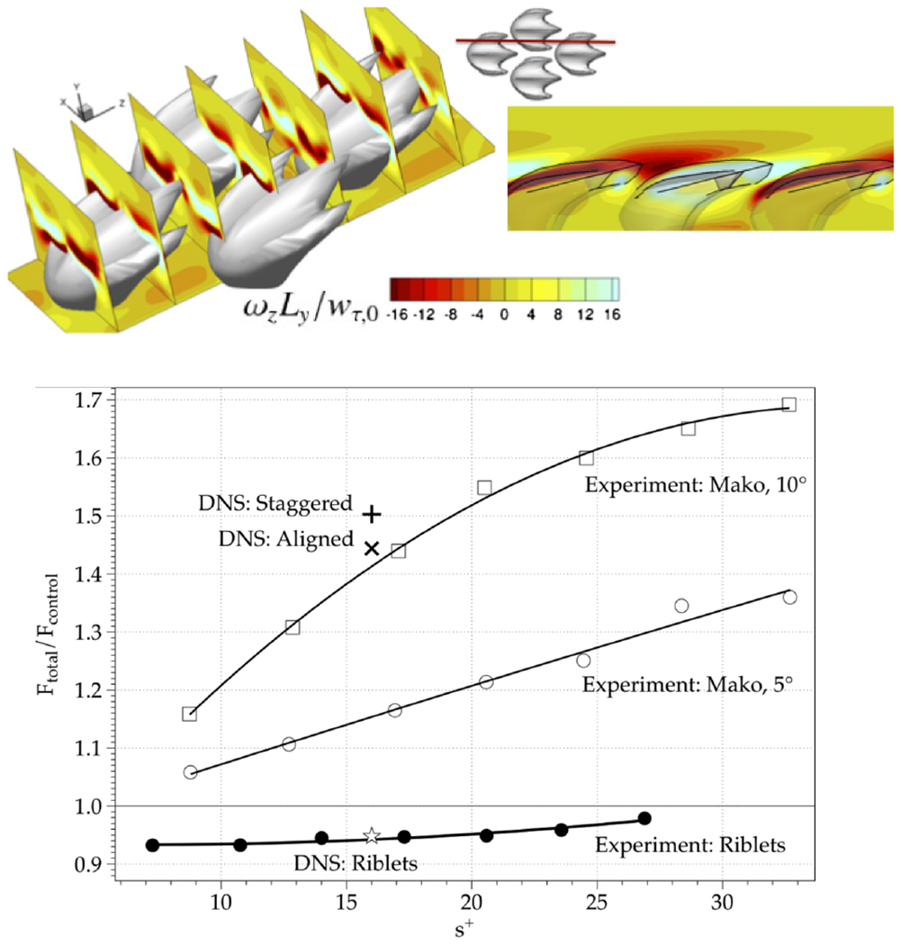
Direct numerical simulation of a turbulent boundary layer at Re_τ = 180 over a surface with modeled sharkskin denticles using a sharp-interface IBM [112]. Top figure shows views of mean streamwise vorticity for a staggered arrangement of denticles. Inset shows the spanwise location of side view. Bottom figure shows the ratio between total drag with and without sharkskin (and with/without riblets) from the present DNS. Fitted curves, open squares/circles, and filled circles are experimental data. The + and × mark IBM based DNS data for the staggered and aligned denticle cases, respectively. The open star is the IBM based DNS result for the riblets. Reprinted from Ref.[112] with the permission of AIP Publishing.

IBM based simulations of transitional and turbulent wall bounded flows with and without complex surface geometries have also been simulated in several other studies; see for instance Refs. [115, 116].

D. Flight Aerodynamics of a Hummingbird

Figure 11 shows the simulation of humming bird hovering performed by Song et al. [118]. 3D high-fidelity wing kinematics of hummingbird hovering was reconstructed from high-speed videos and was used as input for simulation of the unsteady aerodynamics of a hovering hummingbird. As shown in Fig. 11A, the 3D model of hummingbird was immersed in the Cartesian grid, and the flow simulation was done by a sharp-interface IBM [119]. The flow Reynolds number based on the average wingtip velocity was 3000 and a total of 30 million grid points were used to resolve the flow field. For the validation of the simulation, the phase-averaged circulation around the wing was compare with the experiment data of Warrick et al. [117], and Fig. 11C shows that the circulation at 50% wingspan matches reasonably well with the experimental data.

FIG. 11.

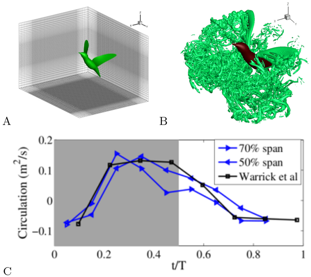
IBM simulation of hummingbird hovering. A: 3D kinematic model of hummingbird immersed in the Cartesian grid. B: Three dimensional vortical structures in the flow. C: Comparison of circulation around the wing with experiment of Warrick et al. [117]. Figures provided courtesy of Dr. Haoxiang Luo.

Other examples of IBM simulations in the arena of biolocomotion that have been verified against experiments are those for a hovering moth [120], a pectoral fin of a fish [121].

E. Impact of a Sphere with an Elastic Membrane in Fluid

This case highlights the ability of IB methods to model complex fluid-structure interaction (FSI) problems. Verzicco and Querzoli [61] analyzed the impact of a rigid spherical pendula impacting on rubber membranes (Fig 12A) in a fluid at different Reynolds numbers to understand the contact dynamics in deformable bodies in a viscous fluid. They investigated the problem both by laboratory and numerical experiments (Fig 12B) and a developed a new contact model to perform the simulations. The simulations were carried out using the sharp-interface IB method of De Tullio and Pascazio [90]. Simulations employed grids with O(100) million grid points and Reynolds numbers extended up to 1000. They found that the collision dynamics depended on many parameters, the most important ones being the impact Stokes number and the ratio of the membrane thickness-to-sphere diameter. Extensive comparisons were made with the experimental results (Fig 12C) and the simulations were found to accurately predict the features of the impact on the sphere and the membrane.

FIG. 12.

A: Schematic of the problem configuration. B: (upper) Experimental visualisations of the pendulum approaching the membrane.(lower) Numerical results for Re=1000 of the vertical velocity component overlaid with velocity vectors in the symmetry y–z-plane. The thin solid line shows the computed membrane profile. C: Comparison of numerical (symbols) and experimental (line) time evolution of the vertical coordinate of the pendulum centre for a membrane for a selected case. Figures provided courtesy of Dr. Roberto Verzicco.

Other studies involving IB simulations of FSI problems with verification against experiments can be found in the literature (see for instance Refs. [122–124]) and the interested reader is referred to the review article of Griffith and Patankar [125] for a comprehensive discussion on this topic.

F. Generation of Wing Tones by Flying Mosquitoes

Multiphysics modeling such as the FSI modeling shown in the previous section, is a particular strength of IB methods. In this subsection, as well as the next, we show two additional examples of multi-physics simulations done using IBMs.

Seo et al. [126] studied wing tone generation by mosquitoes using the IBM flow simulation coupled with aeroacoustic sound prediction based on the Ffowcs Williams and Hawkings (FW-H) equation [127]. Figure 13A shows the instantaneous vortical structure around the flapping mosquito wing at the phase of peak lift during down stroke. The wing tone was then predicted by the FW-H equation with the time dependent surface pressure data obtained from the flow simulations. Figure 13B shows 3D sound pressure level (SPL) directivity pattern. The predicted wing tone compared well with the measurement of Arthur et al. [128].

FIG. 13.

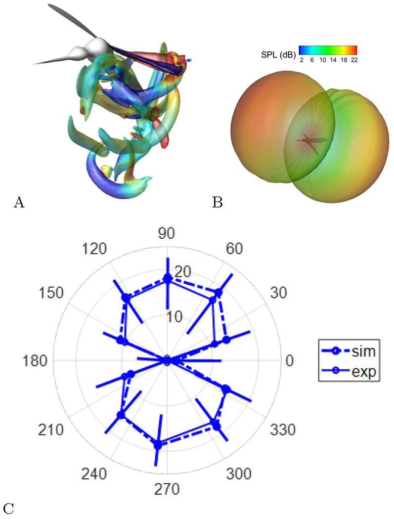
Prediction of wing tones by a flying mosquito. A: Vortex structures around flapping wing of mosquito resolved by the IBM simulation. B: 3D sound pressure level (SPL) directivity pattern for the fundamental wing beat frequency at 10 cm distance. C: Comparison of SPL directivity on the coronal plane at 10 cm distance. sim: Prediction form the simulation. exp: Experimental measurements by microphone arrays. Error bars denote cycle-to-cycle variation.

In order to further validate the computational methods, a joint experimental-computational study has also been performed [129]. In the study, tethered mosquitoes were imaged via a high-speed video camera and the wing tone sounds were recorded by a microphone array. Simulations of the flow and acoustics were carried out with the wing kinematics extracted from the experiments and Fig. 13C shows the wing tone SPL directivity on the coronal plane at 10 cm distance for the fundamental wing-beat frequency. The agreement between the experimental measurements and the predictions from the simulations was found to be excellent, indicating the fidelity of the IBM based aeroacoustic modeling approach.

G. Heart Murmurs Generated by Turbulent Flow in the Aorta

This case is specifically for the heart murmurs generated by a valvular constriction [84] in the human aorta but it generally relates to structural acoustics associated with turbulent wall pressure fluctuations such as in hydroacoustic noise [130].

The in-vitro model consisted of a stenosed tube embedded inside a cylinder made of a tissue mimicking viscoelastic material (see Fig. 14A, middle). The flow through the tube, which was at a Re_D = 4,000, transitions to turbulence downstream of the constriction and generates wall pressure fluctuations which subsequently generate acoustic waves that propagate through the surrounding viscoelastic material to the surface. Surface measurements of the acoustic wave for this set-up were conducted in an anechoic chamber with a contact microphone (BIOPAC) and an accelerometer (HP).

FIG. 14.

A: Modeling of heart murmur generated by a constriction in an artery. (Left): Schematic of the set-up Turbulent flow in the stenosed tube embedded within a tissue mimicking viscoelastic cylinder (Middle): Turbulent flow in the stenosed tube. (Right): Elastic waves in the viscoelastic media resolved by the simulation. B: Comparisons between the simulation results and the experimental measurements. (Left): Frequency spectra of radial accelerations measured on the outer surface of gel material. Exp-BIOPAC: measurement by BIOPAC contact microphone, Exp-HP: measurement by HP accelerometer. (Right): Variation of spectral energy of the signal for three different frequency bands; solid line with filled symbol: simulation; dashed line with hollow symbol and error bar: experimental measurement.

The configuration was modeled computationally with a sharp-interface incompressible immersed boundary flow solver (ViCar3D) [73] coupled with a high-order, sharp-interface immersed boundary solver for acoustic wave propagation [84] in viscoelastic media. Figure 14A shows the turbulent flow structures in the stenosed tube as well as the elastic waves generated in the surrounding viscoelastic medium by the wall pressure fluctuation. The comparison of the surface fluctuations between the simulations and experiment (Fig. 14B) showed excellent agreement over a wide range of frequencies and spatial location [84]. This study showcased the ability of the sharp-interface IB approach to not only predict turbulent wall pressure fluctuations but also the multiphysics problem of flow-noise and acoustic wave propagation.

H. Flow Past a Caudal-Fin Inspired Pitching Panel

Figure 15 shows the simulation of flow past a pitching panel at Re=10,200 and Strouhal number of 0.27. The panel was sinusoidally pitched with a peak-to-peak amplitude of 15°. The simulation was carried out by Zhang et al. [131] using a sharp-interface immersed boundary method with local grid refinement. The computational domains with different refinement levels and baseline Cartesian mesh are shown in Fig. 15A. To resolve the flow structures at this high Reynolds number, two layers of refined mesh blocks were employed, and the finest resolution around the panel was 0.0052C (C is the chord length of the panel). The total number of grid points used was around 15.4 million. The comparisons of computed wake structures against the PIV measurements of King et al. [132] are shown at two time-instances in the pitching cycle in Fig. 15B, and the simulation results were found to match very well with the experiment.

FIG. 15.

Simulation of flow past a pitching panel at Re=10,200 and Strouhal number of 0.27 carried out by Zhang et al. using a sharp-interface immersed boundary method [131]. Comparison of the computed wake against the experiments of King et al. [132] are shown at two time-instances in the pitching cycle. Figures provided courtesy of Dr. Haibo Dong.

I. High-Speed Wake Flows

Figures 16 & 17 show the results of a high-order sharp-interface IBM (ViCAS3D [85]) applied to compressible flows. The simulation of flow past a circular cylinder at Re = 200, 000 and flow Mach number, M = 1.7 is shown in Fig. 16. A sharp-interface IBM with high-order polynomial interpolation [83] was used and the cylinder diameter was resolved by 400 grid points. Density gradient magnitude contours shown in Fig. 16A indicate various flow features typical of a high speed compressible flow including bow, separation, and oblique shocks. The pressure coefficient (C_p) on the cylinder surface computed from this IBM simulation is compared with the results from other BCG as well as IBM simulations in Fig. 16B and found to match reasonably well.

FIG. 16.

Flow past a circular cylinder at Re = 200, 000 and flow Mach number, M = 1.7 using the code described by Turner et al.[85] A: Density gradient magnitude $\left|\nabla {\rho }^{\ast }\right|$ produced by a circular cylinder. B: Comparison of cylinder pressure coefficient C_p with other simulation results. IB: Immersed Boundary, URANS: Unsteady Reynolds Averaged Navier-Stokes, DNS: Direct Numerical Simulation. Figure provided by Dr. Jacob Turner.

FIG. 17.

Flow past a sphere at Re = 50, 000 and flow Mach number, M = 4.0. Flow field at an early time in the flow development visualized by Q-criterion colored by streamwise vorticity with the temperature contours shown in the z/D = 0 plane. Figure provided by Dr. Jacob Turner.

Figure 17 shows the simulation of flow past a sphere at Re = 50, 000 and M = 4.0. A total of 90 million grid points were used in this simulation. A bow shock in front of the sphere and complex vortex structures in the wake are clearly visible. The drag coefficient obtained from the simulation was 0.98, which is within 6% of the reported value 1.04 [133].

Other compressible flow simulations using IBM that have been verified against experiments or BCG methods are by De Tulio et al. [134], Nam & Lien[135], Al-Marouf & Samtaney [136], and Mao et al. [137].

J. Shock-Void Interaction

IB methods have been applied to a variety of compressible multiphase and multimaterial flows. Figure 18 shows the collapse of a void pore in the polymethyl methacrylate (PMMA) medium by the interaction with the shock wave at 2.3 km/s which was simulated by the sharp-interface IBM based multi-phase flow solver SCIM-ITAR3D [138, 139]. The interface was represented via level sets and resolved by a ghost-fluid method. Figure 18A shows a three dimensional void interface and temperature contours on the cross section, and the evolution of the void interface is found to compare reasonable well with experimental measurements (Fig. 18B).

FIG. 18.

Simulation of shock-void interaction. A: Instantaneous Void interface and temperature contours on the cross section. B: Time evolution of void interface compared with experimental measurement. Black: Experiment. Blue: Simulation. Figures provided courtesy of Dr. H. S. Udaykumar.

K. Wall-Modeled LES of Hypersonic Ramp Flow

The final case presented in this section is of a wall-modeled large-eddy simulation of a hypersonic turbulent boundary layer traversing a compression ramp. The Reynolds and Mach numbers for the flow are 1.89 × 10⁷ and 7.2 respectively. The finite-difference method employed here has a spatial accuracy that ranges between 2^nd and 3^rd order and the IB method implemented in the solver employs ghost-point based interpolations to impose the boundary conditions. As pointed out earlier, sharp-interface methods experience localized grid discontinuities in the boundary cells and these can be particularly important in scenarios characterized by complex boundary conditions and the implementation of wall-models for turbulence can be more difficult than for BCG methods. This case therefore addresses both of these challenges.

The results in the Fig. 19 as well as the other test cases in this study suggest that wall-modeled LES with IBMs can provide reasonable results, but the authors noted the need for particular attention to the numerical accuracy and dissipation characteristics of the numerical treatment near the wall.

FIG. 19.

Results from IBM wall-modeled LES of hypersonic flow over a 8° compression corner by van Noordt et al. [100] Top left: schematic diagram for the compression corner case. Top right: instantaneous flow field visualization for the test case showing isosurfaces of temperature colored by the streamwise velocity. Bottom: Comparison of surface quantities Stanton number (left), skin friction coefficient (right) against DNS. Reproduced with permission from author William van Noordt.

VIII. FREQUENTLY ASKED QUESTIONS

In this section we address some of questions that come up frequently regarding the capabilities of IBMs. These questions provide a practical and useful context for comparing IB and BCG methods in CFD.

A. Can IB methods compute boundary layer flows accurately?

The implicit assumption underlying this query is that all IBMs (Immersed Boundary Methods) are diffuse-interface approaches incapable of enforcing boundary conditions with the same level of precision as BCG (Boundary-Conforming Grid) methods. Consequently, they are believed to fall short in accurately capturing boundary layers. Nevertheless, as succinctly summarized earlier, the past two decades have witnessed a predominant shift in the realm of IBMs towards sharp-interface methodologies with second-order (and even higher - see Refs. [83, 140] for examples) levels of both local and global accuracy. These advanced techniques deliver a degree of precision and exactitude in boundary layer resolution that mirrors the capabilities of BCG methods (as discussed in Section VII). Indeed, beyond the few examples showcased here, there exist several studies where sharp-interface IBMs have been used to accurately predict the evolution of boundary layers on complex surfaces, thereby answering the above question in the affirmative.

B. Can IB methods simulate flows at high Reynolds numbers?

Given that away from the immersed boundary, the discretization of IB methods is similar to that of BCG methods, the question at hand implicitly concerns the ability of IBMs to accurately resolve flow in the vicinity of the immersed body at high Reynolds numbers. As mentioned in the preceding paragraph, sharp-interface methods possess capabilities akin to BCG methods in resolving boundary layers. Therefore, simulating high Reynolds number flows hinges on the capacity to increase the resolution within the boundary layers.

BCG methods generally allow for a finer resolution perpendicular to the wall with a level of precision that is typically not attainable with the Cartesian grids commonly employed in IBMs. As highlighted by Mittal and Iaccarino in their work [66], this discrepancy results in a more rapid increase in grid size with Reynolds numbers for IBMs compared to BCG methods. Curvilinear as well as unstructured and overset grid methods however, have a much higher operation count per grid point than IB methods. This is because they have significantly larger number of terms in the equations, and the condition-number of discretized operators can also be larger, resulting in slow convergence. Thus, a larger grid for IB methods does not necessarily imply an equivalently larger CPU time for the simulations. Second, for immersed boundaries with geometrical complexities such as high curvatures, corners and junctions, BCGs can also have difficulties in imparting high resolution that is limited to only the boundary layer regions while maintaining grid quality.

Finally, the use of local-grid refinement [131, 134, 138, 141, 142] allows IB methods to provide high resolution in regions around the immersed body in a more selective manner and but it diminishes the structured nature of the mesh and has implication for the convergence of the sparse systems that result from the discretization. In the previous section we have provided examples and references for many studies for high Reynolds number flows where IB methods have generated verifiable results, including surface related quantities such as pressure and drag.

The question in the end comes down to IBM’s computational efficiency compared to the BCG method. Such comparisons are complex due to various factors like solver selection, test-case choice, and computing hardware. One such study along these lines was by Capuano et al. [143] who compared three solvers for simulating flow over a Re = 3700 sphere: Nek5000 (a high-order spectral-element code), OpenFOAM (a general-purpose unstructured finite-volume solver), and their inhouse Cartesian IBM solver. The study indicated that Nek5000 and IBM performed similarly in terms of cost-effectiveness for global and local flow properties. Conversely, OpenFOAM required significantly more degrees-of-freedom (and higher cost) to match key features like the downstream recirculation bubble length. At finer resolutions, the three codes closely agreed on most flow metrics. The authors concluded that high-order methods and second-order, energy-conserving IBM approaches are viable for high-fidelity simulations of turbulent flows with separation. Similar comparisons for other complex geometries and moving boundary problems would go a long way in providing informing CFD practitioners about the computational costs of IBM simulations.

C. Can IB methods resolve turbulent flows?

As with the previous question, this question also relates to the ability of IBMs to resolve turbulent flows that occur in the vicinity of immersed boundaries. As outlined in the previous two paragraphs, the numerical accuracy and fidelity of sharp-interface IB methods is similar to standard BCG methods, thus the question really boils down to the ability of IB methods to provide adequate resolution near the immersed boundary to resolve turbulence.

In order to examine this question, it is useful to consider two relevant resolution requirements for DNS of canonical attached turbulent boundary layers. The first is that the grid resolution requirement at the wall be $\left(\text{Δ}{x}^{+},\text{Δ}{y}^{+},\text{Δ}{z}^{+}\right)\approx \left(12,0.1,7\right)$ [144], which implies a grid aspect-ratio near the wall of roughly 120:1:70. Second, the wall-normal grid size can increase by a factor of about 50 in the outer regions of the turbulent boundary layer. BCG methods can potentially take advantage of these requirements by employing grids that are highly non-isotropic $\left(\text{Δ}x;\text{Δ}z\gg \text{Δ}y\right)$ near the wall, and which expand rapidly away from the wall. A state-of-the-art example of this is the CharLES code developed at the Center for Turbulence Research [145]. In IB methods on the other hand, since the underlying Cartesian grid is not necessarily aligned with the boundary, there is no easy way to fully exploit these resolution requirements. While local refinement techniques [131, 134, 138, 141, 142] can be used to take advantage of the second condition, most IB methods, even those that employ local-grid refinement, use isotropic grids, i.e. grids with $\text{Δ}x\approx \text{Δ}y\approx \text{Δ}z$, near the immersed boundary, and therefore do not exploit the first condition. Thus, for canonical turbulent flows, the size of the grid for IB methods is significantly larger than for a corresponding BCG method.

This difference between IB and BCG method however diminishes for geometrically complex boundaries, such as for rough walls [146] or for non-canonical turbulent flows such as those with separation [147, 148], since such flows require near-wall grids that are more isotropic. Indeed, several examples exist for such flows being simulated successfully with sharp-interface IB methods (see Ref. [99, 116, 149]) including those shown here [109, 110, 112]. In fact, for this class of turbulent wall bounded flows, the ability of IB methods to easily handle geometric complexity gives them, in our view, an edge over BCG methods. Similarly, IB method generally have an advantage in simulating turbulent flow with moving boundaries for all the reasons outlined in this article.

Incorporating Reynolds-averaged Navier-Stokes (RANS), wall-resolved LES, and wall-modeled LES into Cartesian grid IBMs may introduce certain added intricacies. However, these challenges are certainly surmountable, as evidenced by a range of successful implementations [99, 150–152].

Finally, as pointed out earlier, the lack of grid skewness related errors in IBM could be a significant advantage for these method over BCG methods, since vortices and turbulence structures away from the immersed boundary can be resolved and convected over Cartesian grids with higher fidelity than on non-orthogonal curvilinear grids.

D. Can IB method simulate high-speed flows?

In the context of IB methods, flow compressibility brings in a few additional aspects for consideration. These are the appearance of complex heat-flux boundary conditions at the surface associated with the energy equation, and the need to resolve shocks in the vicinity of the body. As pointed out by Mittal and Bhardwaj [153], the thermal boundary conditions for compressible flows have been incorporated in several different sharp-interface IB solvers. For example, using the ghost-cell based sharp-interface IBM, Dirichlet as well as Neumann type boundary conditions for arbitrary variables can be imposed on the solid surface/interface [83], which enables the incorporation of heat and mass flux boundary conditions necessary for the high-speed compressible flows [85]. There also exist several examples of simulations at high Mach numbers (see Figs. 16–19) and references in Mittal & Bhardwaj [153]) with IB methods that resolve shock-boundary layer interaction. Therefore, while addressing local numerical accuracy near the immersed body is paramount for high-speed compressible flows, this challenge is surmountable. Nonetheless, it’s imperative to recognize that these flows often occur at high Reynolds numbers, warranting consideration of the three additional issues delineated earlier in this section.

IX. CLOSING

This perspective piece on immersed boundary methods draws inspiration from the aphorism “Those who do not understand history may be forced to repeat it.” IB methods are increasingly becoming an essential tool for fluid dynamicists who are keen to attack flows problem in all their native complexity. Our hope is that by comprehending the historical trajectory of the advancements in these methods—why, when, and how they were developed—researchers are better prepared to critically evaluate these methods and empowered to innovate in ways that significantly advance the state-of-the-art in these methods.

References

- [1].Peskin CS, Flow patterns around heart valves: A digital computer method for solving the equations of motion, Ph.D. thesis, Albert Einstein College of Medicine of Yeshiva University, July 1972 (1972). [Google Scholar]
- [2].Fromm JE and Harlow FH, Numerical solution of the problem of vortex street development, Physics of Fluids 6, 975 (1963). [Google Scholar]
- [3].Harlow FH and Fromm JE, Dynamics and heat transfer in the von karman wake of a rectangular cylinder, Phys. Fluids 7, 1147 (1964). [Google Scholar]
- [4].Harlow FH and Welsh JE, Numerical calculation of time-dependent viscous incompressible flow of fluid with free surface, Physics of Fluids 8, 2182 (1965). [Google Scholar]
- [5].Viecelli JA, A method for including arbitrary external boundaries in the mac incompressible fluid computing technique, Journal of Computational Physics 4, 543 (1969). [Google Scholar]
- [6].Viecelli JA, A computing method for incompressible flows bounded by moving walls, Journal of Computational Physics 8, 119 (1971). [Google Scholar]
- [7].Amsden AA and Hirt CW, A simple scheme for generating general curvilinear grids, Journal of Computational Physics 11, 348 (1973). [Google Scholar]
- [8].Rizzi AW and Inouye M, Time-split finite-volume method for three-dimensional blunt-body flow, AIAA J. 1, 1478 (1973). [Google Scholar]
- [9].Gal-Chen T and Somerville RC, On the use of a co-ordinate transformation for the solution of the navier-stokes equations, Journal of Computational Physics 17, 209 (1975). [Google Scholar]
- [10].Hung TK and Brown TD, An implicit finite-difference method for solving the navier-stokes equation using orthogonal curvilinear coordinates, Journal of Computational Physics 23, 343 (1977). [Google Scholar]
- [11].Thames FC, Thompson JF, Mastin CW, and Walker RL, Numerical solutions for viscous and potential flow about arbitrary two-dimensional bodies using body-fitted coordinate systems, Journal of Computational Physics 24, 245 (1977). [Google Scholar]
- [12].Clark TL, A small-scale dynamic model using a terrain-following coordinate transformation, Journal of Computational Physics 24, 186 (1977). [Google Scholar]
- [13].Oden JT, Finite-element analogue of navier-stokes equation, Journal of the Engineering Mechanics Division 96, 529 (1970). [Google Scholar]
- [14].Cheng RTS, Numerical solution of the navier-stokes equations by the finite element method, Physics of Fluids (1958-1988) 15, 2098 (1972). [Google Scholar]
- [15].Taylor C and Hood P, A numerical solution of the navier-stokes equations using the finite element technique, Computers & Fluids 1, 73 (1973). [Google Scholar]
- [16].Thompson JF, Thames FC, and Mastin CW, Automatic numerical generation of body-fitted curvilinear coordinate system for field containing any number of arbitrary two-dimensional bodies, Journal of Computational Physics 15, 299 (1974). [Google Scholar]
- [17].Vinokur M, Conservation equations of gasdynamics in curvilinear coordinate systems, Journal of Computational Physics 14, 105 (1974). [Google Scholar]
- [18].Launder B and Spalding D, The numerical computation of turbulent flows, Computer Methods in Applied Mechanics and Engineering 3, 269 (1974). [Google Scholar]
- [19].Hirt CW, An arbitrary lagrangian-eulerian computing technique, in Proceedings of the Second International Conference on Numerical Methods in Fluid Dynamics, edited by Heidelberg SB (1971) pp. 350–355. [Google Scholar]
- [20].Hirt CW, Amsden AA, and L. CJ, An arbitrary lagrangian-eulerian computing method for all flow speeds, Journal of Computational Physics 14, 227 (1974). [Google Scholar]
- [21].Steger JL, Dougherty FC, and Benek JA, A chimera grid scheme, in Advances in Grid Generation: Presented at Applied Mechanics, Bioengineering, and Fluids Engineering Conference, Houston, Texas, June 20-22, 1983, Vol. 5, edited by Ghia KN and Ghia U (American Society of Mechanical Engineers, 1983). [Google Scholar]
- [22].Benek J, Buning P, and Steger J, A 3-d chimera grid imbedding technique. aiaa paper 85-1523, in 7th Computational Fluid Dynamics Conference, Cincinatti, OH (1985). [Google Scholar]
- [23].Peskin CS, Flow patterns around heart valves: a numerical method, Journal of Computational Physics 10, 252 (1972). [Google Scholar]
- [24].Peskin CS, Numerical analysis of blood flow in the heart, Journal of Computational Physics 25, 220 (1977). [Google Scholar]
- [25].McCracken MF and Peskin CS, A vortex method for blood flow through heart valves, Journal of Computational Physics 35, 183 (1980). [Google Scholar]
- [26].McQueen DM and Peskin CS, Computer-assisted design of pivoting-disc prosthetic mitral valves, Journal of Thoracic and Cardiovascular Surgery 86, 126 (1983). [PubMed] [Google Scholar]
- [27].McQueen DM and Peskin CS, Computer-assisted design of butterfly bileaflet valves for the mitral position, Scandinavian Journal of Thoracic and Cardiovascular Surgery 19, 139 (1985). [DOI] [PubMed] [Google Scholar]
- [28].McQueen DM and Peskin CS, A three-dimensional computational method for blood flow in the heart. ii. contractile fibers, Journal of Computational Physics 82, 289 (1989). [Google Scholar]
- [29].Fauci LJ and Peskin CS, A computational model of aquatic animal locomotion, Journal of Computational Physics 77, 85 (1988). [Google Scholar]
- [30].Fauci LJ, Interaction of oscillating filaments: a computational study, Journal of Computational Physics 86, 294 (1990). [Google Scholar]
- [31].LeVeque RJ, Peskin CS, and Lax PD, Solution of a two-dimensional cochlea model using transform techniques, SIAM Journal on Applied Mathematics 45, 450 (1985). [Google Scholar]
- [32].Beyer RP, A computational model of the cochlea using the immersed boundary method, Journal of Computational Physics 98, 145 (1992). [Google Scholar]
- [33].Dillon R, Fauci L, Fogelson A, and Gaver D I. I. I., Modeling biofilm processes using the immersed boundary method, Journal of Computational Physics 129, 57 (1996). [Google Scholar]
- [34].Briscolini M and Santangelo P, Development of the mask method for incompressible unsteady flows, Journal of Computational Physics 84, 57 (1989). [Google Scholar]
- [35].Angot P, Bruneau CH, and Fabrie P, A penalization method to take into account obstacles in incompressible viscous flows, Numerische Mathematik 81, 497 (1999). [Google Scholar]
- [36].Goldstein D, Handler R, and Sirovich L, Modeling a no-slip flow boundary with an external force field, Journal of Computational Physics 105, 354 (1993). [Google Scholar]
- [37].Saiki EM and Biringen S, Numerical simulation of a cylinder in uniform flow: application of a virtual boundary method, Journal of Computational Physics 123, 450 (1996). [Google Scholar]
- [38].Clarke DK, Hassan HA, and Salas MD, Euler calculations for multielement airfoils using cartesian grids, AIAA journal 24, 353 (1986). [Google Scholar]
- [39].Gaffney R, JR and Hassan H, Euler calculations for wings using cartesian grids, in 25th AIAA Aerospace Sciences Meeting (1987) p. 356. [Google Scholar]
- [40].Frymier PD, Hassan HA, and Salas MD, Navier-stokes calculations using cartesian grids i-laminar flows, AIAA journal 26, 1181 (1988). [Google Scholar]
- [41].Berger MJ and Leveque RJ, An adaptive cartesian mesh algorithm for the euler equations in arbitrary geometries, AIAA paper 1930 (1989). [Google Scholar]
- [42].DeZeeuw D and Powell KG, An adaptively refined cartesian mesh solver for the euler equations, Journal of Computational Physics 104, 56 (1993). [Google Scholar]
- [43].Quirk JJ, An alternative to unstructured grids for computing gas dynamic flows around arbitrarily complex two-dimensional bodies, Computers & fluids 23, 125 (1994). [Google Scholar]
- [44].Melton JE, Berger MJ, Aftosmis MJ, and Wong MD, 3d applications of a cartesian grid euler method, AIAA Paper 95-0853 1995. [Google Scholar]
- [45].Nemec M, Aftosmis M, and Pulliam T, Cad-based aerodynamic design of complex configurations using a cartesian method, in 42nd AIAA Aerospace Sciences Meeting and Exhibit (2004) pp. AIAA 2004–113. [Google Scholar]
- [46].Verzicco R, Immersed boundary methods: Historical perspective and future outlook, Annual Review of Fluid Mechanics 55 (2023). [Google Scholar]
- [47].Steger JL, Dougherty FC, and Benek JA, A chimera grid scheme.[multiple overset body-conforming mesh system for finite difference adaptation to complex aircraft configurations] advances in grid generation, in Proceedings of the Applied Mechanics, Bioengineering, and Fluids Engineering Conference, Houston, TX, June, 1983 (A84-11576 02-64)., American Society of Mechanical Engineers, p. 59–69 (1983) pp. 20–22. [Google Scholar]
- [48].Unverdi SO and Tryggvason G, A front-tracking method for viscous, incompressible, multi-fluid flows, Journal of Computational Physics 100, 25 (1992). [Google Scholar]
- [49].Leveque RJ and Li Z, The immersed interface method for elliptic equations with discontinuous coefficients and singular sources, SIAM Journal on Numerical Analysis 31, 1019 (1994). [Google Scholar]
- [50].Lai MC and Peskin CS, An immersed boundary method with formal second-order accuracy and reduced numerical viscosity, Journal of Computational Physics 160, 705 (2000). [Google Scholar]
- [51].Fadlun EA, Verzicco R, Orlandi P, and Mohd-Yusof J, Combined immersed-boundary finite-difference methods for three-dimensional complex flow simulations, Journal of Computational physics 161, 35 (2000). [Google Scholar]
- [52].Verzicco R, Mohd-Yusof J, Orlandi P, and Haworth D, Les in complex geometries using boundary body forces, Center for Turbulence Research Proceedings of the Summer Program, NASA Ames-Stanford University, 171 (1998). [Google Scholar]
- [53].Mohd-Yusof J, Interaction of massive particles with turbulence, Ph.D. thesis, Cornell University; (1996). [Google Scholar]
- [54].Udaykumar HS, Shyy W, and Rao MM, Elafint: a mixed eulerian-lagrangian method for fluid flows with complex and moving boundaries, International journal for numerical methods in fluids 22, 691 (1996). [Google Scholar]
- [55].Ye T, Mittal R, Udaykumar HS, and Shyy W, An accurate cartesian grid method for viscous incompressible flows with complex immersed boundaries, Journal of Computational Physics 156, 209 (1999). [Google Scholar]
- [56].Udaykumar HS, Mittal R, Rampunggoon P, and Khanna A, A sharp interface cartesian grid method for simulating flows with complex moving boundaries, Journal of Computational Physics 174, 345 (2001). [Google Scholar]
- [57].Udaykumar H, Mittal R, and Shyy W, Computation of solid–liquid phase fronts in the sharp interface limit on fixed grids, Journal of Computational Physics 153, 535 (1999). [Google Scholar]
- [58].Wang C, Wang X, and Zhang L, Connectivity-free front tracking method for multiphase flows with free surfaces, Journal of Computational Physics 241, 58 (2013). [Google Scholar]
- [59].Tryggvason G, Bunner B, Esmaeeli A, Juric D, Al-Rawahi N, Tauber W, Han J, Nas S, and Jan Y-J, A front-tracking method for the computations of multiphase flow, Journal of Computational Physics 169, 708 (2001). [Google Scholar]
- [60].Liu H, Krishnan S, Marella S, and Udaykumar H, Sharp interface cartesian grid method ii: A technique for simulating droplet interactions with surfaces of arbitrary shape, Journal of Computational Physics 210, 32 (2005). [Google Scholar]
- [61].Verzicco R and Querzoli G, On the collision of a rigid sphere with a deformable membrane in a viscous fluid, Journal of fluid mechanics 914, A19 (2021). [Google Scholar]
- [62].Boffi D and Gastaldi L, A finite element approach for the immersed boundary method, Computers & structures 81, 491 (2003). [Google Scholar]
- [63].Zhang L, Gerstenberger A, Wang X, and Liu WK, Immersed finite element method, Computer Methods in Applied Mechanics and Engineering 193, 2051 (2004). [Google Scholar]
- [64].Löhner R, Automatic unstructured grid generators, Finite Elements in Analysis and Design 25, 111 (1997). [Google Scholar]
- [65].Baker TJ, Mesh generation: Art or science?, Progress in Aerospace Sciences 41, 29 (2005). [Google Scholar]
- [66].Mittal R and Iaccarino G, Immersed boundary methods, Annu. Rev. Fluid Mech 37, 239 (2005). [Google Scholar]
- [67].Boffi D, Gastaldi L, Heltai L, and Peskin CS, On the hyper-elastic formulation of the immersed boundary method, Computer Methods in Applied Mechanics and Engineering 197, 2210 (2008). [Google Scholar]
- [68].Li Z and Lai MC, The immersed interface method for the navier-stokes equations with singular forces, J. Comput. Phys 171, 822 (2001). [Google Scholar]
- [69].Xu S and Wang ZJ, An immersed interface method for simulating the interaction of a fluid with moving boundaries, J. Comput. Phys 216, 454 (2006). [Google Scholar]
- [70].Meyer M, Devesa A, Hickel S, Hu XY, and Adams NA, A conservative immersed interface method for large-eddy simulation of incompressible flows, Journal of Computational Physics 229, 6300 (2010). [Google Scholar]
- [71].Tseng YH and Ferziger JH, A ghost-cell immersed boundary method for flow in complex geometry, Journal of Computational Physics 192, 593 (2003). [Google Scholar]
- [72].Ghias R, Mittal R, and Dong H, A sharp interface immersed boundary method for compressible viscous flows, Journal of Computational Physics 225, 528 (2007). [Google Scholar]
- [73].Mittal R, Dong H, Bozkurttas M, Najjar FM, Vargas A, and von Loebbecke A, A versatile sharp interface immersed boundary method for incompressible flows with complex boundaries, Journal of Computational Physics 227, 4825 (2008). [DOI] [PMC free article] [PubMed] [Google Scholar]
- [74].Yang J and Balaras E, An embedded-boundary formulation for large-eddy simulation of turbulent flows interacting with moving boundaries, Journal of Computational Physics 215, 12 (2006). [Google Scholar]
- [75].Meinke M, Schneiders L, Günther C, and Schröder W, A cut-cell method for sharp moving boundaries in cartesian grids, Computers & Fluids 85, 135 (2013). [Google Scholar]
- [76].Seo JH and Mittal R, A sharp-interface immersed boundary method with improved mass conservation and reduced spurious pressure oscillations, Journal of Computational Physics 230, 7347 (2011). [DOI] [PMC free article] [PubMed] [Google Scholar]
- [77].LeVeque RJ, Boundary conditions and ghost cells, in Finite Volume Methods for Hyperbolic Problems, Cambridge Texts in Applied Mathematics (Cambridge University Press, 2002) p. 129–138. [Google Scholar]
- [78].Gross A and Fasel H, Characteristic ghost cell boundary condition, AIAA journal 45, 302 (2007). [Google Scholar]
- [79].Motheau E, Almgren A, and Bell JB, Navier–stokes characteristic boundary conditions using ghost cells, AIAA Journal 55, 3399 (2017). [Google Scholar]
- [80].Ghias R, Mittal R, and Lund T, A non-body conformal grid method for simulation of compressible flows with complex immersed boundaries, in 42nd AIAA aerospace sciences meeting and exhibit (2004) p. 80. [Google Scholar]
- [81].Fedkiw RP, Aslam T, Merriman B, and Osher S, A non-oscillatory eulerian approach to interfaces in multimaterial flows (the ghost fluid method), Journal of Computational Physics 152, 457 (1999). [Google Scholar]
- [82].Fedkiw RP, Coupling an eulerian fluid calculation to a lagrangian solid calculation with the ghost fluid method, Journal of Computational Physics 175, 200 (2002). [Google Scholar]
- [83].Seo JH and Mittal R, A high-order immersed boundary method for acoustic wave scattering and low-mach number flow-induced sound in complex geometries, Journal of Computational Physics 230, 1000 (2011). [DOI] [PMC free article] [PubMed] [Google Scholar]
- [84].Seo JH, Bakhshaee H, Garreau G, Zhu C, Andreou A, Thompson WR, and Mittal R, A method for the computational modeling of the physics of heart murmurs, Journal of Computational Physics 336, 546 (2017). [Google Scholar]
- [85].Turner J, Seo JH, and Mittal R, Analysis of the flow physics of transonic flutter using energy maps, in AIAA SCITECH 2023 Forum (2023) p. 0083. [Google Scholar]
- [86].Anderson DM, McFadden GB, and Wheeler AA, Diffuse-interface methods in fluid mechanics, Annual Review of Fluid Mechanics 30, 139 (1998). [Google Scholar]
- [87].Scardovelli R and Zaleski S, Direct numerical simulation of free-surface and interfacial flow, Annual Review of Fluid Mechanics 31, 567 (1999). [Google Scholar]
- [88].Glowinski R, Pan TW, and Periaux J, A fictitious domain method for external incompressible viscous flow modeled by navier-stokes equations, Computer Methods in Applied Mechanics and Engineering 112, 133 (1994). [Google Scholar]
- [89].Vanella M and Balaras E, Short note: A moving-least-squares reconstruction for embedded-boundary formulations, Journal of Computational Physics 228, 6617 (2009). [Google Scholar]
- [90].de Tullio MD and Pascazio G, A moving-least-squares immersed boundary method for simulating the fluid–structure interaction of elastic bodies with arbitrary thickness, Journal of Computational Physics 325, 201 (2016). [Google Scholar]
- [91].Marella S, Krishnan S, Liu H, and Udaykumar H, Sharp interface cartesian grid method i: an easily implemented technique for 3d moving boundary computations, Journal of Computational Physics 210, 1 (2005). [Google Scholar]
- [92].Kirkpatrick MP, Armfield SW, and Kent JH, A representation of curved boundaries for the solution of the navier-stokes equations on a staggered three-dimensional cartesian grid, Journal of Computational Physics 184, 1 (2003). [Google Scholar]
- [93].Van Kan J, A second-order accurate pressure-correction scheme for viscous incompressible flow, SIAM journal on scientific and statistical computing 7, 870 (1986). [Google Scholar]
- [94].Kim J and Moin P, Application of a fractional-step method to incompressible navier-stokes equations, Journal of Computational Physics 59, 308 (1985). [Google Scholar]
- [95].Choi H, Moin P, and Kim J, Turbulent drag reduction: Studies of feedback control and flow over riblets. report no. tf-55, thermosciences div., dept. of mech. engr (1992). [Google Scholar]
- [96].Mittal R and Moin P, Suitability of upwind-biased finite difference schemes for large-eddy simulation of turbulent flows, AIAA journal 35, 1415 (1997). [Google Scholar]
- [97].Mohaghegh F and Udaykumar HS, Comparison of sharp and smoothed interface methods for simulation of particulate flows i: Fluid structure interaction for moderate reynolds numbers, Computers & Fluids 140, 39 (2016). [Google Scholar]
- [98].Mohaghegh F and Udaykumar HS, Comparison of sharp and smoothed interface methods for simulation of particulate flows ii: Inertial and added mass effects, Computers & Fluids 143, 103 (2017). [Google Scholar]
- [99].Yang XI, Sadique J, Mittal R, and Meneveau C, Exponential roughness layer and analytical model for turbulent boundary layer flow over rectangular-prism roughness elements, Journal of Fluid Mechanics 789, 127 (2016). [Google Scholar]
- [100].van Noordt W, Ganju S, and Brehm C, An immersed boundary method for wall-modeled large-eddy simulation of turbulent high-mach-number flows, Journal of Computational Physics 470, 111583 (2022). [Google Scholar]
- [101].Donea J, Huerta A, Ponthot J-P, and Rodríguez-Ferran A, Arbitrary lagrangian–eulerian methods, Encyclopedia of computational mechanics (2004). [Google Scholar]
- [102].Duarte F, Gormaz R, and Natesan S, Arbitrary lagrangian–eulerian method for navier–stokes equations with moving boundaries, Computer Methods in Applied Mechanics and Engineering 193, 4819 (2004). [Google Scholar]
- [103].You D, Mittal R, Wang M, and Moin P, Analysis of stability and accuracy of finite-difference schemes on a skewed mesh, Journal of Computational Physics 213, 184 (2006). [Google Scholar]
- [104].Seo J-H and Mittal R, Improved swimming performance in schooling fish via leading-edge vortex enhancement, Bioinspiration & Biomimetics 17, 066020 (2022). [DOI] [PubMed] [Google Scholar]
- [105].Liu H, Integrated modeling of insect flight: from morphology, kinematics to aerodynamics, Journal of Computational Physics 228, 439 (2009). [Google Scholar]
- [106].Li G, Kolomenskiy D, Liu H, Thiria B, and Godoy-Diana R, On the energetics and stability of a minimal fish school, PLoS One 14, e0215265 (2019). [DOI] [PMC free article] [PubMed] [Google Scholar]
- [107].Li G, Müller UK, van Leeuwen JL, and Liu H, Body dynamics and hydrodynamics of swimming fish larvae: a computational study, Journal of Experimental Biology 215, 4015 (2012). [DOI] [PubMed] [Google Scholar]
- [108].Li G, Kolomenskiy D, Liu H, Godoy-Diana R, and Thiria B, Intermittent versus continuous swimming: An optimization tale, Physical Review Fluids 8, 013101 (2023). [Google Scholar]
- [109].Smith C, Beratlis N, Balaras E, Squires K, and Tsunoda M, Numerical investigation of the flow over a golf ball in the subcritical and supercritical regimes, International Journal of Heat and Fluid Flow 31, 262 (2010). [Google Scholar]
- [110].Beratlis N, Squires K, and Balaras E, An efficient drag reduction of bluff bodies by tessellation, in 12th International Symposium on Turbulence and Shear Flow Phenomena, TSFP; 2022 (2022). [Google Scholar]
- [111].Xu L, Tian F-B, Young J, and Lai JC, A novel geometry-adaptive cartesian grid based immersed boundary–lattice boltzmann method for fluid–structure interactions at moderate and high reynolds numbers, Journal of Computational Physics 375, 22 (2018). [Google Scholar]
- [112].Boomsma A and Sotiropoulos F, Direct numerical simulation of sharkskin denticles in turbulent channel flow, Physics of Fluids 28, 035106 (2016). [Google Scholar]
- [113].Ge L and Sotiropoulos F, A numerical method for solving the 3d unsteady incompressible navier–stokes equations in curvilinear domains with complex immersed boundaries, Journal of Computational Physics 225, 1782 (2007). [DOI] [PMC free article] [PubMed] [Google Scholar]
- [114].Bechert D and Reif W, On the drag reduction of the shark skin, in 23rd Aerospace sciences meeting (1985) p. 546. [Google Scholar]
- [115].Scotti A, Rubinat MG, and Balaras E, Les of pulsating turbulent flows over smooth and wavy boundaries, in Turbulence and Interactions: Proceedings the TI 2009 Conference (Springer, 2010) pp. 25–36. [Google Scholar]
- [116].Aghaei-Jouybari M, Seo J-H, Yuan J, Mittal R, and Meneveau A, Contributions to pressure drag in rough-wall turbulent flows: Insights from force partitioning, Physical Review Fluids 7, 084602 (2022). [Google Scholar]
- [117].Warrick DR, Tobalske BW, and Powers DR, Lift production in the hovering hummingbird, Proceedings of the Royal Society B: Biological Sciences 276, 3747 (2009). [DOI] [PMC free article] [PubMed] [Google Scholar]
- [118].Song J, Luo H, and Hedrick TL, Three-dimensional flow and lift characteristics of a hovering ruby-throated hummingbird, Journal of The Royal Society Interface 11, 20140541 (2014). [DOI] [PMC free article] [PubMed] [Google Scholar]
- [119].Luo H, Dai H, de Sousa PJF, and Yin B, On the numerical oscillation of the direct-forcing immersed-boundary method for moving boundaries, Computers & Fluids 56, 61 (2012). [Google Scholar]
- [120].Zheng L, Hedrick TL, and Mittal R, A multi-fidelity modelling approach for evaluation and optimization of wing stroke aerodynamics in flapping flight, Journal of Fluid Mechanics 721, 118 (2013). [Google Scholar]
- [121].Dong H, Bozkurttas M, Mittal R, Madden P, and Lauder G, Computational modelling and analysis of the hydrodynamics of a highly deformable fish pectoral fin, Journal of Fluid Mechanics 645, 345 (2010). [Google Scholar]
- [122].Tian F-B, Dai H, Luo H, Doyle JF, and Rousseau B, Fluid–structure interaction involving large deformations: 3d simulations and applications to biological systems, Journal of Computational Physics 258, 451 (2014). [DOI] [PMC free article] [PubMed] [Google Scholar]
- [123].Jiang W, Rasmussen JH, Xue Q, Ding M, Zheng X, and Elemans CP, High-fidelity continuum modeling predicts avian voiced sound production, Proceedings of the National Academy of Sciences 117, 4718 (2020). [DOI] [PMC free article] [PubMed] [Google Scholar]
- [124].Jiang W, Farbos de Luzan C, Wang X, Oren L, Khosla SM, Xue Q, and Zheng X, Computational modeling of voice production using excised canine larynx, Journal of Biomechanical Engineering 144, 021003 (2022). [DOI] [PMC free article] [PubMed] [Google Scholar]
- [125].Griffith BE and Patankar NA, Immersed methods for fluid–structure interaction, Annual Review of Fluid Mechanics 52, 421 (2020). [DOI] [PMC free article] [PubMed] [Google Scholar]
- [126].Seo J-H, Hedrick TL, and Mittal R, Mechanism and scaling of wing tone generation in mosquitoes, Bioinspiration & Biomimetics 15, 016008 (2019). [DOI] [PubMed] [Google Scholar]
- [127].Ffowcs Willams J, Hawkings. sound generated by turbulence and surfaces in arbitrary motion, Philosophical Transactions of the Royal Socicety, A264 (1969). [Google Scholar]
- [128].Arthur BJ, Emr KS, Wyttenbach RA, and Hoy RR, Mosquito (aedes aegypti) flight tones: Frequency, harmonicity, spherical spreading, and phase relationships, The Journal of the Acoustical Society of America 135, 933 (2014). [DOI] [PMC free article] [PubMed] [Google Scholar]
- [129].Feugère L, Seo J-H, Ismail U, Gibson G, and Mittal R, 3d audio-visual recordings of free-flying mosquito wings for aeroacoustic simulation, in Forum Acusticum 2023, Politecnico di Torino, Italy, 11–15, September, 2023 (2023). [Google Scholar]
- [130].Abshagen J, Schafer I, Will C, and Pfister G, Coherent flow noise beneath a flat plate in a water tunnel experiment, Journal of Sound and Vibration 340, 211 (2015). [Google Scholar]
- [131].Zhang W, Pan Y, Wang J, Di Santo V, Lauder GV, and Dong H, An efficient tree-topological local mesh refinement on cartesian grids for multiple moving objects in incompressible flow, Journal of Computational Physics 479, 111983 (2023). [Google Scholar]
- [132].King JT, Kumar R, and Green MA, Experimental observations of the three-dimensional wake structures and dynamics generated by a rigid, bioinspired pitching panel, Physical Review Fluids 3, 034701 (2018). [Google Scholar]
- [133].Krumis MV, A review of sphere drag coefficents applicable to atmospheric density sensing, Naval Ordnance Laboratory NASA-CR-126742 (1972). [Google Scholar]
- [134].de Tulio MD, De Palma P, Laccarino G, Pascazio G, and Napolitano M, An immersed boundary method for compressible flows using local grid refinement, J. Comput. Phys 225, 2098 (2007). [Google Scholar]
- [135].Nam JW and Lien FS, Assessment of ghost-cell based cut-cell method for large-eddy simulations of compressible flow at high Reynolds number, Int. J. Heat Fluid Flow 53, 1 (2015). [Google Scholar]
- [136].Al-Marouf M and Samtaney R, A versatile embedded boundary adaptive mesh method for compressible flow in complex geoemrty, J. Comput. Phys 337, 339 (2017). [Google Scholar]
- [137].Mao C, Jin T, and Luo K, Investigation of supersonic turbulent flows over a sphere by fully resolved direct numerical simulation, Phys. Fluids 31, 056102 (2019). [Google Scholar]
- [138].Sambasivan S, Kapahi A, and Udaykumar H, Simulation of high speed impact, penetration and fragmentation problems on locally refined cartesian grids, Journal of Computational Physics 235, 334 (2013). [Google Scholar]
- [139].Kapahi A, Sambasivan S, and Udaykumar H, A three-dimensional sharp interface cartesian grid method for solving high speed multi-material impact, penetration and fragmentation problems, Journal of Computational Physics 241, 308 (2013). [Google Scholar]
- [140].Linnick MN and Fasel AHF, High-order immersed interface method for simulating unsteady incompressible flows on irregular domains, J. Comput. Phys 204, 157 (2005). [Google Scholar]
- [141].Peng Y-F, Mittal R, Sau A, and Hwang RR, Nested cartesian grid method in incompressible viscous fluid flow, Journal of Computational Physics 229, 7072 (2010). [Google Scholar]
- [142].Vanella M, Rabenoldv P, and Balaras E, A direct-forcing embedded-boundary method with adaptive mesh refinement for fluid–structure interaction problems, Journal of Computational Physics 229, 6427 (2010). [Google Scholar]
- [143].Capuano F, Beratlis N, Zhang F, Peet Y, Squires K, and Balaras E, Cost vs accuracy: Dns of turbulent flow over a sphere using structured immersed-boundary, unstructured finite-volume, and spectral-element methods, European Journal of Mechanics-B/Fluids (2023). [Google Scholar]
- [144].Kim J, Moin P, and Moser R, Turbulence statistics in fully developed channel flow at low reynolds number, Journal of fluid mechanics 177, 133 (1987). [Google Scholar]
- [145].Lehmkuhl O, Park G, Bose S, and Moin P, Largeeddy simulation of practical aeronautical flows at stall conditions, Proceedings of the 2018 Summer Program, Center for Turbulence Research, Stanford University, 87 (2018). [Google Scholar]
- [146].Jiménez J, Turbulent flows over rough walls, Annu. Rev. Fluid Mech 36, 173 (2004). [Google Scholar]
- [147].Kaltenbach H-J, Fatica M, Mittal R, Lund T, and Moin P, Study of flow in a planar asymmetric diffuser using large-eddy simulation, Journal of Fluid Mechanics 390, 151 (1999). [Google Scholar]
- [148].Wu W, Meneveau C, and Mittal R, Spatio-temporal dynamics of turbulent separation bubbles, Journal of Fluid Mechanics 883, A45 (2020). [Google Scholar]
- [149].Sadique J, Yang XI, Meneveau C, and Mittal R, Aerodynamic properties of rough surfaces with high aspect-ratio roughness elements: effect of aspect ratio and arrangements, Boundary-layer meteorology 163, 203 (2017). [Google Scholar]
- [150].Ghosh S, Choi J-I, and Edwards J, Rans and hybrid les/rans simulation of the effects of micro vortex generators using immersed boundary methods, in 38th Fluid Dynamics Conference and Exhibit (2008) p. 3728. [Google Scholar]
- [151].Cadieux F, Sadique J, Yang XI, Meneveau C, and Mittal R, Wall-modeled large eddy simulation of laminar and turbulent separation bubble flows, in 46th AIAA Fluid Dynamics Conference (2016) p. 3189. [Google Scholar]
- [152].Tyagi M and Acharya S, Large eddy simulation of turbulent flows in complex and moving rigid geometries using the immersed boundary method, International journal for numerical methods in fluids 48, 691 (2005). [Google Scholar]
- [153].Mittal R and Bhardwaj R, Immersed boundary methods for thermofluids problems, Annual Review of Heat Transfer 24 (2021). [Google Scholar]