

Abstract
Extension of magnetic resonance imaging (MRI) techniques to the single micron scale has been the goal of research in multiple laboratories over several decades. It has proven difficult to achieve isotropic spatial resolution better than 3.0 in inductively-detected MRI near 300 K, even with well-behaved test samples, microcoils, and optimized MRI pulse sequences. This article examines the factors that limit spatial resolution in MRI, especially the inherently low signal-to-noise ratio of nuclear magnetic resonance (NMR), and explains how these limiting factors can be overcome in principle, by acquiring MRI data at low temperatures and using dynamic nuclear polarization (DNP) to enhance signal amplitudes. Recent efforts directed at micron-scale MRI enabled by low-temperature DNP, culminating in images with 1.7 isotropic resolution obtained at 5 K, are reviewed. The article concludes with a discussion of areas in which further developments are likely to lead to further improvements in resolution, eventually to 1.0 or better.
Keywords: magnetic resonance imaging, nuclear magnetic resonance, signal-to-noise ratio, dynamic nuclear polarization
Graphical Abstract
1. Introduction
Since its inception in the 1970s, magnetic resonance imaging (MRI) has developed into an essential technique for medical diagnoses, studies of animal models for human disease, studies of brain function, and other applications in biological and physical sciences. Spatial resolution in most biomedical applications of MRI is on the order of 1 mm, allowing localization of signals to anatomical features but not to individual biological cells. Efforts to extend inductively-detected MRI to micron-scale resolution have been made by several laboratories [1–22] with the goal of imaging cells and subcellular structures. Progress toward useful micron-scale MRI has been relatively slow and has not yet resulted in widespread applications. Nonetheless, it remains possible that MRI will become a valuable approach for imaging of cells, complementary to common techniques of optical and electron microscopy.
Following a quick summary of the basic principles of MRI, this article describes the various factors that can limit spatial resolution in MRI, leading to the conclusion that resolution is limited in practice by the signal-to-noise ratio (SNR) of inductively-detected nuclear magnetic resonance (NMR). Various aspects of SNR in NMR are discussed. Results from efforts in the author’s laboratory to overcome SNR limitations in micron-scale MRI, by performing MRI at low temperatures and employing dynamic nuclear polarization (DNP), are then reviewed. The article concludes with a brief discussion of the prospects for obtaining MR images of small samples with isotropic resolution equal to one micron or less.
2. Basic principles of MRI
Consider an object with a spatial distribution of nuclear spins, described by density at position , in an external magnetic field comprising a strong, uniform, time-independent component with strength in the z direction and a much weaker “gradient field” . The NMR frequency at is
| (1) |
where is the nuclear gyromagnetic ratio and is the z component of . Components of in the x and y directions are negligible when . Eq. (1) assumes that spin-spin couplings, chemical shifts, and other possible perturbations of NMR frequencies are negligible. The time-domain NMR signal after one hard radio-frequency (RF) pulse with carrier frequency is the sum of contributions from all positions within the object:
| (2) |
If with , i.e., if is a linear function of the projection of onto the gradient direction , then
| (3) |
where is the total density in a plane (with axes and ) perpendicular to . Written this way and ignoring the factor (which vanishes when the NMR frequencies are measured relative to as usual), appears as a one-dimensional (1D) Fourier transform (FT) of the density projected onto the gradient direction, with FT variable (which has units of radians per distance). A signal point with a specific value of k and a specific gradient direction is proportional to the amplitude of a specific Fourier component of .
More generally, a signal point recorded after application of an x gradient for time , a y gradient for time , and a z gradient for time can be expressed as
| (4) |
where . By acquiring signals with various combinations of gradient directions, times, and amplitudes, one can map out the representation of in “reciprocal space” or “-space”. For a general time-varying gradient, . If signal points are acquired on a Cartesian grid in k-space, an inverse three-dimensional (3D) FT of yields an approximation to , just as FTs of time-domain data in NMR spectroscopy (in the absence of field gradients) yield approximations to NMR frequency spectra.
Assuming that k-space points are sampled in constant increments in direction u from a value to a value , a 1D discrete FT of yields a 1D image that spans a distance range from to . Thus, the field of view (FOV) in direction u is .
According to a standard definition, the resolution of the image in direction u is . Alternatively, the image resolution can be defined by the Sparrow criterion [23], according to which the resolution is equal to the maximum distance between two points at which they appear as a single peak in the image. If the object consists of points at positions , then for . The image obtained by FT with respect to is
| (5) |
When equals the Sparrow resolution, . This condition leads to the equation with , which has the solution x ≈ 2.082. Thus, the Sparrow resolution is 4.164/, which is 33% larger than .
3. Factors that may limit spatial resolution in MRI
A number of factors can affect the spatial resolution of an MR image, including available gradient strengths, NMR signal decay due to spin relaxation processes, translational diffusion, instrumental stability, inherent limitations on the SNR of NMR, and limitations on the total measurement time. For the sake of concreteness, consider the simple MRI pulse sequence in Fig. 1, in which transverse nuclear spin magnetization is excited by a single hard RF pulse, gradients in the x, y, and z directions with variable amplitudes , , and are applied simultaneously during a constant “phase encoding” time period , and the NMR signal is detected immediately after . Using the standard definition of resolution discussed above, isotropic resolution equal to requires maximum gradient amplitudes equal to . With ms and (appropriate for 1H NMR), requires gradient amplitudes equal to 12 T/m. These are large but achievable gradients, especially when sample volumes are small, as demonstrated in published experiments [15, 16, 20, 21, 24]. Thus, gradient strengths are not the main limiting factor for micron-scale MRI.
Figure 1:
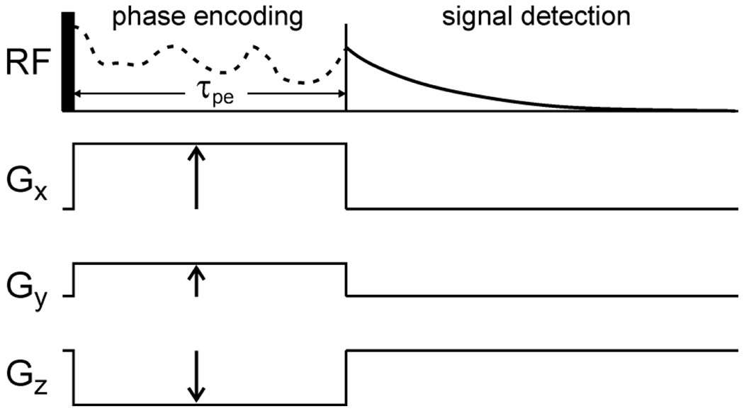
Simple MRI pulse sequence in which transverse nuclear spin magnetization, created by a single RF pulse, precesses in the presence of variable magnetic field gradients , , and during a constant phase encoding period , after which the NMR signals are detected. Each set of gradient amplitudes results in a complex signal that is proportional to the spatial Fourier component of the image at wave vector .
In order to develop an appreciation for the experimental feasibility of various gradient strengths, consider the magnetic field around an infinitely long, straight wire that carries a current I and lies in the xy plane, parallel to the x axis at a distance d from the origin. At points in the xy plane, the field is in the z direction with magnitude , where is the vacuum permeability (very close to in SI units). If I = 10.0 A, and d = 1.00 mm, . Now consider two such wires at displacements +d and −d from the origin, carrying the same current in the same direction so that their fields cancel along the x axis (i.e., when ). The z component of the total field is ; its gradient in the xy plane is . If I = 10.0 A and d = 1.00 mm, . From this example, it appears that gradients on the order of 10 T/m ( for 1H NMR signals) are readily achievable over sample dimensions less than 1 mm, using somewhat higher currents and/or multiple wires. Gradients on the order of 100 T/m are more challenging.
NMR signal decay during in Fig. 1 has the effect of reducing all k-space signal points by a factor of , where is the transverse spin relaxation time. The SNR of the image is thereby reduced, but the resolution is not affected directly. However, the total measurement time required to obtain a given SNR value increases by a factor of , which is a factor of 10 if . With pure phase encoding of the k-space data, as in the simple pulse sequence considered here, there is a clear trade-off between resolution and SNR when signal decay during is significant and when an upper limit on the total measurement time exists. (This is an important consideration in the low-temperature MRI experiments described below.)
In experiments above 0° C, translational diffusion by the molecules whose NMR signals give rise to the MR image is an important limiting factor for spatial resolution [25, 26]. Qualitatively, one expects translational diffusion to be a problem when the root-mean-squared (rms) distance traveled during , given by , is comparable to , where D is the translational diffusion constant. The condition that implies that the spatial resolution cannot be better than , as a rough estimate. With (appropriate for liquid water at 20° C) and G = 10 T/m, the lower limit on resolution obtained from this estimate is approximately .
For a more quantitative treatment of the effects of translational diffusion on a 1D image, consider the signal contribution from molecules that start at x = 0, then execute N random jumps by with time steps . This signal contribution, averaged over all combinations of random jump directions, can be expressed as
| (6) |
The small phase step in Eq. (6) represents the spin precession angle in one time step due to a displacement when the gradient is . The second line of Eq. (6) follows from the fact that jump directions in different time steps are uncorrelated, and for all j. The phase step can be expressed as , where is the 1D diffusion constant. Then Eq. (6) becomes
| (7) |
The derivative of with respect to k is
| (8) |
Only the first term in a Taylor series expansion of each sine function is retained in the second line of Eq. (8), as it can be shown that contributions from subsequent terms vanish as . It is also true that . Eq. (8) then becomes , which implies with . Thus, translational diffusion causes a Gaussian decay of signals in k-space, with decay constant .
In a 3D image, the signal decay from translational diffusion becomes , but with because the diffusion constant (defined so that the rms distance traveled in time t is ) becomes three times larger if the random jump distance is in all three dimensions. Using this expression, the broadening of spatial features in a 3D image due to translational diffusion can be evaluated from a point-spread function , which is the apparent shape in the image of an object that had nuclear spin polarization only at at the beginning of the phase encoding period:
| (9) |
Spatial features are broadened by convolution with the Gaussian point-spread function in Eq. (9), for which the full width at half maximum (FWHM) is . With and , the FWHM is . A factor of two reduction in the FWHM requires a factor of four reduction in , which in turn requires a factor of four increase in maximum gradient strengths. The condition that the FWHM of the point-spread function be less than the desired spatial resolution implies that , which means that maximum gradients must be greater than 116 T/m for 1H MRI with if . On the other hand, maximum gradients less than 10 T/m are sufficient to avoid effects of translational diffusion in images with [15, 16].
Note that Eq. (9) assumes free diffusion over distances greater than the FWHM of the point-spread function. Effects of restricted diffusion have been analyzed in several publications [27–29].
4. Abragam’s estimate of signal-to-noise in inductively detected NMR
As discussed above, achievable gradient strengths are not a fundamental limitation on spatial resolution in MRI at the level, provided the sample dimensions are small. Translational diffusion can be a limitation when diffusion constants are similar to that of pure water at room temperature. This limitation does not apply to the low-temperature MRI experiments described below. Instrumental stability can be a limitation, especially if the large current pulses required to produce magnetic field gradients cause the gradient coils to move micron-scale distances relative to the sample. The force on a 5 mm long wire that carries a 10 A current perpendicular to a 10 T field is 0.5 N, equal to the gravitational force on a 51 g mass on the Earth’s surface. This is not a tremendous force, but current pulses could excite vibrations that degrade the image resolution. In practice, the success of experimental demonstrations by several groups indicates that equipment with sufficient rigidity to avoid this problem can be constructed.
The remaining limitation, as has been discussed in previous work on micron-scale MRI [5, 11, 30], is the inherent SNR of NMR. An estimate of the SNR of time-domain NMR signals in a single scan appears in chapter III of Anatole Abragam’s book on “Principles of Nuclear Magnetism” [31]. Abragam’s estimate can be written in SI units as:
| (10) |
where and are the NMR frequency and receiver bandwidth, is the Boltzmann constant, and is the applied magnetic field. Signals are assumed to be detected by an ideal solenoid with volume V, inductance L, and resistance R. The quality factor Q of the solenoid equals . The filling factor equals the ratio of the sample volume to the solenoid volume. The nuclear magnetic susceptibility is in SI units, where S is the spin quantum number of the observed nuclei, is Planck’s constant divided by , and is the number of nuclear spins per unit volume.
Eq. (10) is the ratio of the amplitude of the signal voltage (more precisely, half of the peak-to-peak value of the oscillating electromotive force) induced in the solenoid by precessing transverse nuclear magnetization (equal to in SI units when a pulse is applied to spins whose polarization has equilibrated with the field at temperature T) to the rms Johnson noise voltage within a frequency range , arising from random thermally excited currents in the solenoid [32]. Precessing magnetization produces an oscillating magnetic flux in the solenoid, which can be written as if the sample fills the solenoid , where n is the number of turns and A is the cross-sectional area of the solenoid. For an ideal solenoid, . According to Faraday’s law of inductance, the signal is the (negative) rate of change of magnetic flux in the solenoid, which is then . The signal amplitude is if the sample does not completely fill the solenoid. The mean squared Johnson noise voltage per unit frequency interval [33] is . The rms noise within is then .
For the case of 1H NMR at 400 MHz with Q = 100, expressing the density of nuclei as a molar concentration c, Eq. (10) becomes
| (11) |
with V in milliliters, in Hz, and T in degrees Kelvin.
Eqs. (10) and (11) pertain to time-domain signals (i.e., free-induction decay signals) after a pulse. If the signals decay exponentially with transverse relaxation time , it can be shown that the frequency-domain SNR, defined as the NMR peak height divided by the rms noise in the spectrum with optimal apodization, is given by the same expressions, but with replaced by the NMR linewidth and with an additional factor of in the denominator. The frequency-domain SNR that follows from Abragam’s treatment is then
| (12) |
If , Eq. (12) predicts that a solution with and 1 Hz NMR linewidths in a solenoid (8 mm length, 4 mm diameter) with Q = 100 should give strong signals at room temperature in a single scan if . However, if the sample volume is only 27 femtoliters, corresponding to one volume element (one voxel) in an image with , then Eq. (12) yields even if c = 110 M, as in pure water. About 107 scans would be required to reach . This is because when a solenoid with volume is used to acquire data for an image with isotropic resolution, treating as the ratio of the voxel volume to the coil volume.
In principle, the use of solenoidal coils with sub-millimeter dimensions (i.e., microcoils) should largely solve the SNR problem. According to the analysis above, for a fixed voxel volume, SNR in an image should scale as . Eq. (12) predicts that a solenoid with volume (1.0 mm length, 0.36 mm diameter, or ) would allow from a volume of water at room temperature with only 104 scans. However, as discussed in more detail below, the SNR values in real micron-scale MRI measurements are less than the values predicted by Eq. (12) by large factors.
5. Signal-to-noise in real experiments
To be specific, Ciobanu et al. [15] achieved in 1H MR imaging of water at room temperature with voxels, , Hz, , and 204880 scans, whereas Eq. (12) yields in a single scan ( in 204880 scans). Weiger et al. [16] achieved with voxels, a planar microcoil with an effective volume (estimated from their images), , and 2.1 × 10⁶ scans, whereas Eq. (12) yields in a single scan ( in 2.1 × 10⁶ scans), assuming Hz and multiplying by (18.8/9.4)3/2 = 2.83 to account for the larger value of . In experiments by Moore and Tycko [21], was achieved for water at room temperature with voxels, , Hz, and 2.1 × 10⁶ scans, whereas Eq. (12) yields in a single scan ( in 2.1 × 10⁶ scans). Thus, in three independent efforts at micron-scale 1H MRI with microcoils at room temperature, the actual SNR values were about two orders of magnitude (factors of 50-150) lower than predicted by Eq. (12).
What accounts for the discrepancies from the SNR predicted by Eq. (12)? relaxation during phase encoding periods in the MRI pulse sequences, separate acquisition of real and imaginary parts of in some pulse sequences, incomplete recovery of nuclear spin magnetization between scans due to short recycle delays, signal losses in cables and transmit/receive circuitry, and non-zero receiver noise figures could reduce the SNR by a factor of 2-6, roughly speaking. A factor of 10 or more is still missing.
Is it possible that signals are reduced significantly by the fact that microcoils are not ideal solenoids, i.e., that the turn spacings are not negligible compared to the microcoil diameters and the diameters are not negligible compared to the microcoil lengths? For a general coil structure, the signal cannot be calculated from Faraday’s law of induction because the magnetic flux is not well defined. Instead, one can use the corresponding Maxwell equation, i.e., in SI units. Considering a vector potential defined by , one obtains , where is an arbitrary potential function that can be attributed to electric fields from static charges and ignored. The signal, or electromotive force, is then , where the integral is over the path of the coil windings. This is the generalization of Faraday’s law of induction for an arbitrary coil structure constructed from thin wire. If the time-varying magnetic field is produced by precessing magnetic moments with density within a total volume V, then is the time-dependent vector potential at position . The total electromotive force in the coil is then . The contribution to the signal per volume from precessing magnetic moments at is
| (13) |
On the other hand, if current I is flowing in the coil, the magnetic field at position , calculated according to the Biot-Savart law in SI units, is . Hence
| (14) |
Comparing Eqs. (13) and (14), it is clear that the signal amplitude produced by precessing magnetic moments at the origin is proportional to the magnitude of the magnetic field in the xy plane at the origin produced by unit current (assuming that the same coil is used in both cases). The same result would be obtained for a magnetic moment at any position , since the origin of the coordinate system can be defined arbitrarily. Thus, one arrives at the “principal of reciprocity” that is frequently invoked in treatments of NMR sensitivity and coil designs [11, 34–37]:
| (15) |
If the sample is localized to a small volume within which and are nearly constant, the SNR expression in Eq. (10) then generalizes to
| (16) |
with the nuclear magnetization being . With V in milliliters, in Hz, T in degrees Kelvin, proton concentration c in moles per liter, R in ohms, and in Tesla per amp, Eq. (16) yields for 1H NMR at 400 MHz. The corresponding frequency-domain expression is .
Comparison of Eqs. (10) and (16) yields . Eq. (10) can be derived from Eq. (16) by using properties of an ideal solenoid, i.e., and .
Using Eq. (14), one can calculate exactly the value of for a helical solenoid that is centered at the origin and aligned with the x axis. If this solenoid comprises n turns and has length and diameter , the result is
| (17) |
Compared with the result for an ideal solenoid, is smaller by a factor of , which is 0.970 if . is non-zero for the helical solenoid, but is much smaller than if . Thus, according to Eq. (15), the predicted signal from a voxel in the center of a helical solenoid with realistic length, diameter, and turn spacing is not much smaller than the predicted signal from a voxel in the center of an ideal solenoid with the same number of turns per unit length.
By assuming an ideal solenoid, Abragam obtained a simple relation between signal and inductance that leads to Eq. (10) when . The inductance of a helical solenoid with realistic dimensions is less than that of an ideal solenoid by a factor on the order of 0.5, although the NMR signal from nuclear spins in the center of the solenoid is nearly unchanged. If the inductance of a helical solenoid is expressed as with , then . Thus, for given values of Q and V, Eq. (10) apparently underestimates the SNR relative to what is expected from a helical solenoid with realistic dimensions.
Is the noise from realistic microcoils much larger than assumed in Eq. (12), i.e., is ? A thorough treatment of the dependence of R (and hence Q) on microcoil dimensions has been given by Peck et al. [36]. Assuming that all dimensions of the coil (including wire thickness) scale together, they show that in the low-frequency or small-coil regime, where the wire thickness is less than the “skin depth”, i.e., the characteristic distance from the wire surface within which RF currents flow. In the opposite regime, R is independent of V. When combined with Eq. (17), which says that the signal arising from material in a fixed voxel volume scales as or , the dependence of R on V implies that the SNR from a fixed voxel volume should scale as in the small-coil regime and as in the opposite regime. Peck et al. present experimental data from 1H NMR measurements at 4.7 T with microcoil diameters in the 50-2000 range that support these predicted dependences, with a cross-over to the small-coil regime below . In contrast, Eq. (12) predicts that SNR scales as if Q is constant (i.e., independent of V).
Peck et al. state that their microcoils had Q values in the 10-70 range [36], which implies that their SNR values should not be more than three times lower than values predicted by Eq. (11). They report time-domain SNR values approximately equal to 14 in a single scan with Hz for microcoils with volumes of approximately and water samples with , whereas Eq. (11) predicts after accounting for the lower value of in the experiments of Peck et al.
The considerations and results described above indicate that a major part of the discrepancy between experimentally observed SNR values and values predicted from theoretical analyses of single coils is not attributable to non-idealities of the coils themselves. Instead, it appears that circuit elements other than the microcoil make dominant contributions. These circuit elements include leads to the microcoil, capacitors used for tuning and impedance matching, and connections to ground. Inevitably, these circuit elements have their own resistances and hence contribute Johnson noise. RF magnetic fields associated with leads and connections to ground also make smaller than the value calculated from the microcoil volume alone. However, these contributions from other circuit elements should only be important when the elements in question are included in the resonant part of the NMR probe circuit, i.e., the part of the circuit where currents and voltages are amplified by the Q factor. For example, in the case of an ideal circuit comprising an inductor L (the sample coil), a tuning capacitor in parallel with the inductor, and a matching capacitor in series with the combination, resistances in L, , their connections to one another, and their connections to ground contribute to Q and to the expected SNR. Extra resistances in , connections between and , and connections between and the cable through which signals go to the receiver of the spectrometer have little effect on the SNR, provided that Q is not small and the extra resistances are not very large.
It should be noted that Seeber et al. [38] also reported extensive measurements of SNR values for 1H NMR of water at 9.0 T, obtained with microcoil volumes ranging from to . Their experimental values of SNR per volume of water follow an approximate dependence, as predicted by Eq. (10) with a fixed value of Q, although their measured Q values varied from 5 to 30. They report a value of the SNR per cubic micron of water approximately equal to 0.15 in one scan at room temperature, with Hz, using a microcoil with and . According to Eqs. (10-12), for these parameters. The experiments of Seeber et al. used a very compact probe circuit, with minimal lead lengths and without an impedance matching network, apparently contributing to the relatively good agreement between measured and predicted SNR values. On the other hand, the SNR in subsequent MRI experiments by the same research group did not match simple predictions [15], as discussed above.
In related work, Grisi et al. [37] described the design and performance of a single-chip NMR transceiver, including an integrated planar microcoil with diameter. Experimental results with this device included a frequency-domain SNR value of approximately 250 in the 300 MHz 1H NMR spectrum of ammonium hexafluorophosphate, for which kHz, obtained with 5000 scans. (This SNR value was determined by digitizing the time-domain data shown in the publication of Grisi et al. [37], applying optimal apodization, Fourier transforming the apodized data, and evaluating the ratio of the peak height to the rms noise in the processed data.) Assuming an effective coil volume of approximately , and a 1H density of 53 M, and correcting for the smaller value of B0, Eq. (12) predicts . However, the assumption in Eq. (12) that Q = 100 is unjustified in this case. Grisi et al. report and for their planar microcoil, making the predicted value of at 300 MHz and 300 K equal to 220 with 5000 scans, , and c = 53 M.
In other related work, Minard and Wind reported a frequency-domain SNR of 4.4 ± 0.9 for methyl protons in the 500 MHz 1H NMR spectrum of 33 mM choline chloride, obtained from a voxel within a microcoil volume of (i.e., . The apparatus used by Minard and Wind was designed to minimize losses and inductance outside the microcoil itself. A chemical shift imaging (CSI) technique was used, with a total of 4096 scans and . Taking into account the nine methyl protons per choline molecule and the larger value of , Eq. (12) predicts . As discussed by Minard and Wind, the predicted SNR value should be corrected to account for the Q of their microcoil and for signal losses from spin relaxation and translational diffusion during the CSI pulse sequence, thereby reducing the predicted value of by a net factor of 0.38.
Results discussed above therefore indicate that experimental SNR values close to theoretical values based on properties of the microcoil alone can be achieved with circuitry that minimizes losses in other circuit elements. However, SNR values close to theoretical values have not yet been achieved in MRI experiments with .
6. Micron-scale MRI at low temperatures
6.1. MRI pulse sequence including Lee-Goldburg decoupling and pulsed spin-lock detection
The foregoing discussion, together with experimental results from several groups [15, 16, 21], demonstrates that the practical resolution limit for inductively detected 1H MRI at room temperature is approximately , even with microcoils, long measurement times, and samples that have 100% contrast. This limit is set primarily by SNR considerations, implying that large enhancements in SNR are required to achieve higher resolution. One way to enhance the SNR is to reduce the temperature T of the sample and probe circuitry. In principle, a reduction of T from 300 K to 10 K should increase the SNR by a factor of 164, if nothing else changes in Eq. (12), and thereby improve the accessible isotropic spatial resolution by a factor of (164)1/3 = 5.5. At low temperatures, large additional SNR enhancements can be obtained with dynamic nuclear polarization (DNP) [22, 39–42]. These simple ideas encouraged members of the author’s laboratory to pursue low-temperature MRI experiments, first without DNP [20] and later with DNP [19, 43].
At low temperatures, the sample is a solid, rather than a liquid or liquid-like in its NMR properties. This immediately changes two important parameters. First, 1H nuclear spin-lattice relaxation times at low temperatures can be longer than 100 s in a diamagnetic solid that lacks large-amplitude internal molecular motions such as methyl group rotations, thereby reducing the SNR obtainable in a given measurement time by a factor greater than 10. In experiments on frozen solutions without DNP, this problem can be overcome by the addition of paramagnetic ions such as to the solution [44].
Second, 1H NMR lines are strongly broadened by static nuclear magnetic dipole-dipole couplings in a solid. 1H NMR linewidths in a fully protonated solid are typically around 50 kHz, which reduces the SNR in a simple spectroscopic NMR measurement by a factor of about 200-300 relative to the SNR from a liquid, according to Eq. (10). In an MRI measurement, large 1, because signals are reduced by a factor of or , with being approximately the inverse of the linewidth. MRI techniques for solids have been designed to overcome these effects by removing or refocusing the impact of dipole-dipole couplings on linewidths in a variety of ways [45–59].
Low-temperature MRI experiments in the author’s laboratory have used pulse sequences of the type shown in Fig. 2a. In the signal detection period, pulsed spin-locking (PSL) with digitization of 1H NMR signals in intervals between RF pulses is used to extend the signals well beyond the natural decay time [60–64]. In measurements on frozen glycerol/water solutions, for which the value determined by 1H-1H dipole-dipole couplings in the absence of PSL is about (and the decay is nearly Gaussian in form), signal decay times can be extended to 50 ms or more by PSL [20, 22, 65]. The effectiveness of PSL is increased by the use of microcoils, which easily allow the individual PSL pulses to be or less with flip angles of 45°-90°. PSL largely overcomes the first deleterious effect of static dipole-dipole couplings on the SNR.
Figure 2:
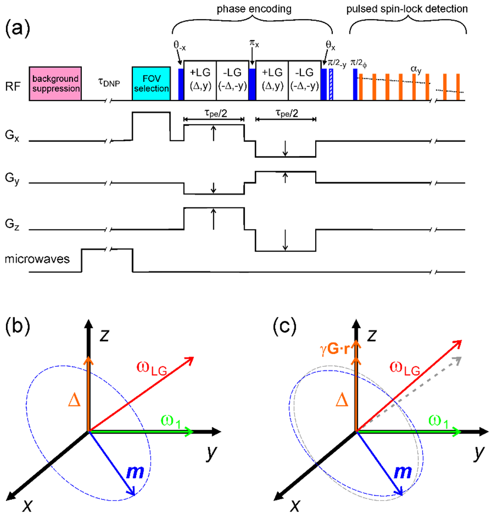
(a) Pulse sequence for DNP-enhanced 1H MRI at low temperatures. A train of RF pulses is first applied to eliminate nuclear spin polarization and suppress NMR signals from 1H in background material. Microwaves are applied during to partially saturate the electron spin polarization of paramagnetic dopants, resulting in enhanced 1H nuclear spin polarization within the sample. (In experiments without DNP, microwaves are not applied, and 1H nuclear spin polarization builds up towards its thermal equilibrium value during .) If desired, RF pulses can then be applied in the presence of a strong magnetic field gradient to select the polarization within a restricted FOV, using a variety of approaches [19–21, 43]. During the constant phase encoding period, 1H-1H dipole-dipole couplings are attenuated by LG irradiation and variable gradients are applied in x, y, and z directions. The gradients change sign after a pulse so that precession due to the gradients is not refocused. After the phase encoding period, 1H NMR signals are detected under PSL, with signals being digitized in windows between short spin-locking pulses with flip angles . Pulse phase alternates between x and −x and signals are alternately added and subtracted to cancel ring-down artifacts from the PSL pulses. (b) In +LG periods, nuclear spin magnetization m, prepared by the pulse, precesses about an effective field with amplitude , which is the resultant of y and z components equal to and Δ in the usual rotating frame. In -LG periods, these components change sign to cancel effects of RF inhomogeneity. At the end of the phase encoding period, the component of m perpendicular to the plane or parallel to x (i.e., real or imaginary component) is stored along z (and subsequently detected in the PSL period) by application of the pulse or the and pulses. (c) When gradient pulses are applied, the z component becomes , causing the magnitude of to change and resulting in a net precession of m that carries the image information.
In the phase encoding period, Lee-Goldburg (LG) irradiation [50, 66–69] is applied to average out dipole-dipole couplings without removing NMR frequency offsets created by magnetic field gradient pulses. LG irradiation consists of the application of an RF field with amplitude and resonance offset (in the absence of gradients) , creating an effective field in the rotating frame that has amplitude and makes an angle with the z axis, as shown in Fig. 2b. Provided that is very large compared to the dipole-dipole coupling strengths, dipole-dipole couplings are ideally removed when , which makes , the “magic angle”. Resonance offsets created by gradient pulses are scaled by a factor of , which is the projection of a unit vector along z onto the effective RF field direction in the rotating frame. In practice, LG irradiation attenuates 1H-1H dipole-dipole couplings by an approximate factor of 100 in experiments on frozen glycerol/water solutions when kHz [20]. This allows values of in the 0.6-0.8 ms range to be used in low-temperature MRI experiments without large signal losses. Thus, LG irradiation can largely overcome the second deleterious effect of static dipole-dipole couplings described above.
In the presence of gradient pulses, the resonance offsets become and becomes , as shown in Fig. 2c. For a fully protonated solid, LG irradiation is an acceptable method for attenuating dipole-dipole couplings as long as (i.e., )[20, 21]. This condition implies that . With and maximum gradients on the order of ( for nuclei), the projection of onto should then be between and to avoid degradation of the spatial resolution. Thus, the sensitivity of LG decoupling to gradient strengths can limit the FOV within which high spatial resolution is obtained. Reduction of 1H-1H dipole-dipole coupling strengths by partial deuteration, as in DNP-enhanced experiments described below, increases the accessible FOV. If the permissible value of is inversely proportional to the fraction of hydrogen nuclei that are 1H rather than 2H, then the accessible FOV is expected to be proportional to .
Alternatively, the accessible FOV of LG-based imaging methods may be increased in principle by including RF gradients in such a way that becomes approximately independent of r [50–52]. However, for micron-scale MRI of a solid sample, this approach would require elaborate combinations of microcoils.
In the pulse sequence in Fig. 2a, nuclear spin magnetization is prepared initially perpendicular to the effective field in the rotating frame by a pulse, with flip angle . The RF phase switches between +y and −y in +LG and −LG periods, respectively. The RF carrier frequency also switches, such that the resonance offset is either or . With this phase and frequency switching, spin precession about the effective field cancels between the +LG and −LG periods when , regardless of the value of . NMR signals are then insensitive to RF inhomogeneity. A pulse in the middle of the LG period refocuses precession due to constant resonance offsets that may arise from chemical shifts or static magnetic field inhomogeneity. Gradient pulses with opposite signs are applied before and after the pulse, so that precession due to (which contains the desired image information) is not refocused. Real or imaginary parts of complex signals are measured in separate PSL signals by applying either a pulse at the end of the LG decoupling period (i.e., the phase encoding period) or a pulse followed by a pulse.
Pulse imperfections can produce magnetization components that are parallel, rather than perpendicular, to the effective fields during the LG decoupling period. Because these components do not precess in the rotating frame, they can create strong artifacts in the images at (i.e., in the apparent center point of the gradients). The dependence of the effective field direction on when strong gradient pulses are applied provides one potential source of parallel magnetization components and image artifacts, for example because the pulse cannot prepare all of the magnetization perpendicular to the effective field if the effective field direction varies. This problem can be minimized by applying the , and pulses in the absence of gradients and switching the gradients on and off adiabatically, so that precessing magnetization remains perpendicular to the effective field even as the effective field direction changes [19].
Suppression of background 1H NMR signals is essential in low-temperature 1H MRI experiments, since signals from the region of interest within the microcoil are small relative to background signals that would otherwise arise from glue, grease, wire insulation, or other sources. One approach to background signal suppression, which relies on the difference in RF field amplitudes within and outside the region of interest, is to apply a train of pulses separated by delays for dephasing of transverse magnetization, together with a narrowband composite pulse that is applied on alternate scans [21]. To further restrict the final signals to a smaller volume within the microcoil, the train of pulses can be applied in the presence of a strong field gradient parallel to the long axis of the microcoil (i.e., the x axis), with RF amplitudes adjusted to select signals within a single interval of x values [19]. Restriction of the final signals to a smaller volume, i.e., a smaller FOV, can reduce the total time required to obtain a complete set of high-resolution image data.
Reduction of the FOV (i.e., slice selection) in the presence of strong 1H-1H dipole-dipole couplings can also be carried out by aligning the 1H magnetization with a strong LG field, applying a strong field gradient along x, and modulating the RF phase (at frequency ) in a precisely controlled manner that results in magnetization inversion only within a limited range of x values. This approach allows the position, size, and shape of the selected slice to be varied by appropriate adjustments to the frequency, amplitude, and shape of the RF phase modulation [43].
6.2. Experimental apparatus and implementation
The compact MRI apparatus depicted in Fig. 3 was used to demonstrate micron-scale MRI at low temperatures, based on pulse sequences of the type shown in Fig. 2a. Full details of this apparatus, with minor variations, are given in several papers [19–21]. The heart of the apparatus is a stack of rectangular sapphire plates (31.5 mm × 6.1 mm × 1.5 mm) that are mounted on the temperature-controlled copper block of a variable-temperature, helium-cooled cryostat. The interior of the cryostat is pumped to high vacuum during operation. The microcoil and the x and y gradient coils are glued into slots in the surfaces of the inner sapphire plates. A pair of z gradient coils are glued to the surfaces of the outer sapphire plates. Holes in the plates provide a path for microwave irradiation and allow the plates to be attached to the copper block with brass screws.
Figure 3:
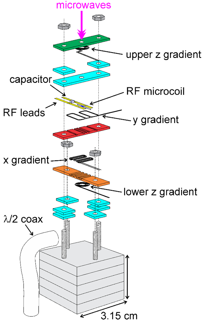
Schematic exploded view of the apparatus used in low-temperature MRI experiments. The RF microcoil, containing the sample, and coils for x and y gradients are glued within slots in red and orange plates (31.5 mm × 6.1 mm × 1.5 mm plate dimensions). Coils for the z gradient are glued to the surfaces of green and orange plates. Additional cyan plates serve as spacers. Holes in the plates provide a path for microwave irradiation. A stack of thicker plates (grey, 31.5 mm × 31.5 mm × 5.1 mm) connect the assembly to a temperature-controlled copper block in the variable-temperature cryostat. All plates are made of sapphire for high thermal conductivity. A ceramic chip capacitor increases the effective inductance of the microcoil, which is connected to other RF circuit elements (not shown) by a rigid coaxial cable. (Adapted from Chen and Tycko, J. Magn. Reson. 2018 [20].)
The high thermal conductivity of sapphire ensures that the temperature of the sample within the microcoil is nearly equal to the temperature of the copper block, which can be varied from 4.2 K (or lower if a vacuum pump is attached to the helium exhaust port of the cryostat) to 300 K. Thermal anchoring of gradient coils to the sapphire plates also allows 100 A current pulses with durations of several milliseconds to be applied without damage, even though the diameter of the gradient coil wires is only 0.26 mm. Gradient strengths in the x, y, and z directions at low temperatures [19] are approximately 0.35 T/A-m, 0.39 T/A-m, and 0.44 T/A-m, respectively, and are uniform to within 5% over a volume of approximately [21].
In published experiments, microcoils were wound around and glued to fused silica capillary tubes with 100-150 outer diameters, using 8 turns of copper wire with diameter. 1H RF amplitudes of 220-250 kHz were achieved with roughly 10 mW of RF power at 399.2 MHz. Microcoils and samples could be changed by disassembling and reassembling the stack of sapphire plates. For experiments with DNP, microwave powers of 30-50 mW near 263 GHz were supplied by tunable solid-state sources and transmitted to the sample by a combination of quasi-optical components and a corrugated waveguide outside the cryostat and by a corrugated, tapered horn and tapered polytetrafluoroethylene piece within the cryostat [19].
Plots in Fig. 4 show some of the optimizations that are relevant to imaging experiments with pulse sequences of the type in Fig. 2a. In low-temperature experiments without DNP, DY3+ was added to glycerol/water solutions to reduce . [20] As shown in Fig. 4a, the dependence of on temperature indicates an optimum value near 30 K. Fig. 4b shows that the total time-domain 1H NMR signal area under PSL is not determined simply by the average spin-locking field strength, but instead depends strongly on the flip angle and spacing between PSL pulses (Fig. 4b). Dependences of the signal area on the RF carrier frequency and RF amplitude during LG irradiation and on the value of were also characterized, as shown in Figs. 4c-4f.
Figure 4:
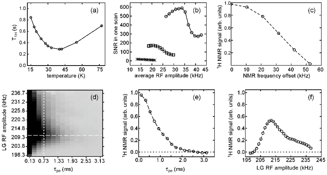
Optimization of pulse sequence parameters for low-temperature 1H MRI in a 9.39 T field. (a) Dependence of the 1H spin-lattice relaxation time on temperature for a frozen glycerol/water solution containing 4 mM Dy3+. The SNR in a fixed total experiment time is maximized at . (b) Dependence of the total area of the time-domain 1H NMR signal under PSL on the average RF amplitude, using 1.0 PSL pulses without a variable amplitude and inter-pulse delays of 4.2 (circles), 6.2 (squares), and 8.2 (crosses). The signal is maximized with pulse amplitudes near 175 kHz and flip angles . (c) Dependence of the 1H NMR signal on NMR frequency offset during LG irradiation, using and , . (d) Dependence of the 1H NMR signal on and the RF amplitude during LG irradiation, with darker shades representing stronger signals. (e) Horizontal slice from panel d, showing the dependence on . (f) Vertical slice from panel e, showing the dependence on the RF amplitude. (Adapted from Chen and Tycko, J. Magn. Reson. 2018 [20].)
6.3. Results without DNP: 2.8 micron resolution at 28 K
Initial experiments to test the apparatus described above were performed at room temperature, using both liquid ( diameter polystyrene beads in Cu2+-doped water) and solid (NH4Cl particles) samples [21]. In liquid state MRI experiments, 5.0 isotropic resolution was achieved over a FOV, with in 150 h of data acquisition (2.1 × 10⁶ scans). In solid state MRI experiments, 8.0 isotropic resolution was achieved over a FOV, with in 64 h of data acquisition (4.6 × 10⁵ scans). In terms of spatial resolution, this result was considerably better than results from any previously reported solid state MRI experiments [45–48, 50–52, 54, 57, 59, 70, 71], other than experiments based on force-detected NMR signals [72–78].
Experiments were then performed at 28 K without DNP [20], yielding a 1H MR image of glass beads in Dy3+-doped glycerol/water with 2.8 isotropic resolution, a FOV, and a total data acquisition time of 52 h (3.8 × 10⁵ scans; Fig. 5). These experiments demonstrated that images of solid samples at low temperatures can have slightly higher resolution than the best previously reported images of liquids at room temperature, despite the complications introduced by strong 1H-1H dipole-dipole couplings at low temperatures. Even without signal enhancements from DNP, the SNR advantages of low temperatures can overcome the disadvantages of dipolar-broadened NMR lines when pulse sequences of the type shown in Fig. 2a are used.
Figure 5:
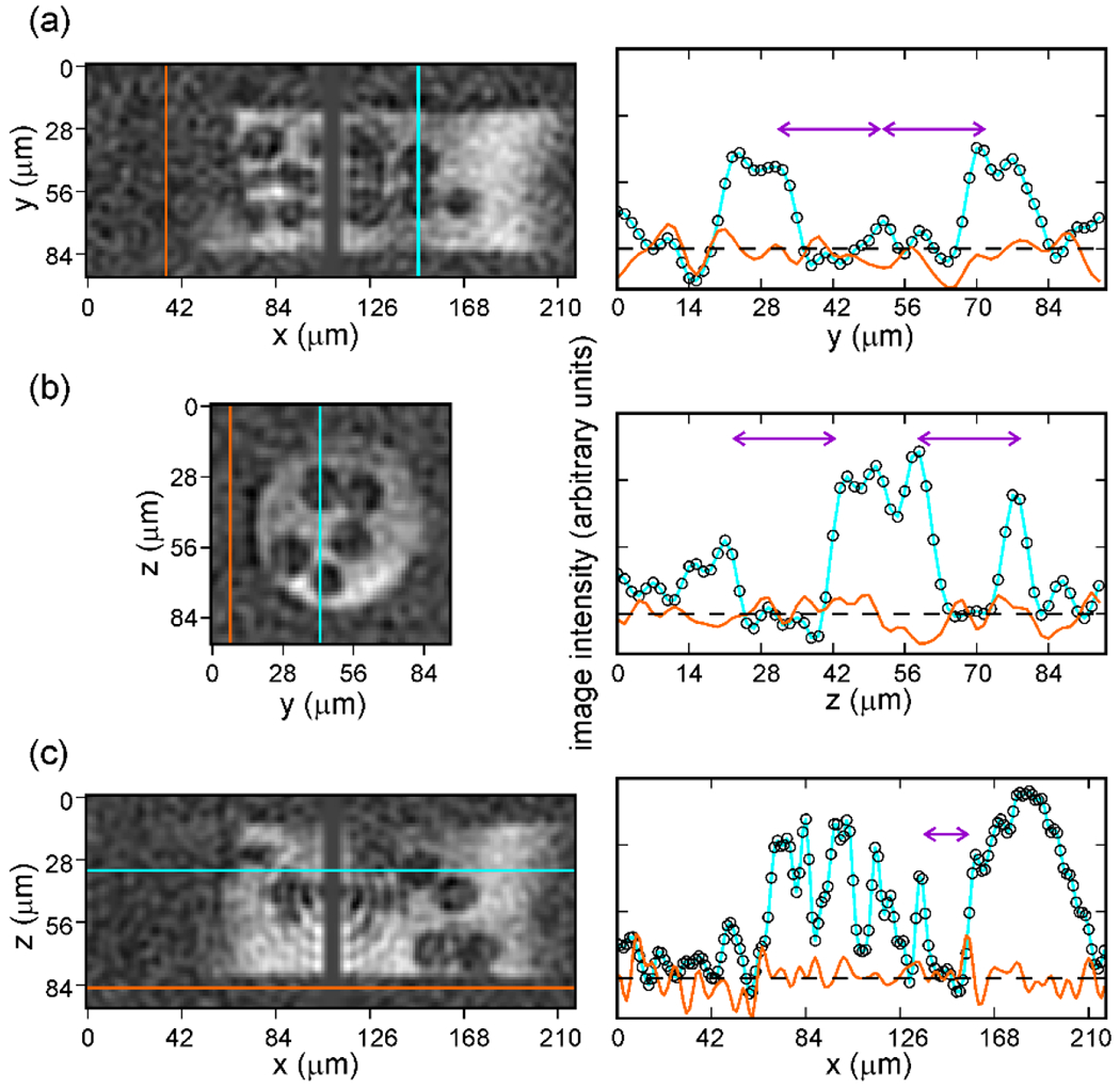
1H MR image of glass beads in Dy3+-doped glycerol/water, contained in a capillary tube with 75 inner diameter, recorded at 28 K with . 2D slices in the xy, yz, and xz planes (panels a, b, and c, respectively) are shown on the left. Color-coded 1D slices along the cyan and orange lines are shown on the right. Double-headed purple arrows indicate 20 distances in each 1D slice, corresponding to the diameter of one glass bead. (Adapted from Chen and Tycko, J. Magn. Reson. 2018 [20].)
6.4. Results with DNP: 1.7 micron isotropic resolution at 5 K
DNP based on the cross effect mechanism [79, 80] can produce enhancements of 1H nuclear spin polarizations, relative to thermal equilibrium polarizations, by factors on the order of 100 in measurements on frozen aqueous solutions that are doped with biradical [81–84] or triradical [42, 85–87] compounds based on nitroxide groups or similar moieties. Examples of signal enhancements from DNP and dependencies of sensitivity enhancements on temperature are shown in Figs. 6a-6c.
Figure 6:
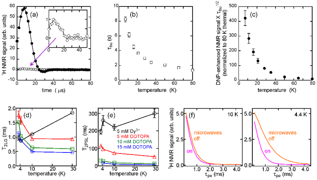
Properties of DNP-enhanced 1H NMR signals at low temperatures. (a) Solid echo signals from frozen glycerol/water containing 30 mM DOTOPA triradical. Signals were acquired at 11 K and 9.39 T with (filled circles) and without (open circles) irradiation from a 30 mW microwave source operating at 264.0 GHz. (b) Temperature-dependence of the build-up time for DNP-enhanced 1H nuclear spin polarization. (c) Temperature-dependence of the net DNP sensitivity enhancement relative to signals at 80 K without microwave irradiation. (d) Temperature-dependence of the dephasing time during LG irradiation with for signals obtained with a pulse sequence similar to that in Fig. 2a, without field gradient pulses and without microwave irradiation. Data are shown for glycerol/water samples with 97.5% deuteration, containing 5 mM Dy3+ (black circles), 5 mM DOTOPA (red triangles), 10 mM DOTOPA (green triangles), and 15 mM DOTOPA (blue pentagons). (e) Temperature-dependence of the dephasing time during pulsed spin locking for the same samples as in panel d. (f) Dependences of DNP-enhanced signals on at 10 K and 4.4 K, with (magenta) and without (orange) microwave irradiation during the phase encoding period of the pulse sequence. At 4.4 K, signal decay is slower without microwave irradiation because electron spins become strongly polarized in the absence of microwaves, thereby suppressing electron-electron spin flip-flop transitions that lead to dephasing of nuclear spin magnetization. (Adapted from Thurber et al., J. Magn. Reson. 2010 [42] and Chen and Tycko, J. Phys. Chem. B 2018 [65].)
If 2.8 isotropic resolution can be achieved at 28 K without DNP, a SNR enhancement of 100 should permit 0.6 resolution (provided that gradient strengths can also be increased appropriately). However, the introduction of paramagnetic DNP dopants at concentrations required for large polarization enhancements results in reductions in transverse nuclear spin relaxation times [22, 65, 88], thereby reducing SNR enhancements. In addition, the build-up times for DNP-enhanced 1H spin polarizations in fully protonated frozen solutions at temperatures below 30 K are on the order of 10 s or more with moderate dopant concentrations [19, 42, 65, 88], further reducing sensitivity gains from DNP.
Reductions in transverse nuclear spin relaxation times are attributable to the presence of local fields at the nuclei from the magnetic moments of nearby unpaired electron spins. These fields fluctuate when couplings among electron spins cause electron-electron flip-flop transitions, resulting in dephasing of transverse nuclear spin magnetization. The flip-flop transitions require that pairs of coupled electron spins be in opposite states, i.e., that one electron spin be in its | + > state and the other be in its | − > state. At sufficiently low temperatures and high magnetic fields, the electron spins are highly polarized at thermal equilibrium, i.e., nearly all electrons are in the | + > state. Flip-flop transitions should then become infrequent and transverse nuclear spin relaxation times should become longer.
Electron spins become highly polarized in a 9.39 T field at temperatures below 12.6 K, which is the temperature at which , with rad/s-T being the electron gyromagnetic ratio. Figs. 6d and 6e shows experimental measurements of transverse relaxation times and for 1H spins in triradical-doped water/glycerol solutions during the LG irradiation and PSL periods of a pulse sequence of the type shown in Fig. 2a. These measurements verify that the deleterious effects of electron-electron flip-flop transitions on the SNR (and hence the spatial resolution) of DNP-enhanced 1H MRI experiments can be reduced by performing the experiments at temperatures near that of liquid helium. At relatively low electron spin concentrations and high deuteration levels, for 1H spins in frozen glycerol/water increases to 1.7 ms near 4 K (Fig. 6d), allowing to be greater than 1 ms. increases to 100 ms (Fig. 6e), resulting in an effective 1H linewidth of roughly 3 Hz under PSL in the signal detection period of the imaging experiment. As shown in Fig. 6f, transverse relaxation times for 1H spins at very low temperatures are reduced when microwave irradiation is applied, consistent with the idea that the transverse relaxation times for nuclear spins depend on the population of electron spins in their higher-energy state. Therefore, it is advantageous to apply microwaves only in the period of Fig. 2a.
Experiments to demonstrate DNP-enhanced 1H MRI at 5 K were performed by Chen and coworkers [19] on samples consisting of 9.2 diameter silica beads in frozen solutions comprising 10% H2O, 30% D2O, and 60% perdeuterated glycerol by volume, with 12 mM of the triradical compound succinyl-DOTOPA [86], contained within a capillary tube with inner diameter. Signal enhancements from DNP were maximized by combining the outputs of two microwave sources with perpendicular planes of linear polarization, using a quasi-optical system, and optimizing their frequencies and frequency modulation amplitudes. Under optimized conditions, was 6.2 s at 5 K. Values of and were approximately 0.7 ms and 27 ms, respectively. The microcoil length was , with eight turns of diameter wire wrapped around the outer diameter of the capillary tube.
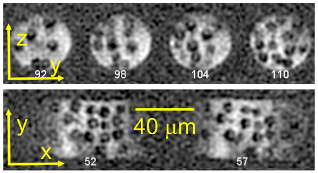
With these conditions, Chen and coworkers obtained an image with (achieved with and maximum gradient strengths of approximately 31 T/m, or 1.3 kHz/ for 1H NMR), a FOV, and SNR = 15.5, with a total measurement time of 80.6 h. A total of 32,102 complex k-space points were acquired, with spherical sampling of k-space (i.e., measurement of points with ), and four scans per complex point. The microwave irradiation time was set to 2.0 s. Examples of 2D planes from the 3D image are shown in Fig. 7.
Figure 7:
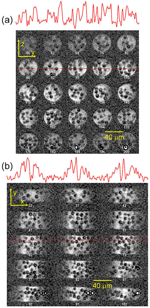
DNP-enhanced 1H MR image with , recorded at 5 K and 9.39 T. The sample is 9.2 diameter silica beads in 90% deuterated glycerol/water with 12 mM succinyl-DOTOPA triradical dopant, contained within a capillary tube with 40 inner diameter. (a) 2D slices in the yz plane, separated by 2.35 increments in z. (b) 2D slices in the xy plane, separated by 2.13 increments in z. 1D slices at the positions of dashed red lines are shown above each set of 2D slices. (Reproduced from Chen et al., Proc. Natl. Acad. Sci. USA 2022 [19].)
To verify that the true image resolution was 1.7 , Chen and coworkers made several comparisons between experimental and simulated images [19]. One such comparison is shown in Fig. 8a. Additionally, the silica beads in Fig. 7 appear as dark balls with bright spots in their centers. Simulations in Fig. 8b show that the bright central spots result from truncation of spherically-sampled k-space data, which produces oscillatory artifacts after zero-filling and Fourier transformation (i.e., the “truncation wiggles” that are familiar to NMR spectroscopists). A bright central spot occurs when oscillations that emanate from the spherical boundary between the dark bead and the bright solvent add constructively in the center of the bead. For beads with 9.2 diameter, bright spots occur only when .
Figure 8:
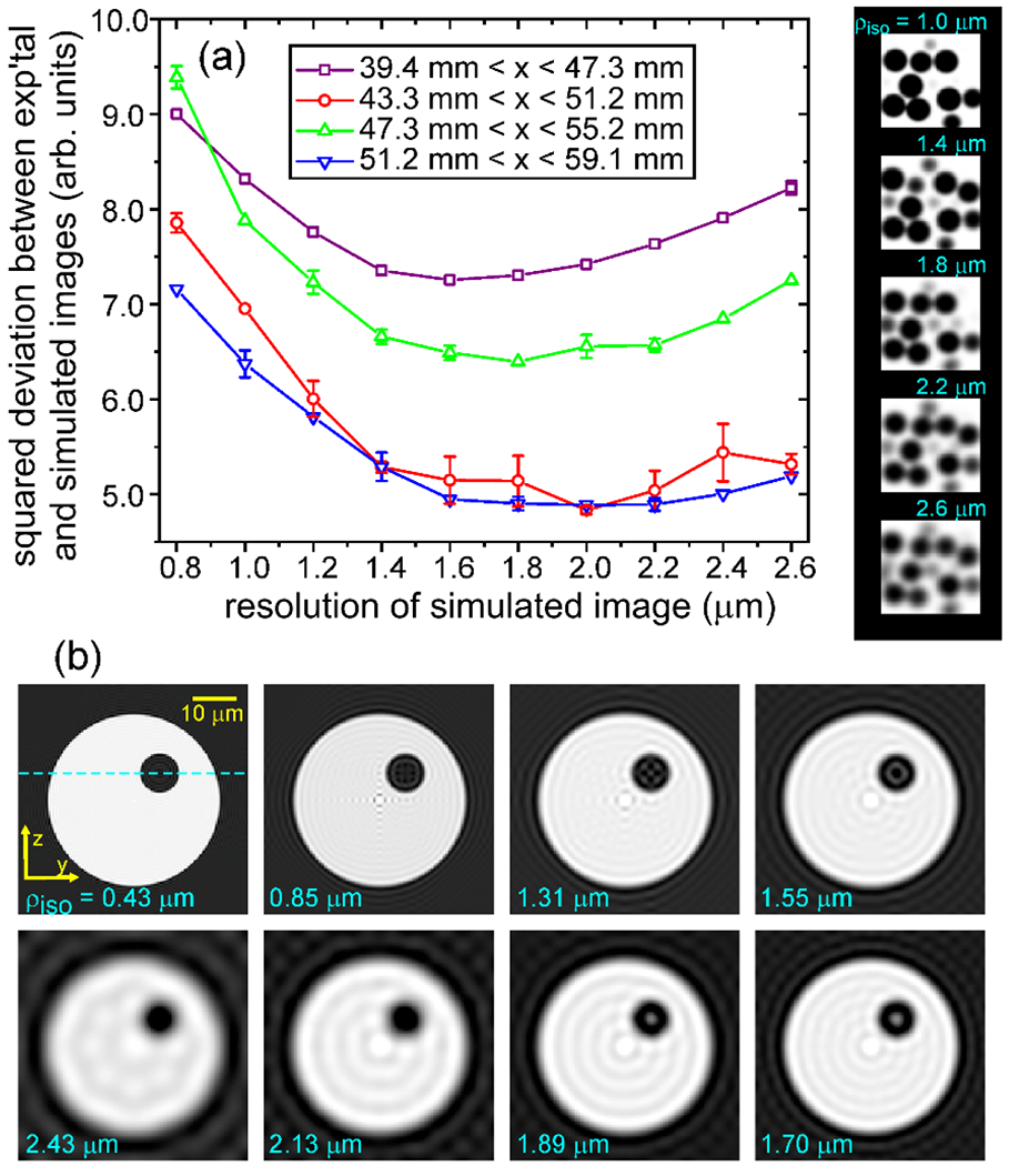
Verifications of 1.7 spatial resolution. (a) Total squared deviations between intensities in sections of the experimental image in Fig. 7 and corresponding sections of a simulated image of 9.2 diameter spheres, as a function of the resolution of the simulated image. Positions of spheres in the simulated image and overall intensity scales were adjusted to minimize the deviations. The resolution of the simulated image was varied by convolving with a Gaussian “blurring” function, as depicted to the right of the plot. Total squared deviations were minimized at resolutions near 1.7 in all image sections. (b) Cross-sections of simulated images of a single 9.2 diameter sphere in capillary tube with 40 inner diameter. In these simulations, images were generated by Fourier transformation of simulated k-space data sets with . Due to data truncation effects, a bright spot appears in the center of the sphere in simulations with . Similar bright spots are observed in the experimental image in Fig. 7.
7. Prospects for further improvements in resolution
In terms of voxel volume, results obtained by Chen and coworkers with DNP at 5 K represent an improvement by a factor of 5.5 relative to 1H MR images with the highest resolution obtained previously at room temperature [16]. Further developments in two areas may lead to images with .
First, improvements in hardware are likely to have a significant impact. In the NMR spectrometer used by Chen and coworkers, the transmit/receive network and the preamplifier of the receiver section operated at room temperature. The receiver noise figure was approximately 1.0 dB, corresponding to a noise temperature of approximately 80 K. If the RF circuitry within the cryostat is at 5 K, a receiver noise temperature of 80 K means that the SNR is reduced by a factor of 4.1 relative to the value that would be observed if the receiver noise temperature was well below 5 K. Thus, cooling of the transmit/receive network and preamplifier may permit to be reduced by a factor approaching .
Additionally, as discussed above, the efficiencies of resonant circuits that have been used in high-resolution MRI experiments to date appear to be well below the values predicted by simple theoretical treatments. Development of more compact circuits that minimize extraneous losses could improve the SNR and the achievable values substantially.
Second, improvements in DNP dopants may help. In the experiments of Chen and coworkers, although the characteristic 1H polarization build-up time was 6.2 s, was set to 2.0 s to allow acquisition of a full 3D k-space data set in less than four days. For a given voxel volume and a given total data acquisition time, the SNR would have been maximized with , since the SNR in a given total time is proportional to . The total data acquisition time could have been kept constant by changing the FOV values, since the total time is proportional to . In this way, the SNR at could have been increased by approximately 30% if the FOV values in each dimension were reduced by 7.4% and was increased to 7.8 s. Alternatively, the SNR and total time could have been kept constant and the image resolution could have been improved modestly, to , by setting to 7.8 s and reducing the FOV further.
On the other hand, if could be reduced to 1.0 s through the use of improved DNP dopants, so that the optimal value became 1.3 s, the SNR of an image with the same voxel volume and the same total data acquisition time would increase by a factor of 3.3 relative to the results of Chen et al. Alternatively, could be reduced by a factor of approximately 1.5 (with the same reduction in FOV values), and the same SNR could be achieved in the same total data acquisition time. Thus, new paramagnetic compounds or combinations of compounds that generate 1H spin polarization more rapidly at low temperatures would have a significant effect on the achievable MRI resolution.
Following developments in hardware, DNP dopants, and other aspects of low-temperature MRI experiments that improve SNR and resolution, the next step will be to explore applications to biological cells, cell clusters, and small tissue samples. The scientific value of these applications will depend on the identification of contrast mechanisms that lead to images with useful information. Image contrast at low temperatures may come from a variety of sources, none of which have been investigated yet. These include variations in local concentrations of DNP dopant molecules, variations in local spin relaxation processes that compete with DNP, and variations in local 1H densities. Double-resonance techniques that involve 1H-31P dipole-dipole couplings, for example, could also be used to generate contrast in biological samples.
In short, much interesting work in the area of DNP-enhanced, micron-scale MRI at low temperatures remains to be done. It is hoped that results obtained so far, as summarized above, will encourage other laboratories to undertake related experiments.
Isotropic spatial resolution better than 3.0 microns is difficult in MRI near room temperature.
Isotropic resolution of 1.7 microns has been achieved at 5 K with DNP, a 5.5-fold reduction in voxel volume.
Further developments in hardware and DNP dopant conditions are likely to allow sub-micron isotropic resolution in MRI of small samples such as biological cells and cell clusters.
Acknowledgements
This work was supported by the Intramural Research Program of the National Institute of Diabetes and Digestive and Kidney Diseases, National Institutes of Health. I am grateful to members of my research group who have contributed to this work, including Drs. Hsueh-Ying Chen, Eric Moore, C. Blake Wilson, Kent Thurber, and Wai-Ming Yau.
Footnotes
Publisher's Disclaimer: This is a PDF file of an unedited manuscript that has been accepted for publication. As a service to our customers we are providing this early version of the manuscript. The manuscript will undergo copyediting, typesetting, and review of the resulting proof before it is published in its final form. Please note that during the production process errors may be discovered which could affect the content, and all legal disclaimers that apply to the journal pertain.
Declaration of competing interest
The author declares that he has no known competing financial interests or personal relationships that could have appeared to influence the work reported in this paper.
References
- [1].Aguayo JB, Blackband SJ, Schoeniger J, Mattingly MA, Hintermann M, Nuclear magnetic resonance imaging of a single cell, Nature 322 (1986) 190–1. [DOI] [PubMed] [Google Scholar]
- [2].Eccles CD, Callaghan PT, High-resolution imaging: The NMR microscope, J. Magn. Reson 68 (1986) 393–8. [Google Scholar]
- [3].Johnson GA, Thompson MB, Gewalt SL, Hayes CE, Nuclear magnetic resonance imaging at microscopic resolution, J. Magn. Reson 68 (1986) 129–37. [Google Scholar]
- [4].Cho ZH, Ahn CB, Juh SC, Lee HK, Jacobs RE, Lee S, Yi JH, Jo JM, Nuclear magnetic resonance microscopy with 4 μm resolution: Theoretical study and experimental results, Med. Phys 15 (1988) 815–24. [DOI] [PubMed] [Google Scholar]
- [5].McFarland EW, Mortara A, Three-dimensional NMR microscopy: Improving SNR with temperature and microcoils, Magn. Reson. Imaging 10 (1992) 279–88. [DOI] [PubMed] [Google Scholar]
- [6].Zhou XH, Magin RL, Alameda JC, Reynolds HA, Lauterbur PC, Three-dimensional NMR microscopy of rat spleen and liver, Magnetic Resonance in Medicine 30 (1993) 92–7. [DOI] [PubMed] [Google Scholar]
- [7].Rofe CJ, Vannoort J, Back PJ, Callaghan PT, NMR microscopy using large, pulsed magnetic field gradients, J. Magn. Reson. Ser. B 108 (1995) 125–36. [Google Scholar]
- [8].Lee SC, Mietchen D, Cho JH, Kim YS, Kim C, Hong KS, Lee C, Kang D, Lee W, Cheong C, In vivo magnetic resonance microscopy of differentiation in Xenopus laevis embryos from the first cleavage onwards, Differentiation 75 (2007) 84–92. [DOI] [PubMed] [Google Scholar]
- [9].Lee SC, Cho JH, Mietchen D, Kim YS, Hong KS, Lee C, Kang DM, Park KD, Choi BS, Cheong C, Subcellular in vivo 1H MR spectroscopy of Xenopus laevis oocytes, Biophys. J 90 (2006) 1797–803. [DOI] [PMC free article] [PubMed] [Google Scholar]
- [10].Lee SC, Kim K, Kim J, Lee S, Yi JH, Kim SW, Ha KS, Cheong C, One micrometer resolution NMR microscopy, J. Magn. Reson 150 (2001) 207–13. [DOI] [PubMed] [Google Scholar]
- [11].Minard KR, Wind RA, Picoliter 1H NMR spectroscopy, J. Magn. Reson 154 (2002) 336–43. [DOI] [PubMed] [Google Scholar]
- [12].Majors PD, Minard KR, Ackerman EJ, Holtom GR, Hopkins DF, Parkinson CI, Weber TJ, Wind RA, A combined confocal and magnetic resonance microscope for biological studies, Rev Sci Instrum 73 (2002) 4329–38. [Google Scholar]
- [13].Bowtell RW, Brown GD, Glover PM, McJury M, Mansfield P, Resolution of cellular structures by NMR microscopy at 11.7 T, Philos. Trans. R. Soc. Lond. Ser. A-Math. Phys. Eng. Sci 333 (1990) 457–67. [Google Scholar]
- [14].Ciobanu L, Pennington CH, 3D micron-scale MRI of single biological cells, Solid State Nucl. Magn. Reson 25 (2004) 138–41. [DOI] [PubMed] [Google Scholar]
- [15].Ciobanu L, Seeber DA, Pennington CH, 3D MR microscopy with resolution 3.7 μm by 3.3 μm by 3.3 μm, J. Magn. Reson 158 (2002) 178–82. [DOI] [PubMed] [Google Scholar]
- [16].Weiger M, Schmidig D, Denoth S, Massin C, Vincent F, Schenkel M, Fey M, NMR microscopy with isotropic resolution of 3.0 μm using dedicated hardware and optimized methods, Concepts Magn. Reson. Part B 33B (2008) 84–93. [Google Scholar]
- [17].Flint JJ, Lee CH, Hansen B, Fey M, Schmidig D, Bui JD, King MA, Vestergaard-Poulsen P, Blackband SJ, Magnetic resonance microscopy of mammalian neurons, Neuroimage 46 (2009) 1037–40. [DOI] [PMC free article] [PubMed] [Google Scholar]
- [18].Lee CH, Blackband SJ, Fernandez-Funez P, Visualization of synaptic domains in the Drosophila brain by magnetic resonance microscopy at 10 micron isotropic resolution, Sci. Rep 5(2015) 8920. [DOI] [PMC free article] [PubMed] [Google Scholar]
- [19].Chen HY, Wilson CB, Tycko R, Enhanced spatial resolution in magnetic resonance imaging by dynamic nuclear polarization at 5 K, Proc. Natl. Acad. Sci. U. S. A 119 (2022). [DOI] [PMC free article] [PubMed] [Google Scholar]
- [20].Chen HY, Tycko R, Low-temperature magnetic resonance imaging with 2.8 μm isotropic resolution, J. Magn. Reson 287 (2018) 47–55. [DOI] [PMC free article] [PubMed] [Google Scholar]
- [21].Moore E, Tycko R, Micron-scale magnetic resonance imaging of both liquids and solids, J. Magn. Reson 260 (2015) 1–9. [DOI] [PMC free article] [PubMed] [Google Scholar]
- [22].Thurber KR, Tycko R, Prospects for sub-micron solid state nuclear magnetic resonance imaging with low-temperature dynamic nuclear polarization, Phys Chem Chem Phys 12 (2010) 5779–85. [DOI] [PMC free article] [PubMed] [Google Scholar]
- [23].Sparrow CM, On spectroscopic resolving power, Astrophys. J 44 (1916) 76–86. [Google Scholar]
- [24].Seeber DA, Hoftiezer JH, Daniel WB, Rutgers MA, Pennington CH, Triaxial magnetic field gradient system for microcoil magnetic resonance imaging, Rev Sci Instrum 71 (2000) 4263–72. [Google Scholar]
- [25].Callaghan PT, Eccles CD, Diffusion-limited resolution in nuclear magnetic-resonance microscopy, J. Magn. Reson 78 (1988) 1–8. [Google Scholar]
- [26].Ahn CB, Cho ZH, A generalized formulation of diffusion effects in μm resolution nuclear magnetic resonance imaging, Med. Phys 16 (1989) 22–8. [DOI] [PubMed] [Google Scholar]
- [27].Hyslop WB, Lauterbur PC, Effects of restricted diffusion on microscopic NMR imaging, J. Magn. Reson 94 (1991) 501–10. [Google Scholar]
- [28].Callaghan PT, Coy A, Forde LC, Rofe CJ, Diffusive relaxation and edge enhancement in NMR microscopy, J. Magn. Reson. Ser. A 101 (1993) 347–50. [Google Scholar]
- [29].Putz B, Barsky D, Schulten K, Edge enhancement by diffusion in microscopic magnetic resonance imaging, J. Magn. Reson 97 (1992) 27–53. [Google Scholar]
- [30].Ciobanu L, Webb AG, Pennington CH, Magnetic resonance imaging of biological cells, Prog. Nucl. Magn. Reson. Spectrosc 42 (2003) 69–93. [Google Scholar]
- [31].Abragam A. New York: Oxford University Press; 1961. [Google Scholar]
- [32].Johnson JB, Thermal agitation of electricity in conductors, Phys. Rev 32 (1928) 97–109. [Google Scholar]
- [33].Nyquist H, Thermal agitation of electric charge in conductors, Phys. Rev 32 (1928) 110–3. [Google Scholar]
- [34].Hoult DI, Richards RE, Signal-to-noise ratio of nuclear magnetic-resonance experiment, J. Magn. Reson 24 (1976) 71–85. [DOI] [PubMed] [Google Scholar]
- [35].Minard KR, Wind RA, Solenoidal microcoil design, part II: Optimizing winding parameters for maximum signal-to-noise performance, Concepts Magn. Resonance 13 (2001) 190–210. [Google Scholar]
- [36].Peck TL, Magin RL, Lauterbur PC, Design and analysis of microcoils for NMR microscopy, J. Magn. Reson. Ser. B 108 (1995) 114–24. [DOI] [PubMed] [Google Scholar]
- [37].Grisi M, Gualco G, Boero G, A broadband single-chip transceiver for multi-nuclear NMR probes, Rev Sci Instrum 86 (2015). [DOI] [PubMed] [Google Scholar]
- [38].Seeber DA, Cooper RL, Ciobanu L, Pennington CH, Design and testing of high sensitivity microreceiver coil apparatus for nuclear magnetic resonance and imaging, Rev Sci Instrum 72 (2001) 2171–9. [Google Scholar]
- [39].Carver TR, Slichter CP, Experimental verification of the Overhauser nuclear polarization effect, Phys. Rev 102 (1956) 975–80. [Google Scholar]
- [40].Becerra LR, Gerfen GJ, Temkin RJ, Singel DJ, Griffin RG, Dynamic nuclear polarization with a cyclotron resonance maser at 5 T, Phys. Rev. Lett 71 (1993) 3561–4. [DOI] [PubMed] [Google Scholar]
- [41].Maly T, Debelouchina GT, Bajaj VS, Hu KN, Joo CG, Mak-Jurkauskas ML, Sirigiri JR, van der Wel PCA, Herzfeld J, Temkin RJ, Griffin RG, Dynamic nuclear polarization at high magnetic fields, J. Chem. Phys 128 (2008). [DOI] [PMC free article] [PubMed] [Google Scholar]
- [42].Thurber KR, Yau WM, Tycko R, Low-temperature dynamic nuclear polarization at 9.4 T with a 30 mW microwave source, J. Magn. Reson 204 (2010) 303–13. [DOI] [PMC free article] [PubMed] [Google Scholar]
- [43].Chen HY, Tycko R, Slice selection in low-temperature, DNP-enhanced magnetic resonance imaging by Lee-Goldburg spin-locking and phase modulation, J. Magn. Reson 313 (2020) 106715. [DOI] [PMC free article] [PubMed] [Google Scholar]
- [44].Thurber KR, Tycko R, Biomolecular solid state NMR with magic-angle spinning at 25 K, J. Magn. Reson 195 (2008) 179–86. [DOI] [PMC free article] [PubMed] [Google Scholar]
- [45].Chingas GC, Miller JB, Garroway AN, NMR images of solids, J. Magn. Reson 66 (1986) 530–5. [Google Scholar]
- [46].Miller JB, Garroway AN, 1H refocused gradient imaging of solids, J. Magn. Reson 82 (1989) 529–38. [Google Scholar]
- [47].Miller JB, Cory DG, Garroway AN, Pulsed field gradient NMR imaging of solids, Chem Phys Lett 164 (1989) 1–4. [Google Scholar]
- [48].Cory DG, Miller JB, Garroway AN, Time-suspension multiple-pulse sequences: Applications to solid-state imaging, J. Magn. Reson 90 (1990) 205–13. [Google Scholar]
- [49].Cory DG, Miller JB, Turner R, Garroway AN, Multiple-pulse methods of 1H NMR imaging of solids: second averaging, Mol. Phys 70 (1990) 331–45. [Google Scholar]
- [50].Deluca F, Nuccetelli C, Desimone BC, Maraviglia B, NMR imaging of a solid by the magic-angle rotating-frame method, J. Magn. Reson 69 (1986) 496–500. [Google Scholar]
- [51].Deluca F, Desimone BC, Lugeri N, Maraviglia B, Nuccetelli C, Rotating-frame spin-echo imaging in solids, J. Magn. Reson 90 (1990) 124–30. [Google Scholar]
- [52].Deluca F, Desimone BC, Lugeri N, Maraviglia B, NMR imaging of solids by spin nutation in the rotating-frame: A comparative analysis, J. Magn. Reson. Ser. A 102 (1993) 287–92. [Google Scholar]
- [53].Cho HM, Lee CJ, Shykind DN, Weitekamp DP, Nutation sequences for magnetic-resonance imaging in solids, Phys. Rev. Lett 55 (1985) 1923–6. [DOI] [PubMed] [Google Scholar]
- [54].Weigand F, Blumich B, Spiess HW, Application of nuclear magnetic resonance magic sandwich echo imaging to solid polymers, Solid State Nucl. Magn. Reson 3 (1994) 59–66. [DOI] [PubMed] [Google Scholar]
- [55].Demco DE, Blumich B, Solid-state NMR imaging methods. Part II: Line narrowing, Concepts Magn. Resonance 12 (2000) 269–88. [Google Scholar]
- [56].Van Landeghem M, Bresson B, Blumich B, de Lacaillerie JBD, Micrometer scale resolution of materials by stray-field magnetic resonance imaging, J. Magn. Reson 211 (2011) 60–6. [DOI] [PubMed] [Google Scholar]
- [57].Hafner S, Demco DE, Kimmich R, Magic echoes and NMR imaging of solids, Solid State Nucl. Magn. Reson 6 (1996) 275–93. [DOI] [PubMed] [Google Scholar]
- [58].Tarasek MR, Goldfarb DJ, Kempf JG, Enhancing time-suspension sequences for the measurement of weak perturbations, J. Magn. Reson 209 (2011) 233–43. [DOI] [PubMed] [Google Scholar]
- [59].Jezzard P, Attard JJ, Carpenter TA, Hall LD, Nuclear magnetic resonance imaging in the solid state, Prog. Nucl. Magn. Reson. Spectrosc 23 (1991) 1–41. [Google Scholar]
- [60].Ostroff ED, Waugh JS, Multiple spin echoes and spin locking in solids, Phys. Rev. Lett 16 (1966) 1097–8. [Google Scholar]
- [61].Mansfield P, Ware D, Nuclear resonance line narrowing in solids by repeated short pulse RF irradiation, Physics Letters 22 (1966) 133-+. [Google Scholar]
- [62].Suwelack D, Waugh JS, Quasistationary magnetization in pulsed spin-locking experiments in dipolar solids, Phys. Rev. B 22 (1980) 5110–4. [Google Scholar]
- [63].Hong M, Yamaguchi S, Sensitivity-enhanced static 15N NMR of solids by 1H indirect detection, J. Magn. Reson 150 (2001) 43–8. [DOI] [PubMed] [Google Scholar]
- [64].Petkova AT, Tycko R, Sensitivity enhancement in structural measurements by solid state NMR through pulsed spin locking, J. Magn. Reson 155 (2002) 293–9. [DOI] [PubMed] [Google Scholar]
- [65].Chen HY, Tycko R, Temperature-dependent nuclear spin relaxation due to paramagnetic dopants below 30 K: Relevance to DNP-enhanced magnetic resonance imaging, Journal of Physical Chemistry B 122 (2018) 11731–42. [DOI] [PMC free article] [PubMed] [Google Scholar]
- [66].Lee M, Goldburg WI, Nuclear magnetic-resonance line narrowing by a rotating RF field, Phys. Rev 140 (1965) 1261–71. [Google Scholar]
- [67].Mefed AE, Atsarkin VA, Direct observation of NMR in a rotating coordinate system and suppression of nuclear dipole interactions in a solid, JETP Lett. 25 (1977) 215–7. [Google Scholar]
- [68].Rand SC, Wokaun A, Devoe RG, Brewer RG, Magic-angle line narrowing in optical spectroscopy, Phys. Rev. Lett 43 (1979) 1868–71. [Google Scholar]
- [69].Bielecki A, Kolbert AC, Levitt MH, Frequency-switched pulse sequences: Homonuclear decoupling and dilute spin NMR in solids, Chem Phys Lett 155 (1989) 341–6. [Google Scholar]
- [70].Cory DG, Vanos JWM, Veeman WS, NMR images of rotating solids, J. Magn. Reson 76 (1988) 543–7. [Google Scholar]
- [71].Axelson DE, Kantzas A, Nauerth A, 1H magnetic resonance imaging of rigid polymeric solids, Solid State Nucl. Magn. Reson 6 (1996) 309–21. [DOI] [PubMed] [Google Scholar]
- [72].Mamin HJ, Poggio M, Degen CL, Rugar D, Nuclear magnetic resonance imaging with 90 nm resolution, Nat. Nanotechnol 2 (2007) 301–6. [DOI] [PubMed] [Google Scholar]
- [73].Zuger O, Hoen ST, Yannoni CS, Rugar D, Three-dimensional imaging with a nuclear magnetic resonance force microscope, J. Appl. Phys 79 (1996) 1881–4. [Google Scholar]
- [74].Sidles JA, Garbini JL, Bruland KJ, Rugar D, Zuger O, Hoen S, Yannoni CS, Magnetic resonance force microscopy, Rev. Mod. Phys 67 (1995) 249–65. [Google Scholar]
- [75].Degen CL, Poggio M, Mamin HJ, Rettner CT, Rugar D, Nanoscale magnetic resonance imaging, Proc. Natl. Acad. Sci. U. S. A 106 (2009) 1313–7. [DOI] [PMC free article] [PubMed] [Google Scholar]
- [76].Thurber KR, Harrell LE, Smith DD, 170 nm nuclear magnetic resonance imaging using magnetic resonance force microscopy, J. Magn. Reson 162 (2003) 336–40. [DOI] [PubMed] [Google Scholar]
- [77].Degen CL, Lin Q, Hunkeler A, Meier U, Tomaselli M, Meier BH, Microscale localized spectroscopy with a magnetic resonance force microscope, Phys. Rev. Lett 94 (2005). [DOI] [PubMed] [Google Scholar]
- [78].Joss R, Tomka IT, Eberhardt KW, van Beek JD, Meier BH, Chemical shift imaging in micro- and nano-MRI, Phys. Rev. B 84 (2011). [Google Scholar]
- [79].Farrar CT, Hall DA, Gerfen GJ, Inati SJ, Griffin RG, Mechanism of dynamic nuclear polarization in high magnetic fields, J. Chem. Phys 114 (2001) 4922–33. [Google Scholar]
- [80].Hu KN, Debelouchina GT, Smith AA, Griffin RG, Quantum mechanical theory of dynamic nuclear polarization in solid dielectrics, J. Chem. Phys 134 (2011). [DOI] [PMC free article] [PubMed] [Google Scholar]
- [81].Hu KN, Yu HH, Swager TM, Griffin RG, Dynamic nuclear polarization with biradicals, J. Am. Chem. Soc 126 (2004) 10844–5. [DOI] [PubMed] [Google Scholar]
- [82].Song CS, Hu KN, Joo CG, Swager TM, Griffin RG, Totapol: A biradical polarizing agent for dynamic nuclear polarization experiments in aqueous media, J. Am. Chem. Soc 128 (2006) 11385–90. [DOI] [PubMed] [Google Scholar]
- [83].Sauvee C, Rosay M, Casano G, Aussenac F, Weber RT, Ouari O, Tordo P, Highly efficient, water-soluble polarizing agents for dynamic nuclear polarization at high frequency, Angew. Chem.-Int. Edit 52 (2013) 10858–61. [DOI] [PubMed] [Google Scholar]
- [84].Harrabi R, Halbritter T, Aussenac F, Dakhlaoui O, van Tol J, Damodaran KK, Lee D, Paul S, Hediger S, Mentink-Vigier F, Sigurdsson ST, De Paepe G, Highly efficient polarizing agents for MAS-DNP of proton-dense molecular solids, Angew. Chem.-Int. Edit 61 (2022). [DOI] [PMC free article] [PubMed] [Google Scholar]
- [85].Yau WM, Thurber KR, Tycko R, Synthesis and evaluation of nitroxide-based oligoradicals for low-temperature dynamic nuclear polarization in solid state NMR, J. Magn. Reson 244 (2014) 98–106. [DOI] [PMC free article] [PubMed] [Google Scholar]
- [86].Yau WM, Jeon J, Tycko R, Succinyl-dotopa: An effective triradical dopant for low-temperature dynamic nuclear polarization with high solubility in aqueous solvent mixtures at neutral ph, J. Magn. Reson 311 (2020) 106672. [DOI] [PMC free article] [PubMed] [Google Scholar]
- [87].Yau WM, Wilson CB, Jeon J, Tycko R, Nitroxide-based triradical dopants for efficient low-temperature dynamic nuclear polarization in aqueous solutions over a broad pH range, J. Magn. Reson 342 (2022) 107284. [DOI] [PMC free article] [PubMed] [Google Scholar]
- [88].Potapov A, Thurber KR, Yau WM, Tycko R, Dynamic nuclear polarization-enhanced 1H-13C double resonance NMR in static samples below 20 K, J. Magn. Reson 221 (2012) 32–40. [DOI] [PMC free article] [PubMed] [Google Scholar]