Model-based deep CNN-regularized reconstruction for digital breast tomosynthesis with a task-based CNN image assessment approach

Abstract

Objective. Digital breast tomosynthesis (DBT) is a quasi-three-dimensional breast imaging modality that improves breast cancer screening and diagnosis because it reduces fibroglandular tissue overlap compared with 2D mammography. However, DBT suffers from noise and blur problems that can lower the detectability of subtle signs of cancers such as microcalcifications (MCs). Our goal is to improve the image quality of DBT in terms of image noise and MC conspicuity. Approach. We proposed a model-based deep convolutional neural network (deep CNN or DCNN) regularized reconstruction (MDR) for DBT. It combined a model-based iterative reconstruction (MBIR) method that models the detector blur and correlated noise of the DBT system and the learning-based DCNN denoiser using the regularization-by-denoising framework. To facilitate the task-based image quality assessment, we also proposed two DCNN tools for image evaluation: a noise estimator (CNN-NE) trained to estimate the root-mean-square (RMS) noise of the images, and an MC classifier (CNN-MC) as a DCNN model observer to evaluate the detectability of clustered MCs in human subject DBTs. Main results. We demonstrated the efficacies of CNN-NE and CNN-MC on a set of physical phantom DBTs. The MDR method achieved low RMS noise and the highest detection area under the receiver operating characteristic curve (AUC) rankings evaluated by CNN-NE and CNN-MC among the reconstruction methods studied on an independent test set of human subject DBTs. Significance. The CNN-NE and CNN-MC may serve as a cost-effective surrogate for human observers to provide task-specific metrics for image quality comparisons. The proposed reconstruction method shows the promise of combining physics-based MBIR and learning-based DCNNs for DBT image reconstruction, which may potentially lead to lower dose and higher sensitivity and specificity for MC detection in breast cancer screening and diagnosis.

1. Introduction

Digital breast tomosynthesis (DBT) is a quasi-three-dimensional (3D) breast imaging modality and is becoming a widely used tool for breast cancer detection (Chan et al 2014, Gilbert et al 2016, Chong et al 2019, Gao et al 2021b). It improves sensitivity and recall rate in screening as well as diagnostic accuracy because it reduces fibroglandular tissue overlap compared with 2D mammography. However, DBT suffers from noise and blur problems caused by low dose exposure, oblique beam incidence at large projection angles, and source motion in DBT systems with a continuously moving x-ray source (Sundell et al 2019, Zheng et al 2019). These factors can lower the detectability of subtle signs of cancers such as microcalcifications (MCs) at the early stage. Enhancing the visibility of MCs in DBT without introducing artifacts or noise is a challenge. Our goal is to improve the image quality of DBT in terms of noise and MC conspicuity by model-based reconstruction and deep learning denoising.

DBT reconstruction is an under-determined and ill-posed inverse problem due to the limited-angle scan and incomplete sampling. Iterative reconstruction with or without regularization have been developed for DBT (Zhang et al 2006, Sidky et al 2009, Das et al 2011). Model-based iterative reconstruction (MBIR) is a tomographic reconstruction approach that models the imaging physics and noise statistics and includes a regularization term as a prior of the unknown image (Lange and Fessler 1995, Nuyts et al 2013). MBIR has been applied to DBT and has shown good reconstruction quality. For example, Haneda et al (2014) used MBIR with regularization to improve the quality of spherical signals in a uniform background. Xu et al (2015) employed a Poisson likelihood function and a Gaussian Markov random field prior and improved the detectability of MCs. Zheng et al (2018) developed MBIR for DBT by incorporating detector blur and correlated noise (DBCN) modeling and an edge-preserving (EP) regularizer to improve the contrast-to-noise ratio (CNR) and sharpness of MCs.

Medical image denoising and restoration have made remarkable progresses by using deep convolutional neural networks (deep CNNs or DCNNs) (Wolterink et al 2017, Yang et al 2018, Shan et al 2019). This data-driven approach learns the image and noise features from training data for denoising. In the field of DBT, denoising projection views (PVs) before reconstruction was performed using DCNN trained with the mean squared error (MSE) loss (Badal et al 2019), the combination of CNR, perceptual, and adversarial loss (Gao et al 2020), generative adversarial network (GAN) (Sahu et al 2019), and conditional GAN (Gomi et al 2022). Gao et al (2021a) developed a denoising network for the reconstructed DBT images called DNGAN and improved the MC conspicuity in terms of the detectability index (d′) and human observer detection sensitivity (Chan et al 2023). Although straightforward and fast, image domain and PV domain denoising methods have limitations because they do not fully exploit measurement statistics and imaging physics.

There is a growing interest in combining DCNN with MBIR (Wang et al 2020, 2021). One idea is to unroll the iterative reconstruction loops and replace some steps in the iterations with networks (Yang et al 2016, Aggarwal et al 2019, Monga et al 2021). Teuwen et al (2021) applied a learned primal-dual method to DBT reconstruction for breast density and dose estimation. Wu et al (2020) unrolled the proximal gradient descent algorithm for DBT reconstruction and achieved better in-depth resolution. Su et al (2021) proposed DIR-DBTnet and reduced artifacts. However, all these studies worked on low-resolution or downsampled 3D DBT images because the full-resolution images were too large to fit into memory. Another approach is to use pre-trained denoisers as priors in the reconstruction. Such frameworks include plug-and-play (Venkatakrishnan et al 2013) and regularization by denoising (RED) (Romano et al 2017). These methods take advantage of the DCNN denoisers for denoising between data-consistency steps and allow one to train the denoisers separately to reduce computation compared to end-to-end training. This approach has shown promising results for MRI (Ahmad et al 2020), CT (Ye et al 2018, He et al 2019), and PET (Xie et al 2020). In this study, we adopted the RED framework to combine DNGAN and DBCN modeling and proposed a new model-based DCNN-regularized reconstruction (MDR) method for DBT.

Task-based image quality assessment is an approach that evaluates the quality of medical images based on their specific utility for clinical tasks, such as tumor detection, lesion segmentation, or disease classification (ICRU 1996). It aligns with the ultimate goal of medical imaging to support accurate diagnosis and treatment. Model observers have been developed as a surrogate for human observers to provide task-based image quality assessment in research and development stages where systematic and controlled evaluations are required (Barrett et al 1993). Their usage offers several advantages over human observers such as consistency, objectiveness, and computational efficiency. They are also more informative than the generic metrics such as MSE or structural similarity (SSIM) which primarily focus on pixel-level differences between images without considering the specific diagnostic goals.

The clinical task of interest of this work is the detection of MC clusters in DBT. For signal-known-exactly detection tasks, channelized Hotelling observer (CHO) and non-prewhitening observer with eye filter (NPWE) are commonly used and have shown good correlation with human observers (Gang et al 2011, Solomon and Samei 2016, Petrov et al 2019). However, as a signal-known-statistically (SKS) task, MC clusters have various number of MCs, shapes and spatial distributions. Some studies designed CHO and NPWE for MCs but considered either a single spherical MC (Hu and Zhao 2011, Balta et al 2019) or an artificial MC cluster with a fixed layout (Michielsen et al 2016, Zeng et al 2020). Recently, Zhang et al (2021) trained a DCNN to approximate the ideal observer for simulated MC clusters in synthetic mammograms. In the current study, we proposed a DCNN model observer called CNN-MC to evaluate the detectability of MC clusters in human subject DBTs, and a DCNN noise estimator called CNN-NE to evaluate the DBT noise levels. We used CNN-NE and CNN-MC as task-based image quality measures to guide the optimization of DBT reconstruction and to compare several reconstruction and denoising methods for DBT.

2. Methods and materials

2.1. DBT reconstruction

2.1.1. Background of MBIR and DBCN reconstruction

Assume the post-log PV at the $i$th scan angle is $y_i\in {\mathbb{R}}^M$ where $M$ is the number of detector pixels, $i=1,\dots ,N_p,$ $N_p$ is the number of scan angles, and the unknown DBT volume is $x\in {\mathbb{R}}^N$ where $N$ is the number of voxels. In MBIR, image reconstruction is formulated as an optimization problem with the following cost function:

$$\hat{x}=\underset{x}{\mathrm{argmin}}L\left(x\right)+\beta \cdot R\left(x\right),$$

where $L\left(x\right)$ is the negative log-likelihood or data-fit term that measures the fidelity between the measurement and the reconstructed image, $R\left(x\right)$ is the regularization term, and $\beta$ is a regularization parameter. If the measurement noise is additive Gaussian, $y_i=A_{i}x+{\epsilon }_i,$ ${\epsilon }_i\mathit{\sim }\mathcal{N}\left(0,K_i\right),$ where $A_i\in {\mathbb{R}}^{M\times N}$ is the linear system matrix at the $i$th scan angle, $K_i\in {\mathbb{R}}^{M\times M}$ is the noise covariance matrix, then the data-fit term becomes an inverse-covariance weighted Euclidean norm:

$$L\left(x\right)=\frac{1}{2}{\displaystyle \sum _{i=1}^{N_p}}{‖y_i-A_{i}x‖}_{K_i^{-1}}^2,$$

where ${‖v‖}_W^2=v^{\prime }\mathit{Wv}$ and $\prime$ denotes matrix transpose. Usually, $A_i$ does not model the detector blur caused by finite detector pixel size, crosstalk, or the light spread in the scintillator of an indirect detector. Zheng et al (2018) introduced a detector blur matrix $B\in {\mathbb{R}}^{M\times M}$ in front of $A_i$ and modeled the resulting noise correlation in the covariance matrix $K_i:$

$$L_{\text{DBCN}}\left(x\right)=\frac{1}{2}{\displaystyle \sum _{i=1}^{N_p}}{‖y_i-B{A}_{i}x‖}_{{\left(B{K}_{q,i}{B}^{\prime }+K_r\right)}^{-1}}^2,$$

where $K_{q,i}\in {\mathbb{R}}^{M\times M}$ is the diagonal quantum noise matrix of the $i$th scan angle, $K_r\in {\mathbb{R}}^{M\times M}$ is the diagonal detector readout noise matrix. In the actual implementation, Zheng et al (2018) assumed the quantum noise variances and readout noise variances to be constant across all detector pixels, i.e. $K_{q,i}={\sigma }_{q,i}^2\cdot \mathit{I}$ and $K_r={\sigma }_r^2\cdot \mathit{I}$ where $\mathit{I}$ denotes the identity matrix. Let ${S_i=\left(B{K}_{q,i}{B}^{\prime }+K_r\right)}^{-1/2}.$ Then $L_{\text{DBCN}}\left(x\right)$ has the following equivalent form using the prewhitened PV, ${\tilde{y}}_i,$ and the DBCN system matrix ${\tilde{A}}_i:$

$$L_{\text{DBCN}}\left(x\right)=\frac{1}{2}{\displaystyle \sum _{i=1}^{N_p}}{‖{\tilde{y}}_i-{\tilde{A}}_{i}x‖}_2^2,{\text{where}\tilde{y}}_i=S_i{y}_i,{\tilde{A}}_i=S_{i}B{A}_i.$$

Here, $S_i$ serves as a prewhitening matrix that boosts high frequency signals but also amplifies noise. Zheng et al (2018) introduced an EP regularizer to control the noise level in DBCN reconstruction:

$$R_{\text{EP}}\left(x\right)=\frac{1}{1+\gamma }{\displaystyle \sum _{j=1}^N}\left(\eta \left({\left[C_{\to }x\right]}_j\right)+\eta \left({\left[C_{\downarrow }x\right]}_j\right)+\gamma \left(\eta \left({\left[C_{\nearrow }x\right]}_j\right)+\eta \left({\left[C_{\searrow }x\right]}_j\right)\right)\right),$$

where $C_{\to },C_{\downarrow },C_{\nearrow },C_{\searrow }{\mathbb{\in }\mathbb{R}}^{N\times N}$ are the finite differencing operators between neighboring pixels along the horizontal, vertical, and two diagonal directions in the DBT slices, $\gamma$ is an adjustable weight in the diagonal directions, and $\eta \left(t\right)={\delta }^2\left(\sqrt{1+{\left(t/\delta \right)}^2}-1\right)$ is the hyperbola potential function.

2.1.2. DNGAN denoising

The DNGAN denoiser is a DCNN with trainable weights designed to denoise DBT images (Gao et al 2021a). DNGAN was trained with a supervised approach using pairs of noisy DBT image and target low-noise image of the same objects. In the training stage, the denoiser took pairs of image patches extracted from the two sets of DBT slices as input and target output and learned to produce the denoised image patch. The denoiser training loss was a weighted combination of the MSE loss and adversarial loss. The adversarial loss was derived from the Wasserstein GAN with gradient penalty (Gulrajani et al 2017) where the denoiser acted as the generator. We implemented the discriminator in the GAN as a trainable VGG-Net (Simonyan and Zisserman 2015). After training, the DNGAN denoiser can be deployed to full DBT slices of any size since it is fully convolutional. The performance of DNGAN denoiser was validated with both phantom and human subject DBT (Gao et al 2021a).

2.1.3. Model-based DCNN-regularized reconstruction (MDR)

We integrated the DNGAN denoiser into the iterative reconstruction loop in the general reconstruction optimization problem (1). RED defines a regularizer based on a general image filter or denoiser (Romano et al 2017), which in this work is the trained DNGAN denoiser denoted as $G:$

$$R_{\text{RED}}\left(x\right)=\frac{1}{2}{x}^{\prime }\left(x-G\left(x\right)\right).$$

This regularizer promotes the cross-correlation between the residual after denoising and the image, or the residual itself, to be small.

By combining the DBCN data-fit term, the EP regularizer, and the RED regularizer with DNGAN denoiser, we formulated the overall optimization problem for the proposed model-based DCNN-regularized reconstruction (MDR):

$$\hat{x}=\underset{x}{\mathrm{argmin}}{L}_{\text{DBCN}}\left(x\right)+{\beta }_{\text{EP}}\cdot R_{\text{EP}}\left(x\right)+{\beta }_{\text{RED}}\cdot R_{\text{RED}}\left(x\right),$$

where ${\beta }_{\text{EP}}$ and ${\beta }_{\text{RED}}$ are the regularization parameters.

A variety of optimization algorithms exist for inverse problems with $R_{\text{RED}}\left(x\right)$ (Romano et al 2017, Reehorst and Schniter 2019). We used the RED proximal gradient method (Reehorst and Schniter 2019) to solve (7). It introduces a secondary image variable $z\in {\mathbb{R}}^N$ and updates the primary image variable $x$ and the secondary image variable $z$ alternately:

$$x_n={\underset{x}{\mathrm{argmin}}{L}_{\text{DBCN}}\left(x\right)+{\beta }_{\text{EP}}\cdot R_{\text{EP}}\left(x\right)+\frac{{\beta }_{\text{RED}}}{2}‖x-z_{n-1}‖}^2$$

$$z_n=G\left(x_n\right),$$

where $n=1,\dots ,N_{\text{iter}}$ is the iteration index. Both $L_{\text{DBCN}}\left(x\right)$ and $R_{\text{EP}}\left(x\right)$ are convex and differentiable in $x.$ We used the diagonally preconditioned gradient descent with ordered subsets for the inner minimization problem (8):

$$x_n^{i+1}=x_n^i-\alpha \cdot P\left(N_p\cdot {\tilde{A}}_i\prime \left({\tilde{A}}_i{x}_n^i-{\tilde{y}}_i\right)+{\beta }_{\text{EP}}\cdot \mathrm{\nabla }{R}_{\text{EP}}\left(x_n^i\right)+{\beta }_{\text{RED}}\cdot \left(x_n^i-z_{n-1}\right)\right)$$

where $\alpha$ is the step size, $n$ is incremented after $i$ goes through $N_{\text{inner}}$ cycles of $1,\dots ,N_p,$ $x_n^0=x_{n-1}^{N_{\text{inner}}{N}_p}.$ We used the following preconditioning matrix $P$ whose inverse majorizes the Hessian of the cost function (8):

$$P={\left(\left({\displaystyle \sum _{i=1}^{N_p}}\frac{1}{{\sigma }_{q,i}^2+{\sigma }_r^2}\text{diag}\left\{A_i^{\prime }{A}_i{\mathbf{1}}_N\right\}\right)+8{\beta }_{\text{EP}}\cdot \mathit{I}+{\beta }_{\text{RED}}\cdot \mathit{I}\right)}^{-1},$$

where ${\mathbf{1}}_N$ denotes the vector of ones of length $N.$

2.2. Task-based image quality measures

2.2.1. CNN MC classifier (CNN-MC)

Clustered MCs are one of the important signs of early breast cancer and image noise can negatively impact its diagnosis. The detectability of MC clusters and the image noise are therefore important indicators of image quality for DBT reconstruction. We developed an MC classifier as a model observer for the detection task of differentiating breast structured background with and without clustered MCs in human subject DBTs for image quality evaluation. Importantly, reconstruction or other image processing processes can inadvertently enhance artifacts mimicking calcifications in the normal tissue background. Image quality assessment by MC classifiers takes into account the false positives (FPs) while other measures such as the detectability index (d’) focus only on the visibility of the target objects. The MC classifier was implemented as a DCNN with trainable weights, and therefore called CNN-MC. It took an image region of interest (ROI) or patch as input. The training set included MC patches as positives with label of 1 and MC-free background patches as negatives with label of 0. The training loss was the binary cross entropy (BCE) loss, which has been shown to give the maximum likelihood estimation of the DCNN weights from the training data (Kupinski et al 2001). The CNN-MC output a score between 0 and 1 indicating the likelihood that an input patch contained clustered MCs. After training, the CNN-MC model with frozen weights was applied to the test patches.

We trained the CNN-MC for each image condition and tested it accordingly. The area under the receiver operating characteristic (ROC) curve (AUC) of the test set scores was used as an MC detectability measure. If the underlying image condition enhanced the MCs effectively, the CNN-MC should learn the MC features more accurately during training and have better classification ability between image patches with and without MCs during testing, resulting in a higher AUC metric. Any MC-like artifacts in the background patches would degrade the classification performance of CNN-MC and reduce the AUC. We studied the use of CNN-MC to rank the relative performances of different DBT reconstruction and denoising methods.

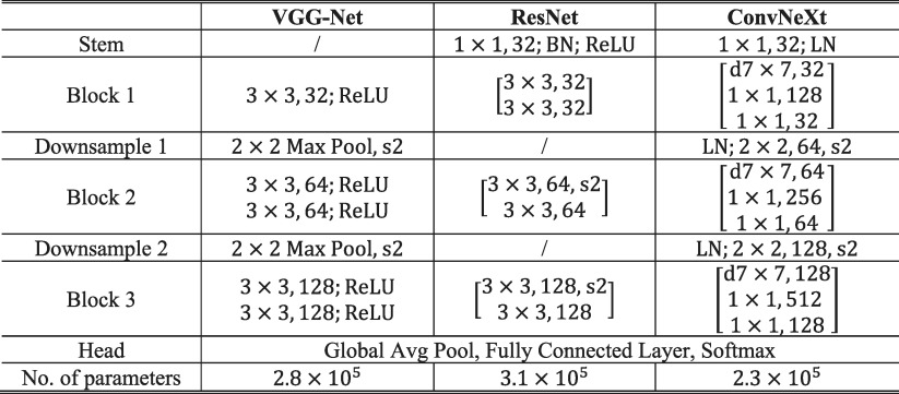
There are variations in the CNN-MC observer modeling. DCNN classifiers with different network structures learn image features differently. Even for the same network structure, the randomness in DCNN training such as kernel initialization or data batching can lead to different local minima. These are akin to the interobserver and intraobserver variabilities of human observers. To account for these variations, we investigated the VGG-Net (Simonyan and Zisserman 2015), the ResNet (He et al 2016) and the ConvNeXt (Liu et al 2022) of similar sizes, as shown in table 1, as the backbone structures of CNN-MC. We also repeated the training multiple times with different random initialization for each structure. The image condition rankings from the individual models and the final combined rankings were analyzed.

Table 1.

Network structures of CNN-MC and CNN-NE in this study.

* The input to the models is a 128 × 128 pixel image patch. BN: batch normalization. LN: layer normalization. Convolutional layers are specified by the kernel size and number of filters. ‘d’ denotes the depth-wise convolution. ‘s2’ denotes the stride-2 operation. The brackets denote ResNet block or ConvNeXt block.

2.2.2. CNN noise estimator (CNN-NE)

It is important to assess the image noise for an image processing technique because enhancing the signals is always associated with a change in noise. We developed a DCNN noise estimator (CNN-NE) to quantify the root-mean-square (RMS) noise level of its input image patch. We designed their network structures to be the same as those for CNN-MC (table 1), except for without the exit softmax function, to facilitate transfer learning (discussed next). The training set contained DBT image patches of breast structured background with the training labels calculated by an ROI-based method for each patch as follows: the patch was divided into 10 × 10 pixel ROIs with 25 pixel spacing on a grid, the ROI background trend was removed by a quadratic fitting, the RMS variations of the ROI pixel values were then calculated and averaged over all ROIs as the RMS noise. The CNN-NE was implemented as a regression model. The training loss was the MSE loss between the estimated RMS noise and the training labels. After training, the CNN-NE model was applied to the test set patches. The average of the estimated RMS noise over all patches was used as a noise measure of the entire set.

2.2.3. Transfer learning

For training CNN-NE and CNN-MC, we adopted the training technique of transfer learning (Yosinski et al 2014, Samala et al 2019). The CNN-NE required only breast structured background images with a range of noise levels so that a large training set could be obtained relatively easily. The trained CNN-NE then served as the pre-trained model to be further fine-tuned as CNN-MC by transfer learning. Since the availability of MC-positive samples was limited, transfer learning reduced the training sample size required and improved the model robustness. It also reused the weights that the model learned from the source task of noise estimation to encourage the CNN-MC to focus on the background noise patterns in the downstream task of MC detection.

2.3. Data sets

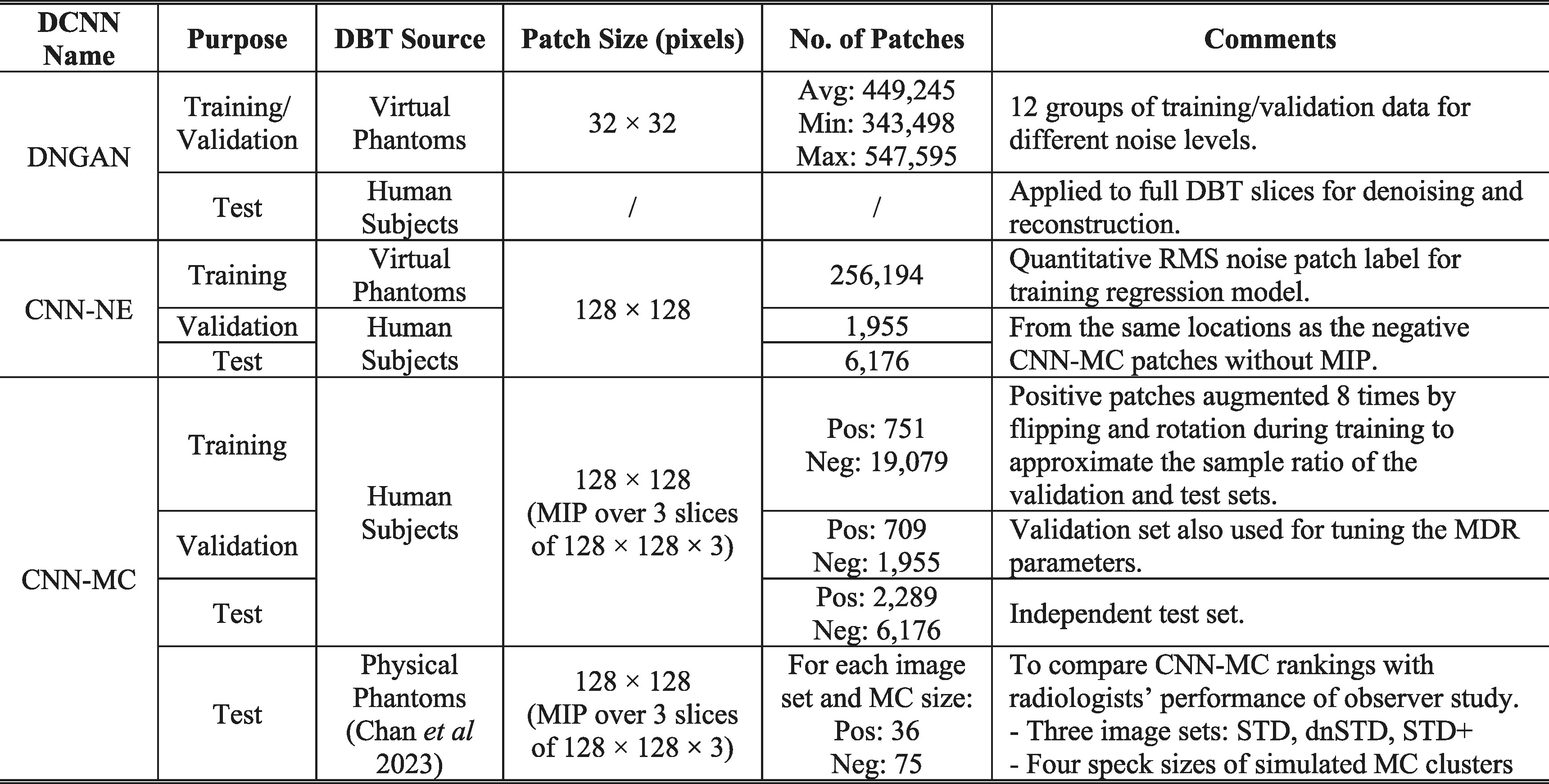
We modeled three DCNNs: DNGAN, CNN-NE and CNN-MC, for denoising, noise estimation, and MC classification, respectively, in this work. To facilitate the training, validation, and testing of these DCNNs, we prepared two primary DBT sources: virtual phantom DBTs and human subject DBTs. This section first provides an overview of these data sources and how they were used for the data sets, as summarized in table 2, and then delves into the details in the following subsections.

Table 2.

Summary of data sets for DCNNs.

* Pixel size of all patches is 0.1 mm × 0.1 mm.

Gao et al (2021a) performed training and validation of DNGAN using virtual phantom DBTs and demonstrated its transferability to human subject DBTs. In the current work, we used the virtual phantom DBTs for the DNGAN training set. This choice was motivated by their flexibility and controllability in generating a wide range of image noise levels with different breast densities and thicknesses. Similar to Gao et al (2021a), we chose a small training patch size of 32 × 32 pixels for DNGAN, allowing it to concentrate on local image structures during adversarial training (Isola et al 2017). The denoiser was fully convolutional at deployment so that the training patch size would not affect the image sizes for which it could be used.

The training set, validation set and independent test set of CNN-MC were prepared using human subject DBTs because we were interested in evaluating the detectability of MC clusters in real patient data and it is difficult to simulate the wide variations in features of real MC clusters by virtual phantom software. The input patch size of CNN-MC was 128 × 128 pixels. This patch size was chosen to cover typical MC clusters in patient cases while keeping the processing time modest.

The CNN-NE training set was extracted from the virtual phantom DBTs that had a wide noise range, similar to the motivation of the DNGAN training set. For the CNN-NE validation and test sets, we had to use the same human subject DBTs as those for CNN-MC. This enabled us to calculate the RMS noise for each reconstruction, which complemented the AUC metric for MC detectability by CNN-MC. These two CNNs therefore provided the two metrics for the task-based image quality assessment plot, as detailed in the Results section below. The input patch size of CNN-NE was the same as CNN-MC because the two networks shared the same structures for transfer learning.

In addition, Chan et al (2023) conducted an observer study with radiologists using a set of physical phantom DBTs with simulated MC clusters to demonstrate the improvement of MC detection by DNGAN denoising. In the current study, we reused their data set to test the capability of CNN-MC in ranking MC detectability relative to human readers. We calculated the relative rankings of the CNN-MC AUC for the MC clusters in the physical phantom DBTs, and then compared them with the relative performance of radiologists’ reading under the image conditions of the observer study.

2.3.1. Virtual phantom DBTs

We generated a collection of virtual breast phantoms at a voxel resolution of 0.05 mm using the anthropomorphic breast model from the Virtual Imaging Clinical Trial for Regulatory Evaluation (VICTRE) package (Badano et al 2018). The VICTRE project considered four breast density categories and one compressed thickness for each category. They stated that this design mirrored the cohort demographics of their comparative clinical trial. In our study, we used the same breast density setting as VICTRE, and slightly varied the thicknesses to make it more varied like human data. In particular, a total of 70 phantoms were simulated at a range of glandular volume fractions (GVF), including 10 almost entirely fatty (5% GVF), 10 scattered fibroglandular dense (15% GVF), 25 heterogeneously dense (34% GVF), and 25 extremely dense (60% GVF). The thicknesses of the compressed phantoms for the four density categories were 52–70 mm at every 2 mm, 46–64 mm at every 2 mm, 36–60 mm at every 1 mm, and 31–55 mm at every 1 mm, respectively.

We generated the PVs using the Monte Carlo x-ray imaging simulator (Badal et al 2021). We configured the scan geometry as 9 PVs in 25° scan angle and 3.125° increments and the x-ray spectrum as 34 kVp Rh/Ag to model the Pristina DBT system (GE Healthcare, Waukesha, WI). The distances between source and isocenter, isocenter and breast support, breast support and detector were 617 mm, 20 mm, 23 mm, respectively. Scatter and electronic noise were not simulated. The exposure was adjusted for each phantom so that the estimated mean glandular dose matched the measured value for that breast thickness from the automatic exposure control (AEC) of Pristina. To simulate a wide range of noise levels, we repeated the simulations and varied the exposure by factors of 0.25, 0.3, 0.35, 0.4, 0.5, 0.6, 0.75, 1, 1.4, 2, 3. These exposure factors were selected such that the noise standard deviations of the post-log x-ray intensity on the PVs, and hence the reconstructed DBT images, were evenly spaced. Finally, we reconstructed the DBT images using 3 iterations of the simultaneous algebraic reconstruction technique (SART) (Zhang et al 2006).

2.3.2. DNGAN training set

For DNGAN training, we used the virtual phantom DBTs with an exposure factor of 3 as the training high dose (HD) targets and the DBTs with the remaining 10 exposure levels as the training low dose (LD) inputs. To ensure that DNGAN covered a wide range of DBT noise levels due to variations in patient sizes and other factors in clinical settings, we trained a suite of DNGAN denoisers, each of which can handle a certain range of image noise levels. To do so, we calculated the average RMS noise for each DBT volume using the method described in section 2.2.2 and obtained the range of the noise values for the entire set of virtual DBT volumes. We empirically grouped the volumes into 12 groups so that the noise interval of each group was reasonably small. We then extracted training patches within the breast regions from each group. This resulted in 12 groups of DNGAN training data with an average of 449 245 (min: 343 498; max: 547 595) LD/HD pairs of 32 × 32 pixel training patches for training a denoiser for each group.

2.3.3. CNN-NE training set

We randomly extracted 128 × 128 pixel patches within the breast regions from all the 70 virtual phantom DBTs and 11 exposure levels to form the CNN-NE training set. This gave a total of 256 194 patches. The low-frequency background was removed from the patches to reduce the nonuniformity caused by heterogeneous breast structures (Chan et al 1995).

2.3.4. Human subject DBTs

We had 238 human subject cases with biopsy-proven MCs collected with Institutional Review Board approval and written informed consent. Two-viewed DBTs of the breast with MCs were acquired for each case using the GEN2 prototype DBT system (GE Global Research, Niskayuna, NY). The system acquired 21 PVs in 60° scan angle and 3° increments with a 29 kVp Rh/Rh x-ray beam. The distances between source and isocenter and between isocenter and detector were 640 mm and 20 mm, respectively. The breast support was at the same height as the isocenter. For our reconstructions, we used the central 9 PVs in 24° angle so that the scan geometry was similar to that of the GE commercial Pristina DBT system. The radiation doses at 9 PVs were similar to those of the Pristina system. A Mammography Quality Standards Act (MQSA) approved radiologist marked the biopsied MCs with 3D bounding boxes in the reconstructed DBT images based on all available clinical information.

2.3.5. CNN-MC training set and CNN-NE/CNN-MC validation and test set

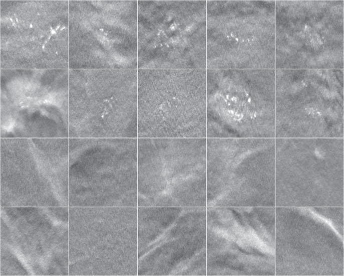
We split the human subject DBTs by case into three disjoint sets for training, validation and testing. The training set consisted of 64 cases, or 127 DBT views (one view was lost due to technical issue). The validation set consisted of 52 cases, or 104 DBT views. The remaining 122 cases with 246 views (one case had bilateral MCs) were sequestered as independent test set. For each data set, positive patches of size 128 × 128 × 3 pixels containing clustered MCs were extracted inside the radiologist’s 3D boxes on a regular grid with centers separated by 128 pixels in the two directions along a slice and separated by 1 slice with offset centers along the depth direction. An MC cluster therefore might be extracted multiple times in part or in whole but spatially shifted in each patch, which served as augmented samples to reduce the imbalance between the two classes. Non-overlapping negative patches of the same size were randomly extracted outside the 3D boxes in the structured breast background. For the CNN-MC, we obtained 751 positive and 19 079 negative patches for the training set, 709 positive and 1955 negative patches for the validation set, and 2289 positive and 6176 negative patches for the test set. For each patch, we removed the low-frequency background and took maximum intensity projection (MIP) over the three slices to emphasize the MCs, if any. Figure 1 shows example MIP patches from the CNN-MC training set. For the validation and test sets of CNN-NE, the same sets of negative patches for CNN-MC were extracted except that only the central slices without MIP were used.

Figure 1.

Example 3-slice MIP patches with MCs (top two rows) and without MCs (bottom two rows) from the CNN-MC training set of human subject DBTs. The patch size is 128 × 128 pixels (12.8 mm × 12.8 mm).

2.3.6. Physical phantom DBTs

The physical phantom DBTs were used in a previous observer study with radiologists to detect MC clusters under three image conditions (Chan et al 2023). Each of the six breast phantoms were 5 cm thick and made of 50% glandular/50% adipose heterogeneous breast-tissue-equivalent materials. Clusters of simulated MCs of four nominal speck diameters (0.125–0.150 mm, 0.150–0.180 mm, 0.180–0.212 mm, 0.212–0.250 mm) were embedded in the phantoms. There were 36 clusters for each diameter range, giving a total of 144 clusters. The phantoms were imaged twice using two automatic exposure modes of the Pristina DBT system: the standard (STD) mode, which was for routine patient imaging, and the STD+ mode, which used about 54% more dose than that of STD. The DBT images were reconstructed by the built-in commercial algorithm. A third image set called dnSTD was obtained by denoising the STD set using the DNGAN denoiser. The denoiser was trained and validated by Gao et al (2021a) using a separate set of physical phantoms that shared the same materials but had different designs from the test phantoms in the Chan et al (2023) study. For each image set and each MC speck size, we extracted a total of 36 128 × 128 pixel background-corrected 3-slice MIP patches centered at the MC clusters as positives and paired them with 75 MC-free background MIP patches as negatives for CNN-MC testing. The set of 75 negative patches was extracted from different random locations for each MC positive set.

2.4. Implementation

For MDR, the implementation of $L_{\text{DBCN}}\left(x\right)$ and $R_{\text{EP}}\left(x\right)$ was described in Zheng et al (2018). The 12 DNGAN denoisers were trained separately following the process described in Gao et al (2021a). We retrained DNGAN using our newly generated training set that had a wider range of noise levels and breast characteristics while keeping all training settings unchanged. When DNGAN was called during reconstruction, the algorithm automatically estimated the RMS noise of the DBT volume at that iteration and selected the denoiser with the closest-matched noise from the 12 trained denoisers for deployment. We chose $N_{\text{iter}}$ and $N_{\text{inner}}$ to 3 experimentally. Section 3.2 discusses the selections of ${\beta }_{\text{EP}}$ and ${\beta }_{\text{RED}}.$ Both $x$ and $z$ were initialized to 0. The image variable $z$ was saved as the final reconstructed image. All the PVs had a pixel size of 0.1 mm × 0.1 mm. The reconstructed images had a voxel size of 0.1 mm × 0.1 mm × 1 mm and were saved in DICOM format with a pixel value range of $\left[0,4095\right].$ Metal artifact reduction (Lu et al 2017) and truncated projection artifact reduction (Lu et al 2013) were implemented to minimize these artifacts in the reconstructed DBT volumes.

For the CNN-NE (CNN-MC) training, we set the number of epochs to 600 (300) and the mini-batch size to 2048 (512). The Adam optimizer was set with an initial learning rate of ${10}^{-3}$ (${10}^{-5}$) and dropped by a factor of 0.8 for every 20 (10) epochs. We initialized the kernel weights of CNN-NE randomly and initialized CNN-MC with the trained CNN-NE. In CNN-MC training, the positive patches were augmented by a factor of 8 (4 rotations by 90 degrees and another 4 rotations after flipping). During CNN-MC deployment, we augmented every patch and averaged the 8 output scores as the patch score. We further averaged the patch scores of all positive patches from the same MC cluster by DBT view for the ROC analysis. We repeated the training of CNN-NE and fine-tuning of CNN-MC 5 times. Each repeated experiment used a different random seed for the weight initialization of CNN-NE and the data batching during CNN-NE training and CNN-MC fine-tuning. We reported the mean and standard deviation of the 5 CNN-MC AUCs. We reported only the mean of the 5 CNN-NE RMS estimates because all standard deviations were smaller than 2% of one pixel value.

2.5. Image conditions

We compared MDR with other approaches, including SART (Zhang et al 2006), SART with multiscale bilateral filtering (MSBF) regularization (Lu et al 2015), DBCN reconstruction (Zheng et al 2018), RED reconstruction without DBCN modeling, and post-reconstruction DNGAN denoising on SART and DBCN images. Gao et al (2023) evaluated DNGAN denoising of PVs for SART reconstruction and observed that it suffered from blurry MCs. Therefore, PV denoising was not considered in this study.

3. Results

3.1. Effectiveness of DNGAN, CNN-NE and CNN-MC

As an example, we deployed one of the five CNN-NE models with VGG-Net backbone trained with different random initializations to the CNN-NE validation set from 2 iterations of SART images. Figure 2 shows that the CNN-NE RMS noise of the individual patches correlated well with the analytical calculations (correlation coefficient = 0.993, p < 0.0001), indicating that CNN-NE can accurately estimate the RMS noise of an input patch. Similar correlations were observed for other reconstructions (not shown). While CNN-NE was trained using VICTRE images from 3 iterations of SART, it was applicable to other reconstructions and human subject images at deployment because it was designed to assess the RMS variations in noisy pixels without relying on the specific image conditions.

Figure 2.

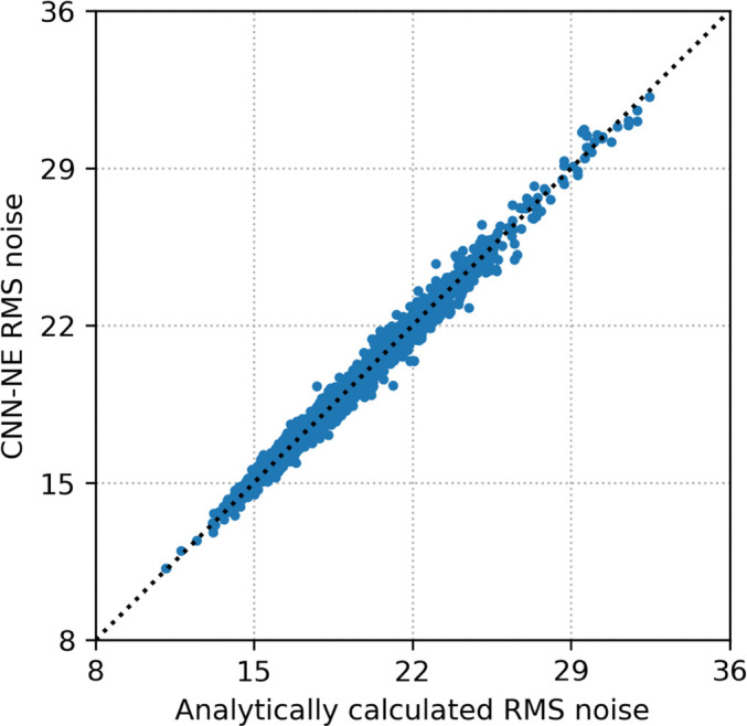
The scatter plot of the CNN-NE estimated RMS noise versus the analytically calculated RMS noise for the individual patches in the CNN-NE validation set (human subject DBT images). The dotted line is the diagonal line. The RMS noise is plotted in terms of pixel values.

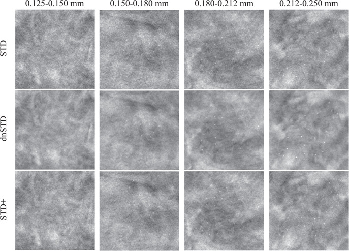
Chan et al (2023) conducted an observer study using physical phantom DBTs and had seven radiologists detect the MC clusters in the STD, dnSTD, and STD+ conditions. Figure 3 shows example of the MC clusters. The study found that the average sensitivities of detecting MC clusters in dnSTD, obtained from DNGAN denoising of the STD images, were higher than those in STD for all 4 MC speck sizes and were comparable to those in STD+. This shows the effectiveness of the DNGAN denoiser to reduce noise and enhance MCs in DBT.

Figure 3.

Example images (18 mm × 18 mm) with MC clusters from the physical phantom DBTs acquired and reconstructed by a GE Pristina DBT system. The dnSTD images were obtained by DNGAN denoising on the STD images. The STD+ mode used 54% more dose than the STD mode.

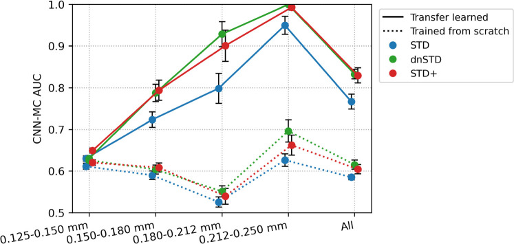
To demonstrate the potential of using CNN-MC in estimating the relative detectability of MC clusters, we applied the CNN-MC models to the extracted patches from the phantom DBTs used in the observer study. The CNN-MC models used VGG-Net backbone and were trained for 2 iterations of SART images. The solid lines in figure 4 show that the AUCs increased with MC speck size. The AUCs of dnSTD were higher than STD and close to STD+. The relative rankings for the speck sizes and the image conditions given by the CNN-MC were consistent with the findings of the observer study. To show the benefit of transfer learning, we repeated the experiment but trained the CNN-MC models from scratch instead of from the pre-trained CNN-NE. In this case, the CNN-MC failed to learn and likely estimated the patch scores based on image features unrelated to MC detectability. This led to very low AUCs and a lack of correlation between MC size and AUC, as shown by the dotted lines in figure 4.

Figure 4.

AUCs of CNN-MC for the classification of image patches with and without MC clusters in the physical phantom DBTs of 3 image conditions. The data points and error bars were obtained from the mean and standard deviation of the 5 repeated models trained with different random initialization. The points are slightly shifted horizontally to avoid overlap.

3.2. Parameter selection for MDR regularization

To select the regularization parameters ${\beta }_{\text{EP}}$ and ${\beta }_{\text{RED}}$ in MDR, we performed a grid search with ${\beta }_{\text{EP}}$ = 30, 50, 70, 90 and ${\beta }_{\text{RED}}$ = 100, 500, 1000, 5000. Figure 5 shows the task-based image quality assessment plot of CNN-MC AUC versus CNN-NE RMS noise for the VGG-Net backbone on the validation set for the different parameters. At a low ${\beta }_{\text{EP}}$ value of 30, the AUCs were low because the noise was poorly suppressed and thus obscured MC conspicuity. As ${\beta }_{\text{EP}}$ increased to 50, the MC signals were enhanced relative to noise and the AUCs were improved. But if ${\beta }_{\text{EP}}$ further increased to 70 or 90, the regularization became so strong that the true MCs were smoothed, resulting in lower AUCs. For a given ${\beta }_{\text{EP}},$ decreasing ${\beta }_{\text{RED}}$ meant a weaker regularization, resulting in higher image noise. On the other hand, reduced regularization placed greater emphasis on the data-fit term, thus enhancing the MC signals. This explains why we observed slight increase in AUC as ${\beta }_{\text{RED}}$ decreased. We selected ${\beta }_{\text{RED}}$ = 500 to balance the tradeoff between noise reduction and signal enhancement. In other parts of this study, we set the regularization parameter ${\beta }_{\text{EP}}$ to 50 and ${\beta }_{\text{RED}}$ to 500 if not specified.

Figure 5.

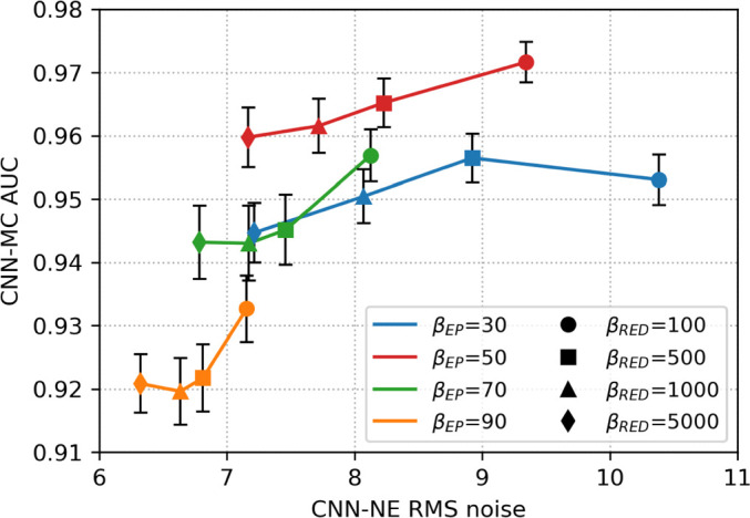
The task-based image quality assessment plot showing the tradeoff between MC cluster detectability (CNN-MC AUC) versus image noise (CNN-NE RMS noise) on the validation set reconstructed with different regularization parameters ${\beta }_{\text{EP}}$ and ${\beta }_{\text{RED}}$ in MDR. The data points obtained with a fixed ${\beta }_{\text{EP}}$ are linked by a solid line and data points for a fixed ${\beta }_{\text{RED}}$ are shown with the same symbol.

3.3. MDR ablation study

We conducted an ablation study to illustrate the effects of the three terms in the MDR cost function (7). The three terms could be turned on or off separately to create 6 partial models. To turn off $L_{\text{DBCN}}\left(x\right),$ we used the regular data-fit term $L_{\text{regular}}\left(x\right)=\frac{1}{2}{\sum }_{i=1}^{N_p}{‖y_i-A_{i}x‖}_2^2$ instead of (4). $R_{\text{EP}}\left(x\right)$ was turned off by setting ${\beta }_{\text{EP}}$ to 0. $R_{\text{RED}}\left(x\right)$ was turned off by setting ${\beta }_{\text{RED}}$ to 0 and skipping all DNGAN denoising.

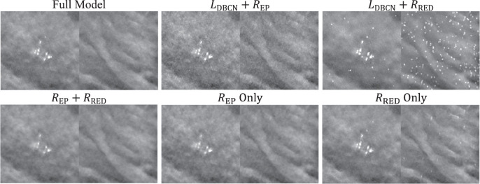
Figure 6 shows the task-based image quality assessment plot for the VGG-Net backbone on the validation set for the different partial MDR models in comparison to the full MDR model. Figure 7 shows examples of MIP patches with and without MCs from the human subject validation set. From ‘$R_{\text{EP}}$ Only’, we found that the EP regularizer (${\beta }_{\text{EP}}$ = 50) encouraged the smoothness of the images but sacrificed the sharpness of the MCs. The $L_{\text{DBCN}}$ term contributed to signal enhancement, as can be seen from the AUC improvement between ‘$R_{\text{EP}}$ Only’ and ‘$L_{\text{DBCN}}+R_{\text{EP}}$’, although it produced exceptionally noisy images if used alone. The ‘$L_{\text{DBCN}}$ Only’ condition (RMS noise: 101.1, AUC: 0.846 ± 0.004) is outside the plot range of figure 6 and is not shown in figure 7. The ‘$L_{\text{DBCN}}+R_{\text{EP}}$’ condition had a high AUC but also a high RMS noise. From ‘$R_{\text{RED}}$ Only’, we observed that the RED regularizer (${\beta }_{\text{RED}}$ = 500) powered by DNGAN was good at noise reduction and signal preservation, but sometimes it falsely enhanced the background tissue structures. Those MC-like enhancements were detected as false positives by CNN-MC and led to an overall low AUC. The false enhancement was even more severe for ‘$L_{\text{DBCN}}+R_{\text{RED}}$’ which had the lowest AUC in figure 6. With ‘$R_{\text{EP}}+R_{\text{RED}}$’, the false positives in the ‘$R_{\text{RED}}$ Only’ condition were suppressed and the RMS noise was the lowest, but it overly smoothed the MCs. Finally, the full MDR model took advantage of all three terms and achieved reasonably low RMS noise and the highest AUC.

Figure 6.

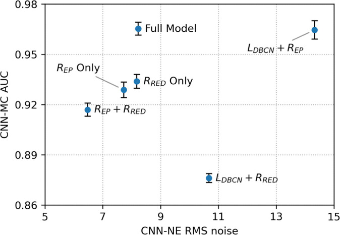
The task-based image quality assessment plot on the validation set showing the tradeoffs of the different terms in the MDR ablation study.

Figure 7.

Example 3-slice MIP patches (12.8 mm × 12.8 mm) from the human subject validation set for the MDR ablation study. In each pair, a positive patch of MC cluster is shown on the left and a negative MC-free patch on the right.

3.4. Comparisons on validation set and independent test set

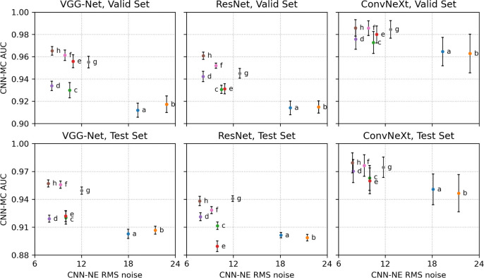
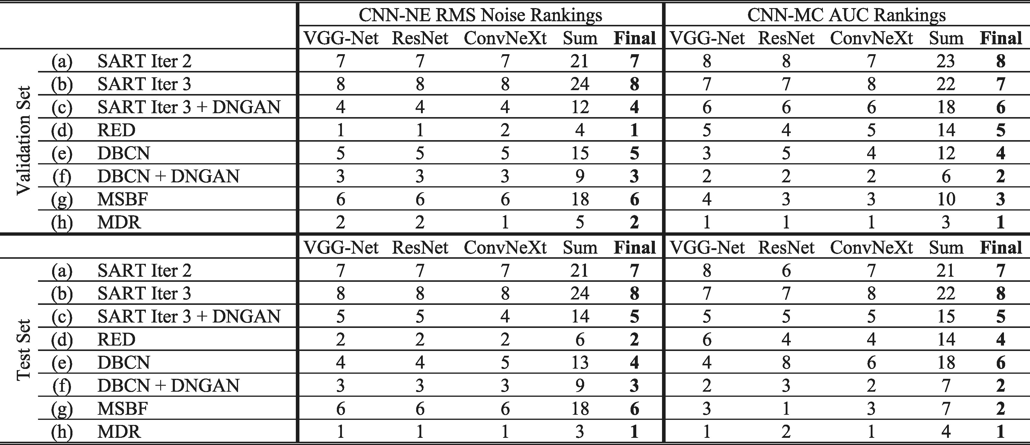
We compared eight image conditions in this section: (a) SART iteration 2; (b) SART iteration 3; (c) SART iteration 3 with post-reconstruction DNGAN denoising; (d) RED without DBCN modeling, equivalent to ‘$R_{\text{RED}}$ Only’ in section 3.3; (e) DBCN ($\beta$ = 70); (f) DBCN ($\beta$ = 50) with post-reconstruction DNGAN denoising; (g) MSBF; (h) MDR. Figure 8 shows the task-based image quality assessment plot for the validation set and the independent test set using the VGG-Net, ResNet and ConvNeXt backbones. The VGG-Net and ResNet had smaller error bars for AUCs and thus better reproducibility than ConvNeXt. The AUC and RMS noise rankings given by the three networks had some variations but were mostly consistent within the error bars. Table 3 summarizes the RMS noise and AUC ranking results in figure 8. The final rankings were obtained by summing the individual rankings. The rankings on the validation set largely agreed with those on the independent test set with minor variations between adjacent ranks except for DBCN, indicating reasonable generalizability of the proposed DCNN image quality assessment approach to the unseen test set.

Figure 8.

The task-based image quality assessment plot on the human subject validation set (first row) and test set (second row) using the VGG-Net (left column), ResNet (middle column) and ConvNeXt (right column) for comparing the reconstruction and denoising approaches. The labels (a) to (h) are defined in section 3.4 and table 3.

Table 3.

Summary of rankings for different reconstruction and denoising approaches using DCNN task-based image quality assessment in figure 8.

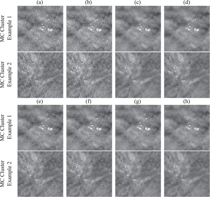
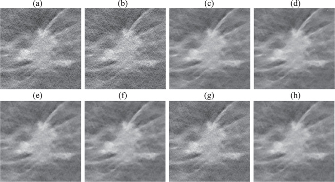
Figure 9 shows the example MIP patches of MC clusters and figure 10 shows example images of a spiculated mass from the human subject test set. The visual judgment of the noise levels matched the quantitative RMS noise estimation. The SART images (conditions (a) and (b)) were noisy with poor MC conspicuity as it is an unregularized reconstruction method (Jiang and Wang 2003). Increasing the number of SART iterations enhanced the signal, but it also amplified noise, resulting in comparable signal-to-noise ratios and thus AUCs, as illustrated in figure 8. This observation reaffirmed our understanding of SART that there was no benefit of continuing SART iterations without regularization. Furthermore, it highlighted the advantage of our task-based metric using CNN-MC, which focused on the detectability of the MC clusters and provided a more informative assessment. DBCN (condition (e)) had relatively large variations of AUC rankings among the three CNN-MCs and two data sets, possibly because its patchy and noisy background confused the image features and made the training set less representative of the data distribution. Post-reconstruction denoising with DNGAN was flexible for application to different reconstruction techniques, reducing image noise and improving the AUC as shown in the examples for both SART (condition (c) in comparison to (b)) and DBCN (condition (f) in comparison to (e)). Note that, with DNGAN denoising, SART and DBCN could use parameters of stronger MC enhancement (3 iterations instead of 2 in SART, and $\beta$ = 50 instead of 70 in DBCN). Although RED (condition (d)) reached a very low noise level and its visual signal quality was comparable to that of MDR, its AUC was low due to false enhancement as discussed in section 3.3. The conspicuous bright spots resembling MCs in the examples shown in figure 7 (lower right) and figure 10(d) reiterated this downside of RED. The AUC ranking of MSBF (condition (g)) was high, but its noise also remained high. The proposed MDR (condition (h)) achieved one of the lowest RMS noise and the highest AUC rankings than other image conditions. The high visibility of the subtle MCs and smooth background of the MDR images can also be clearly seen in figure 9. Moreover, it preserved the fine texture details and had a satisfactory visual quality of mass margins without creating artifact in figure 10.

Figure 9.

Example 3-slice MIP patches (12.8 mm × 12.8 mm) of two MC clusters (example 1: ductal carcinoma in situ; example 2: invasive ductal carcinoma) from the human subject test set. The labels (a) to (h) are defined in section 3.4 and table 3.

Figure 10.

Example images (20 mm × 20 mm) of a spiculated mass (invasive ductal carcinoma) of a human subject DBT. The labels (a) to (h) are defined in section 3.4 and table 3.

3.5. Qualitative comparison between MDR and commercial reconstruction

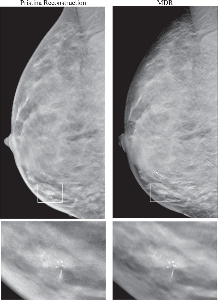
The GEN2 DBT system used for acquiring the human subject DBTs was developed as a prototype for research purposes, so it lacked a built-in reconstruction method. To compare the proposed MDR with gold standard reconstruction, we reconstructed a human subject DBT case acquired with the commercial GE Pristina DBT system. Figure 11 shows a qualitative comparison of the full DBT slices and the zoomed-in views of an MC cluster obtained with the Pristina reconstruction and our MDR approach. The full slice image of MDR had reduced noise levels compared to the Pristina reconstruction. The zoomed images facilitated the visualization of the nuances of the MC signals, surrounding tissue structures, and noise. The MDR not only achieved a substantial reduction in noise, but also preserved details and enhanced the subtle MC specks, demonstrating superior image quality than the commercial reconstruction.

Figure 11.

Qualitative comparison between the commercial GE Pristina reconstruction and the proposed MDR. Top row: full DBT slices (84.4 mm × 170 mm). Bottom row: zoomed-in views of the marked regions (20 mm × 15 mm) containing an MC cluster (ductal carcinoma in situ).

The darkening of breast periphery as seen in the MDR reconstructed image in figure 11 resulted from the physics of x-ray imaging. The reduction in tissue thickness and thus increasing penetration of x-ray exposure to the detector caused varying image intensities near the breast boundaries. Commercial DBT images are generally processed with peripheral equalization software to facilitate radiologists’ reading. We did not attempt to address this issue because we did not have access to any breast peripheral equalization software and its development was outside the scope of this study. One can always view the peripheral regions by adjusting the display contrast and brightness properly. As demonstrated in figure 11, the proposed MDR method enhanced the MC signals regardless of their location. Despite being near the breast periphery, the enlarged ROI still shows the improvement of image quality by the MDR.

4. Discussion

DBCN and DNGAN represent two distinct approaches for enhancing the subtle signals in DBT. The DBCN method approximates the deblurring and noise decorrelation by the inverse of the detector point spread filter and the prewhitening filter. Both operations boost the high frequency signals, which inevitably amplify high frequency noise at the same time. DBCN therefore is incorporated with an EP regularizer to control the noise. DNGAN emphasizes the signals by smoothing the surrounding backgrounds like a regularizer. It also increases the contrast of the signals to some extent, but sometimes falsely enhances the high frequency structures and creates MC-like artifacts. We explored combining the two methods to take advantage of both. We implemented the newly proposed MDR method in an efficient way so that it could reconstruct the full-sized 3D DBT images at full resolution. Quantitative results using our newly developed DCNN image quality measures on the independent test set of human subject DBTs revealed that MDR achieved the highest AUC rankings for MC detectability and low noise among the reconstruction and denoising approaches studied. This study shows the promise of combining the physics-based MBIR and the learning-based DCNNs for reconstruction.

The CNN-MC model observer can characterize the detectability of the MC clusters in human subject DBTs. Because of the complexity of the SKS MC clusters, we trained the CNN-MC to learn the signal representations through back-propagation, unlike CHO and d’ where the target signal is trained to be fitted with channelized functions or mathematically defined. Moreover, the CNN-MC can include the assessment of image background with and without MC-like false enhancement (shown in section 3.3) that the traditional image quality measures such as d’ cannot achieve because they focus on individual signals. Assessing potential false information generated by an image processing method is crucial for evaluating its feasibility in clinical applications.

The role of CNN-NE can be understood from two aspects. First, CNN-NE played a pivotal role in our training and processing pipeline because it served as the pre-trained model of CNN-MC, which worked well only when transfer-learned from CNN-NE (figure 4). The advantages of transfer learning were elaborated in section 2.2.3. Second, despite the possibility of analytically calculating the RMS noise of an image patch, our work showcased the ability of deep CNN to approximate this calculation. There is also a growing interest in applying CNNs for noise quantification in medical imaging (Huber et al 2023). The development of CNN-NE provides users the flexibility of choosing between analytical and CNN calculations for estimating the RMS noise. It is noteworthy that CNN-NE has superior computational efficiency when run on a GPU, compared to the time-consuming grid-based calculation method. We proposed to use CNN-NE and CNN-MC together to guide the selection of the reconstruction parameters and compare different reconstruction techniques and denoising approaches. The task-based image quality assessment plot of CNN-MC AUC versus CNN-NE RMS noise clearly illustrates the tradeoff between the detectability and noise of the different image conditions.

The RMS noise calculation introduced in section 2.2.2 involved a quadratic fitting step to remove the background trend. Given that we used VICTRE simulation data for CNN-NE training and simulations can produce (nearly) noise-free images, it is possible to remove the background structures using such noise-free images. To verify that the RMS noise in images could be effectively estimated by the quadratic fitting background removal method, we simulated the nearly noise-free images using an exposure factor of 10, and then calculated the RMS values for the CNN-NE training image patches with the exposure factor of 1 using the two approaches. The result showed that the two sets of RMS values were close and exhibited a strong linear correlation (correlation coefficient = 0.983, p < 0.0001), indicating the effectiveness of quadratic fitting for background removal. While using noise-free images may be the ideal approach for accurate RMS calculations, its real-world impact is limited due to the linearity and small differences. More importantly, having the noise-free images is a special case and they are typically unavailable for actual scanned images. Therefore, we employed the fitting method in our work due to its practicality in general scenarios in case others would want to adopt the method for their applications.

A suboptimal CNN-MC model observer is preferred for evaluating the effectiveness of image processing techniques since image processing is not expected to improve the performance of an ideal observer. Zhang et al (2021) showed that a DCNN could be trained to approximate an ideal observer or a suboptimal observer, depending on its learning capacity and the available training sample size, for the task of detecting MC clusters in a simulation study. This is consistent with the observations in our study. We found that DCNNs of very deep structures reached an AUC of 1 regardless of the image conditions. We had to constrain the learning capacity by limiting the network sizes such that they could discriminate between the image conditions. In addition, it is known that human observers are suboptimal, as also demonstrated by Chan et al (2023). Since there are no specific guides for selecting the DCNN structure for a given task, we investigated three CNN-MC backbones. The pooled performance of the multiple models may partly alleviate the learning variability, in analogy to the use of multiple observers to account for the interobserver variability in human reader studies. The CNN-NE trained as a regression model was much more stable, as observed from the small variances among the different initializations and different CNN backbones.

We did not analyze the convergence property of MDR in this study. Due to the limited-angle nature of the DBT scan and the fact that radiologists are accustomed to the tissue texture appearance of the 2D projection mammograms, we usually do early stopping on the DBT reconstruction so that the soft tissue structured backgrounds are not overly enhanced. The truncation artifact correction (Lu et al 2013) during reconstruction essentially changes the system matrices and also complicates the convergence analysis. Furthermore, the RED assumptions are not satisfied by many popular denoisers including DNGAN (Reehorst and Schniter 2019). Without the explicit expression and minimization of a cost function, RED serves only as a motivation and one can at best hope to obtain the fixed-point convergence or an equilibrium of the reconstruction (Buzzard et al 2018, Ryu et al 2019). For these reasons, we focused on image quality instead of seeking the convergence of the iterates.

There are limitations in the current study. First, the DNGAN denoisers were trained on the SART images but were directly applied to the intermediate images of MDR. This introduced a noise mismatch between the denoiser and the images to be denoised. The fact that the DNGAN works well in MDR indicates the flexibility of the application, but it also leaves room for improvement by fine-tuning the DNGAN denoisers at every MDR iteration, which will tradeoff computational efficiency, however. Second, the number of MC clusters in our data set is limited. A larger CNN-MC training set may further improve the generalizability of the CNN-MC model observer and reduce the AUC variations among the different DCNN models or between training and deployment to unseen cases. Third, although MDR achieved the highest MC detectability ranking and low noise, post DBCN reconstruction with DNGAN denoising was also among the top three rankings. Post-reconstruction denoising is the only practical approach if the raw PVs are not available for user-designed reconstruction. It will be of interest to evaluate the effectiveness of DNGAN denoising for the DBT images reconstructed by the various commercial DBT systems when large human subject data sets with subtle MCs from these systems become available. Fourth, the proposed DCNN image evaluation approach only focused on image noise and MC detectability. The evaluations of mass and tissue textures still relied on visual judgment. It will be useful if DCNN models can be developed to assess the quality of these important image features as well in the future. Finally, we do not address the time efficiency of MBIR as it falls outside the primary scope of this paper. We encourage future research to tackle this issue, which may complement and enhance the utility of the proposed method.

5. Conclusion

We proposed MDR by combining DBCN modeling and DNGAN denoising using the RED framework for DBT reconstruction. To facilitate the task-based image quality assessment, we also proposed two DCNN tools. The CNN-NE was trained to estimate the RMS noise of the DBT images. The CNN-MC was trained to be a model observer to evaluate the detectability of clustered MCs. The efficacies of DNGAN, CNN-NE and CNN-MC were demonstrated using physical phantom DBTs and human subject DBTs. We investigated the impacts of the MDR regularization parameters and the cost function terms. MDR reduced image noise and improved MC detectability on an independent test set of human subject DBTs. The proposed CNN-NE and CNN-MC evaluation method can serve as a surrogate for human observers to provide task-specific metrics and rank the imaging systems in a cost-effective way. The proposed reconstruction method may potentially lead to lower dose and higher sensitivity and specificity for MC detection in breast cancer screening and diagnosis.

Data availability statement

The data cannot be made publicly available upon publication because the cost of preparing, depositing and hosting the data would be prohibitive within the terms of this research project. The data that support the findings of this study are available upon reasonable request from the authors.

References

- Aggarwal H K, Mani M P, Jacob M. MoDL: model-based deep learning architecture for inverse problems. IEEE Trans. Med. Imaging. 2019;38:394–405. doi: 10.1109/TMI.2018.2865356. [DOI] [PMC free article] [PubMed] [Google Scholar]
- Ahmad R, Bouman C A, Buzzard G T, Chan S, Liu S, Reehorst E T, Schniter P. Plug-and-play methods for magnetic resonance imaging: using denoisers for image recovery. IEEE Signal Process Mag. 2020;37:105–16. doi: 10.1109/MSP.2019.2949470. [DOI] [PMC free article] [PubMed] [Google Scholar]
- Badal A, Cha K H, Divel S, Graff C G, Zeng R, Badano A. Virtual clinical trial for task-based evaluation of a deep learning synthetic mammography algorithm. Proc. SPIE. 2019;2019:109480O. doi: 10.1117/12.2513062. [DOI] [Google Scholar]
- Badal A, Sharma D, Graff C G, Zeng R, Badano A. Mammography and breast tomosynthesis simulator for virtual clinical trials. Comput. Phys. Commun. 2021;261:107779. doi: 10.1016/j.cpc.2020.107779. [DOI] [Google Scholar]
- Badano A, Graff C G, Badal A, Sharma D, Zeng R, Samuelson F W, Glick S J, Myers K J. Evaluation of digital breast tomosynthesis as replacement of full-field digital mammography using an in silico imaging trial. JAMA Netw. Open. 2018;1:e185474. doi: 10.1001/jamanetworkopen.2018.5474. [DOI] [PMC free article] [PubMed] [Google Scholar]
- Balta C, Bouwman R W, Sechopoulos I, Broeders M J M, Karssemeijer N, van Engen R E, Veldkamp W J H. Can a channelized Hotelling observer assess image quality in acquired mammographic images of an anthropomorphic breast phantom including image processing? Med. Phys. 2019;46:714–25. doi: 10.1002/mp.13342. [DOI] [PubMed] [Google Scholar]
- Barrett H H, Yao J, Rolland J P, Myers K J. Model observers for assessment of image quality. Proc. Natl Acad. Sci. 1993;90:9758–65. doi: 10.1073/pnas.90.21.9758. [DOI] [PMC free article] [PubMed] [Google Scholar]
- Buzzard G T, Chan S H, Sreehari S, Bouman C A. Plug-and-play unplugged: optimization-free reconstruction using consensus equilibrium. SIAM J. Imaging Sci. 2018;11:2001–20. doi: 10.1137/17M1122451. [DOI] [Google Scholar]
- Chan H-P, et al. Digital breast tomosynthesis: observer performance of clustered microcalcification detection on breast phantom images acquired with an experimental system using variable scan angles, angular increments, and number of projection views. Radiology. 2014;273:675–85. doi: 10.1148/radiol.14132722. [DOI] [PMC free article] [PubMed] [Google Scholar]
- Chan H-P, et al. Deep learning denoising of digital breast tomosynthesis: observer performance study of the effect on detection of microcalcifications in breast phantom images. Med. Phys. 2023;50:6177–89. doi: 10.1002/mp.16439. [DOI] [PMC free article] [PubMed] [Google Scholar]
- Chan H-P, Wei D, Helvie M A, Sahiner B, Adler D D, Goodsitt M M, Petrick N. Computer-aided classification of mammographic masses and normal tissue: linear discriminant analysis in texture feature space. Phys. Med. Biol. 1995;40:857–76. doi: 10.1088/0031-9155/40/5/010. [DOI] [PubMed] [Google Scholar]
- Chong A, Weinstein S P, McDonald E S, Conant E F. Digital breast tomosynthesis: concepts and clinical practice. Radiology. 2019;292:1–14. doi: 10.1148/radiol.2019180760. [DOI] [PMC free article] [PubMed] [Google Scholar]
- Das M, Gifford H C, O’Connor J M, Glick S J. Penalized maximum likelihood reconstruction for improved microcalcification detection in breast tomosynthesis. IEEE Trans. Med. Imaging. 2011;30:904–14. doi: 10.1109/TMI.2010.2089694. [DOI] [PMC free article] [PubMed] [Google Scholar]
- Gang G J, Lee J, Stayman J W, Tward D J, Zbijewski W, Prince J L, Siewerdsen J H. Analysis of Fourier-domain task-based detectability index in tomosynthesis and cone-beam CT in relation to human observer performance. Med. Phys. 2011;38:1754–68. doi: 10.1118/1.3560428. [DOI] [PMC free article] [PubMed] [Google Scholar]
- Gao M, Fessler J A, Chan H-P. Deep convolutional neural network with adversarial training for denoising digital breast tomosynthesis images. IEEE Trans. Med. Imaging. 2021a;40:1805–16. doi: 10.1109/TMI.2021.3066896. [DOI] [PMC free article] [PubMed] [Google Scholar]
- Gao M, Helvie M A, Samala R K, Hadjiyski L M, Fessler J A, Chan H-P. Deep CNN task-based image quality assessment: application to digital breast tomosynthesis reconstruction and denoising. Proc. SPIE. 2023;2023:1246319. doi: 10.1117/12.2655419. [DOI] [Google Scholar]
- Gao M, Samala R K, Fessler J A, Chan H-P. Deep convolutional neural network denoising for digital breast tomosynthesis reconstruction. Proc. SPIE. 2020;2020:113120Q. doi: 10.1117/12.2549361. [DOI] [Google Scholar]
- Gao Y, Moy L, Heller S L. Digital breast tomosynthesis: update on technology, evidence, and clinical practice. RadioGraphics. 2021b;41:321–37. doi: 10.1148/rg.2021200101. [DOI] [PMC free article] [PubMed] [Google Scholar]
- Gilbert F J, Tucker L, Young K C. Digital breast tomosynthesis (DBT): a review of the evidence for use as a screening tool. Clin. Radiol. 2016;71:141–50. doi: 10.1016/j.crad.2015.11.008. [DOI] [PubMed] [Google Scholar]
- Gomi T, Kijima Y, Kobayashi T, Koibuchi Y. Evaluation of a generative adversarial network to improve image quality and reduce radiation-dose during digital breast tomosynthesis. Diagnostics. 2022;12:495. doi: 10.3390/diagnostics12020495. [DOI] [PMC free article] [PubMed] [Google Scholar]
- Gulrajani I, Ahmed F, Arjovsky M, Dumoulin V, Courville A. Improved training of Wasserstein GANs. Adv. Neural Inf. Process. Syst. 2017;2017:5769–79. [Google Scholar]
- Haneda E, Tkaczyk J E, Palma G, Iordache R, Zelakiewicz S, Muller S, De Man B. Toward a dose reduction strategy using model-based reconstruction with limited-angle tomosynthesis. Proc. SPIE. 2014;2014:90330V. doi: 10.1117/12.2042897. [DOI] [Google Scholar]
- He J, Yang Y, Wang Y, Zeng D, Bian Z, Zhang H, Sun J, Xu Z, Ma J. Optimizing a parameterized plug-and-play ADMM for iterative low-dose CT reconstruction. IEEE Trans. Med. Imaging. 2019;38:371–82. doi: 10.1109/TMI.2018.2865202. [DOI] [PubMed] [Google Scholar]
- He K, Zhang X, Ren S, Sun J. Deep residual learning for image recognition. IEEE Conf. on Computer Vision and Pattern Recognition; 2016. pp. pp 770–8. [DOI] [Google Scholar]
- Hu Y H, Zhao W. The effect of angular dose distribution on the detection of microcalcifications in digital breast tomosynthesis. Med. Phys. 2011;38:2455–66. doi: 10.1118/1.3570580. [DOI] [PMC free article] [PubMed] [Google Scholar]
- Huber N R, Kim J, Leng S, Mccollough C H, Yu L. Deep learning-based image noise quantification framework for computed tomography. J. Comput. Assist. Tomogr. 2023;47:603–7. doi: 10.1097/RCT.0000000000001469. [DOI] [PMC free article] [PubMed] [Google Scholar]
- ICRU Medical imaging: the Assessment of Image Quality 54 . 1996 doi: 10.1093/jicru/os28.1.Report54. [DOI]
- Isola P, Zhu J-Y, Zhou T, Efros A A. Image-to-image translation with conditional adversarial networks. IEEE Conf. on Computer Vision and Pattern Recognition; 2017. pp. pp 5967–76. [DOI] [Google Scholar]
- Jiang M, Wang G. Convergence of the simultaneous algebraic reconstruction technique (SART) IEEE Trans. Image Process. 2003;12:957–61. doi: 10.1109/TIP.2003.815295. [DOI] [PubMed] [Google Scholar]
- Kupinski M A, Edwards D C, Giger M L, Metz C E. Ideal observer approximation using Bayesian classification neural networks. IEEE Trans. Med. Imaging. 2001;20:886–99. doi: 10.1109/42.952727. [DOI] [PubMed] [Google Scholar]
- Lange K, Fessler J A. Globally convergent algorithms for maximum a posteriori transmission tomography. IEEE Trans. Image Process. 1995;4:1430–8. doi: 10.1109/83.465107. [DOI] [PubMed] [Google Scholar]
- Liu Z, Mao H, Wu C-Y, Feichtenhofer C, Darrell T, Xie S. A convnet for the 2020s. IEEE Conf. on Computer Vision and Pattern Recognition; 2022. pp. pp 11966–76. [DOI] [Google Scholar]
- Lu Y, Chan H-P, Wei J, Hadjiiski L M. A diffusion-based truncated projection artifact reduction method for iterative digital breast tomosynthesis reconstruction. Phys. Med. Biol. 2013;58:569–87. doi: 10.1088/0031-9155/58/3/569. [DOI] [PMC free article] [PubMed] [Google Scholar]
- Lu Y, Chan H-P, Wei J, Hadjiiski L M, Samala R K. Multiscale bilateral filtering for improving image quality in digital breast tomosynthesis. Med. Phys. 2015;42:182–95. doi: 10.1118/1.4903283. [DOI] [PMC free article] [PubMed] [Google Scholar]
- Lu Y, Chan H-P, Wei J, Hadjiiski L M, Samala R K. Improving image quality for digital breast tomosynthesis: an automated detection and diffusion-based method for metal artifact reduction. Phys. Med. Biol. 2017;62:7765–83. doi: 10.1088/1361-6560/aa8803. [DOI] [PMC free article] [PubMed] [Google Scholar]
- Michielsen K, Nuyts J, Cockmartin L, Marshall N, Bosmans H. Design of a model observer to evaluate calcification detectability in breast tomosynthesis and application to smoothing prior optimization. Med. Phys. 2016;43:6577–87. doi: 10.1118/1.4967268. [DOI] [PubMed] [Google Scholar]
- Monga V, Li Y, Eldar Y C. Algorithm unrolling: interpretable, efficient deep learning for signal and image processing. IEEE Signal Process Mag. 2021;38:18–44. doi: 10.1109/MSP.2020.3016905. [DOI] [Google Scholar]
- Nuyts J, De Man B, Fessler J A, Zbijewski W, Beekman F J. Modelling the physics in the iterative reconstruction for transmission computed tomography. Phys. Med. Biol. 2013;58:R63–R96. doi: 10.1088/0031-9155/58/12/R63. [DOI] [PMC free article] [PubMed] [Google Scholar]
- Petrov D, Marshall N W, Young K C, Bosmans H. Systematic approach to a channelized Hotelling model observer implementation for a physical phantom containing mass-like lesions: application to digital breast tomosynthesis. Phys. Med. 2019;58:8–20. doi: 10.1016/j.ejmp.2018.12.033. [DOI] [PubMed] [Google Scholar]
- Reehorst E T, Schniter P. Regularization by denoising: clarifications and new interpretations. IEEE Trans. Comput. Imaging. 2019;5:52–67. doi: 10.1109/TCI.2018.2880326. [DOI] [PMC free article] [PubMed] [Google Scholar]
- Romano Y, Elad M, Milanfar P. The little engine that could: regularization by denoising (RED) SIAM J. Imaging Sci. 2017;10:1804–44. doi: 10.1137/16M1102884. [DOI] [Google Scholar]
- Ryu E K, Liu J, Wang S, Chen X, Wang Z, Yin W. Plug-and-play methods provably converge with properly trained denoisers. Int. Conf. on Machine Learning; 2019. [Google Scholar]
- Sahu P, Huang H, Zhao W, Qin H. Using virtual digital breast tomosynthesis for de-noising of low-dose projection images. Int. Symp. on Biomedical Imaging; 2019. pp. pp 1647–51. [DOI] [Google Scholar]
- Samala R K, Chan H-P, Hadjiiski L, Helvie M A, Richter C D, Cha K H. Breast cancer diagnosis in digital breast tomosynthesis: effects of training sample size on multi-stage transfer learning using deep neural nets. IEEE Trans. Med. Imaging. 2019;38:686–96. doi: 10.1109/TMI.2018.2870343. [DOI] [PMC free article] [PubMed] [Google Scholar]
- Shan H, Padole A, Homayounieh F, Kruger U, Khera R D, Nitiwarangkul C, Kalra M K, Wang G. Competitive performance of a modularized deep neural network compared to commercial algorithms for low-dose CT image reconstruction. Nat. Mach. Intell. 2019;1:269–76. doi: 10.1038/s42256-019-0057-9. [DOI] [PMC free article] [PubMed] [Google Scholar]
- Sidky E Y, Pan X, Reiser I S, Nishikawa R M, Moore R H, Kopans D B. Enhanced imaging of microcalcifications in digital breast tomosynthesis through improved image-reconstruction algorithms. Med. Phys. 2009;36:4920–32. doi: 10.1118/1.3232211. [DOI] [PMC free article] [PubMed] [Google Scholar]
- Simonyan K, Zisserman A. Very deep convolutional networks for large-scale image recognition. Int. Conf. on Learning Representations; 2015. [Google Scholar]
- Solomon J B, Samei E. Correlation between human detection accuracy and observer model-based image quality metrics in computed tomography. J. Med. Imaging. 2016;3:035506. doi: 10.1117/1.JMI.3.3.035506. [DOI] [PMC free article] [PubMed] [Google Scholar]
- Su T, Deng X, Yang J, Wang Z, Fang S, Zheng H, Liang D, Ge Y. DIR-DBTnet: deep iterative reconstruction network for three-dimensional digital breast tomosynthesis imaging. Med. Phys. 2021;48:2289–300. doi: 10.1002/mp.14779. [DOI] [PubMed] [Google Scholar]
- Sundell V-M, Jousi M, Hukkinen K, Blanco R, Mäkelä T, Kaasalainen T. A phantom study comparing technical image quality of five breast tomosynthesis systems. Phys. Med. 2019;63:122–30. doi: 10.1016/j.ejmp.2019.06.004. [DOI] [PubMed] [Google Scholar]
- Teuwen J, Moriakov N, Fedon C, Caballo M, Reiser I, Bakic P, García E, Diaz O, Michielsen K, Sechopoulos I. Deep learning reconstruction of digital breast tomosynthesis images for accurate breast density and patient-specific radiation dose estimation. Med. Image Anal. 2021;71:102061. doi: 10.1016/j.media.2021.102061. [DOI] [PubMed] [Google Scholar]
- Venkatakrishnan S V, Bouman C A, Wohlberg B. Plug-and-play priors for model based reconstruction. IEEE Global Conf. on Signal and Information Processing; 2013. pp. pp 945–8. [DOI] [Google Scholar]
- Wang G, Jacob M, Mou X, Shi Y, Eldar Y C. Deep tomographic image reconstruction: yesterday, today, and tomorrow—editorial for the 2nd special issue ‘machine learning for image reconstruction. IEEE Trans. Med. Imaging. 2021;40:2956–64. doi: 10.1109/TMI.2021.3115547. [DOI] [Google Scholar]
- Wang G, Ye J C, De Man B. Deep learning for tomographic image reconstruction. Nat. Mach. Intell. 2020;2:737–48. doi: 10.1038/s42256-020-00273-z. [DOI] [Google Scholar]
- Wolterink J M, Leiner T, Viergever M A, Isgum I. Generative adversarial networks for noise reduction in low-dose CT. IEEE Trans. Med. Imaging. 2017;36:2536–45. doi: 10.1109/TMI.2017.2708987. [DOI] [PubMed] [Google Scholar]
- Wu D, Kim K, Li Q. Digital breast tomosynthesis reconstruction with deep neural network for improved contrast and in-depth resolution. Int. Symp. on Biomedical Imaging; 2020. pp. pp 656–9. 2020. [DOI] [Google Scholar]
- Xie Z, Baikejiang R, Li T, Zhang X, Gong K, Zhang M, Qi W, Asma E, Qi J. Generative adversarial network based regularized image reconstruction for PET. Phys. Med. Biol. 2020;65:125016. doi: 10.1088/1361-6560/ab8f72. [DOI] [PMC free article] [PubMed] [Google Scholar]
- Xu S, Lu J, Zhou O, Chen Y. Statistical iterative reconstruction to improve image quality for digital breast tomosynthesis. Med. Phys. 2015;42:5377–90. doi: 10.1118/1.4928603. [DOI] [PMC free article] [PubMed] [Google Scholar]
- Yang G, et al. DAGAN: deep de-aliasing generative adversarial networks for fast compressed sensing MRI reconstruction. IEEE Trans. Med. Imaging. 2018;37:1310–21. doi: 10.1109/TMI.2017.2785879. [DOI] [PubMed] [Google Scholar]
- Yang Y, Sun J, Li H, Xu Z. Deep ADMM-Net for compressive sensing MRI. Adv. Neural Inf. Process. Syst.; 2016. pp. 10–8. [Google Scholar]
- Ye D H, Srivastava S, Thibault J-B, Sauer K, Bouman C. Deep residual learning for model-based iterative CT reconstruction using plug-and-play framework. IEEE Int. Conf. on Acoustics, Speech and Signal Processing; 2018. pp. pp 6668–72. [DOI] [Google Scholar]
- Yosinski J, Clune J, Bengio Y, Lipson H. How transferable are features in deep neural networks?. Adv. Neural Inf. Process. Syst.; 2014. pp. 3320–8. [Google Scholar]
- Zeng R, Samuelson F W, Sharma D, Badal A, Christian G G, Glick S J, Myers K J, Badano A. Computational reader design and statistical performance evaluation of an in silico imaging clinical trial comparing digital breast tomosynthesis with full-field digital mammography. J. Med. Imaging. 2020;7:042802. doi: 10.1117/1.JMI.7.4.042802. [DOI] [PMC free article] [PubMed] [Google Scholar]
- Zhang X, Kelkar V A, Granstedt J, Li H, Anastasio M A. Impact of deep learning-based image super-resolution on binary signal detection. J. Med. Imaging. 2021;8:065501. doi: 10.1117/1.JMI.8.6.065501. [DOI] [PMC free article] [PubMed] [Google Scholar]
- Zhang Y, Chan H-P, Sahiner B, Wei J, Goodsitt M M, Hadjiiski L M, Ge J, Zhou C. A comparative study of limited-angle cone-beam reconstruction methods for breast tomosynthesis. Med. Phys. 2006;33:3781–95. doi: 10.1118/1.2237543. [DOI] [PMC free article] [PubMed] [Google Scholar]
- Zheng J, Fessler J A, Chan H-P. Detector blur and correlated noise modeling for digital breast tomosynthesis reconstruction. IEEE Trans. Med. Imaging. 2018;37:116–27. doi: 10.1109/TMI.2017.2732824. [DOI] [PMC free article] [PubMed] [Google Scholar]
- Zheng J, Fessler J A, Chan H-P. Effect of source blur on digital breast tomosynthesis reconstruction. Med. Phys. 2019;46:5572–92. doi: 10.1002/mp.13801. [DOI] [PMC free article] [PubMed] [Google Scholar]
Associated Data
This section collects any data citations, data availability statements, or supplementary materials included in this article.